Solar wind rotation rate and shear at coronal hole boundaries
←
→
Page content transcription
If your browser does not render page correctly, please read the page content below
A&A 653, A92 (2021)
https://doi.org/10.1051/0004-6361/202040180                                                                                                               Astronomy
c R. F. Pinto et al. 2021                                                                                                                                  &
                                                                                                                                                          Astrophysics

     Solar wind rotation rate and shear at coronal hole boundaries
                            Possible consequences for magnetic field inversions
   R. F. Pinto1,2 , N. Poirier2 , A. P. Rouillard2 , A. Kouloumvakos2 , L. Griton2 , N. Fargette2 , R. Kieokaew2 ,
                                          B. Lavraud2,3 , and A. S. Brun1

      1
          Département d’Astrophysique/AIM, CEA/IRFU, CNRS/INSU, Univ. Paris-Saclay & Univ. de Paris, 91191 Gif-sur-Yvette, France
      2
          IRAP, Université de Toulouse; UPS-OMP, CNRS, 9 Av. colonel Roche, BP 44346, 31028 Toulouse cedex 4, France
          e-mail: rui.pinto@irap.omp.eu
      3
          Laboratoire d’Astrophysique de Bordeaux, Univ. Bordeaux, CNRS, B18N, Allée Geoffroy Saint-Hilaire, 33615 Pessac, France

      Received 20 December 2020 / Accepted 15 April 2021

                                                                                     ABSTRACT

      Context. In situ measurements by several spacecraft have revealed that the solar wind is frequently perturbed by transient structures
      that have been interpreted as magnetic folds, jets, waves, and flux ropes that propagate rapidly away from the Sun over a large range
      of heliocentric distances. Parker Solar Probe (PSP), in particular, has detected very frequent rotations of the magnetic field vector at
      small heliocentric radial distances, accompanied by surprisingly large solar wind rotation rates. The physical origin of such magnetic
      field bends and switchbacks, the conditions for their survival across the interplanetary space, and their relation to solar wind rotation
      are yet to be clearly understood.
      Aims. We aim to characterise the global properties of the solar wind flows crossed by PSP, to relate those flows to the rotational state
      of the low solar corona, and to identify regions of the solar surface and corona that are likely to be sources of switchbacks and bends.
      Methods. We traced measured solar wind flows from the spacecraft position down to the surface of the Sun to identify their potential
      source regions, and used a global magneto-hydrodynamic model of the corona and solar wind to analyse the dynamical properties
      of those regions. We identify regions of the solar corona for which solar wind speed and rotational shear are important and long-
      lived that can be favourable to the development of magnetic deflections and to their propagation across extended heights in the
      solar wind.
      Results. We show that coronal rotation is highly structured, and that enhanced flow shear and magnetic field gradients develop near
      the boundaries between coronal holes and streamers, and around and above pseudo-streamers, even when such boundaries are aligned
      with the direction of solar rotation. The exact properties and amplitudes of the shears are a combined effect of the forces exerted by the
      rotation of the corona and of its magnetic topology. A large fraction of the switchbacks identified by PSP map back to these regions,
      both in terms of instantaneous magnetic field connectivity and of the trajectories of wind streams that reach the spacecraft.
      Conclusions. We conclude that these regions of strong shears are likely to leave an imprint on the solar wind over large distances and
      to increase the transverse speed variability in the slow solar wind. The simulations and connectivity analysis suggest they could be a
      source of the switchbacks and spikes observed by PSP.
      Key words. Sun: corona – Sun: rotation – solar wind

1. Introduction                                                                                  to the structure of the solar wind and magnetic field at large
                                                                                                 scales, and to how their interplay generates regions with con-
Measurements made by Parker Solar Probe (PSP; Fox et al.                                         trasting magnetic field directions and flows. Interchange recon-
2016) during its first set of orbits revealed several intriguing                                 nection has been pointed out as a potential candidate mechanism
properties of the solar wind at heliocentric distances that had                                  (Fisk & Kasper 2020), as it links large-scale rotation to magnetic
never been probed before. PSP has shown that strong mag-                                         reconnection. Interchange can occur at a variety of scales in the
netic perturbations in the form of localised magnetic field-                                     solar corona, from polar plumes above small magnetic bipoles
line bends, the most intense of which are termed switchbacks                                     inside coronal holes (Wang & Sheeley 2004; Wang et al. 2012;
(SBs), are omnipresent in the pristine solar wind measured                                       Owens & Forsyth 2013) to streamer–coronal hole boundaries.
near the Sun (Bale et al. 2019). PSP observations have also                                          Sudden reversals of the magnetic field have been observed
shown that the magnitude of the transverse (i.e., rotational)                                    for several decades. Early examples can be spotted in obser-
speeds of the solar wind increases rapidly in the corona with                                    vations from the Helios mission (Behannon & Burlaga 1981).
increasing proximity to the solar surface, up to amplitudes that                                 These reversals have since been studied at various distances
were not expected considering its general radial trend higher                                    from the Sun and related to different photospheric, coronal, or
up in the heliosphere (Kasper et al. 2019). However, our cur-                                    heliospheric phenomena (Kahler et al. 1996; Ballegooijen et al.
rent knowledge of the exact way that the solar rotation propa-                                   1998; Balogh et al. 1999; Yamauchi et al. 2004b,a; Velli et al.
gates into and establishes in the highly magnetised solar corona                                 2011; Neugebauer 2012; Wang & Sheeley 2004; Wang et al.
is insufficient to adequately interpret the rotation state of the                                2012; Owens & Forsyth 2013; Neugebauer & Goldstein 2013;
observed solar wind flows. Physical links between these coin-                                    Matteini et al. 2014; Borovsky 2016; Horbury et al. 2018;
cidental phenomena are yet to be identified, but possibly relate                                 Sterling & Moore 2020). Switchbacks observed by PSP display

                                                                                                                                                                             A92, page 1 of 13

                Open Access article, published by EDP Sciences, under the terms of the Creative Commons Attribution License (https://creativecommons.org/licenses/by/4.0),
                                 which permits unrestricted use, distribution, and reproduction in any medium, provided the original work is properly cited.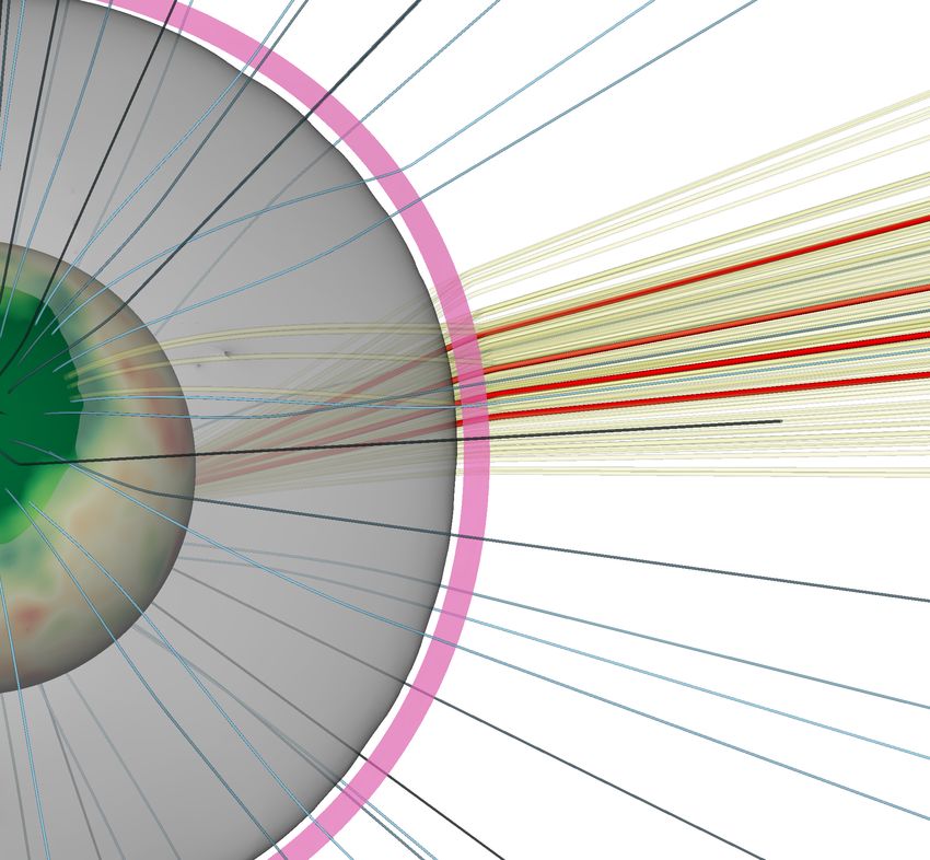
A&A 653, A92 (2021)

a high degree of alfvenicity (cross-helicity), indicating that they    indicate a flatter (more solid-body like) rotation profile, albeit
propagate outwards mostly in the form of incompressible MHD            with substructures that are harder to link to the coronal topology.
waves (Bale et al. 2019), that they correspond to a rotation of             In any case, precisely how the solar rotation establishes
the magnetic field vector without change to its absolute value         throughout the corona, including coronal holes and streamers,
(Mozer et al. 2020), and
                       √ that the transverse velocity (δv⊥ ) and       remains to be fully understood, and whether it can produce sus-
magnetic field (δb⊥ / ρ) perturbations. The physical origin and        tained wind shears is still unknown. Closed magnetic loops will
evolution of magnetic SBs across vast heliocentric distances           tend toward uniform rotation rates all along them (thus opposing
remains elusive. Currently debated hypotheses interpret SBs as         rotation-induced shearing; Grappin et al. 2008), while open field
products of surface and coronal dynamics (reconnection, jets,          lines will develop a wind flow that will see its azimuthal speed
and plumes) or, inversely, claim that they are formed in situ in       decrease with distance from the Sun (in order to conserve angu-
the heliosphere (turbulence, large-scale wind shear). Numerical        lar momentum, as long as the magnetic tension exerted by the
simulations of alfvénic perturbations by Tenerani et al. (2020)        background field becomes weak enough). Streamers are systems
suggest that switchbacks originating in the lower corona may           of closed magnetic loops, and as such should acquire a shape
survive out to PSP distances on their own, but only as long            and rotation pattern that depend on the specific range of solar
as they propagate across a sufficiently unperturbed background         latitudes where they are magnetically rooted. Large streamers
solar wind (free of significant density fluctuations, flow, and        can encompass a large range of magnetic loop sizes and foot-
magnetic shears that could destabilise them; e.g, via the para-        point rotational speeds, and may develop an internal differential
metric instability). However, Owens et al. (2020) argue that solar     rotation structure. Open field lines will follow either a vertical
wind speed shear is an essential factor for the survival of helio-     path or one with strong inflexions around streamers depending
spheric magnetic field inversions (i.e., SBs) produced close to        on where they are rooted at the surface of the Sun, and this
the Sun up to 1 AU, as these should not last long enough without       can have an impact on the transport of angular momentum from
being amplified by solar wind speed shear along their propaga-         the surface up to the high corona. Thus, rotation shearing lay-
tion path. Moreover, Macneil et al. (2020) show that these mag-        ers can develop at specific places on the solar corona, such as at
netic inversions grow in amplitude and in frequency with altitude      the interfaces between coronal holes and streamers. Such shear
in HELIOS data, favouring the idea that they are either created        layers can be of importance to the formation of magnetic field
or amplified by favourable wind shear in the heliophere. From a        reversals, if ever they develop MHD instabilities that allow the
different perspective, Squire et al. (2020) propose that magnetic      transport of mass, vorticy, and helicity across different topolog-
SBs are a natural result of solar wind turbulence, and should          ical regions (via shearing, resistive or Kelvin-Helmhöltz insta-
therefore be produced throughout the heliosphere. Ruffolo et al.       bilities; cf. e.g., Dahlburg & Einaudi 2003; Ruffolo et al. 2020).
(2020) furthermore suggest that shear-driven MHD turbulence            Additionally, the shear patterns formed can be of importance to
is capable of producing magnetic SBs, especially in the regions        the transport and amplification of such magnetic structures (or at
just above the Alfvén surface, where the observed solar wind           least a fraction of them).
flow density transitions from a striated to a flocculated pattern           The first four PSP perihelia occurred during solar minimum,
(cf. DeForest et al. 2016).                                            between about November 2018 and February 2020. During these
     Large-scale solar wind shear builds up naturally from two         close passes, the spacecraft remained within 5 degrees of the
different components: gradients in wind speed in the meridional        solar equator during that time, and also close to the heliospheric
plane (transitions between slow and fast wind streams, between         current sheet (HCS). Solar minimum conditions were charac-
open and closed field regions), and gradients in azimuthal wind        terised by a corona displaying a large equatorial streamer and
speed (rotation). If the role of the former is reasonably easy         two polar coronal holes, essentially in an equator-symmetric
to identify on large scales, that of the latter is much less well      configuration, except for the occurrence of a small low-latitude
understood. The solar photosphere is known to rotate with              CH (visible during the first and second orbits) and a few equa-
a well-defined differential latitudinal profile (with the equa-        torward polar CH extensions and small equatorial CHs.
tor having a higher rotation rate than the poles). The corona               In this paper, we present an investigation of the response of
above, albeit magnetically rooted in the photosphere, seems            the coronal magnetic field and solar wind flows to photospheric
to exhibit a different rotation pattern, with regions that often       rotation, and point out the resulting implications for the interpre-
appear to be rotating rigidly (Antonucci & Svalgaard 1974;             tation of recent measurements made by PSP. We used an MHD
Fisher & Sime 1984). It has been suggested that this rigidity          numerical model of the solar wind and corona, and estimations
could be the result of the interplay between emerging magnetic         of the sun-to-spacecraft connectivity using the IRAP Connectiv-
flux and the global field, involving sustained magnetic recon-         ity Tool to determine the coronal context of the solar wind flows
nection (Wang et al. 1988; Nash et al. 1988). Overall, the coro-       probed by PSP during its first few solar encounters (focusing on
nal plasma seems to rotate with a more solid-body-like pattern         the first, second, and fourth encounters, due to the lack of con-
than the photosphere, particularly at mid and high coronal alti-       tinued good-quality solar wind data for the third encounter). We
tudes (Insley et al. 1995; Bagashvili et al. 2017). The rotation       suggest that the global dynamics of the rotating solar corona can
profile of the corona also seems to evolve over time and to be         impact the conditions for the formation of magnetic disturbances
linked to the solar cycle phase, or at least to the specific coronal   such as SBs (among others).
magnetic field configuration at a given moment (Badalyan et al.
2006; Badalyan 2010). Observations by Giordano & Mancuso
(2008) using SoHO/UVCS show that a number of features super-           2. Numerical model of the rotating corona and wind
pose the average large-scale latitudinal trends of the coronal rota-   2.1. Numerical code and setup
tion during solar minimum. These latter authors observed zones
displaying particularly low rotation rates (or high rotation peri-     We used the numerical code DIP to model a 2.5D axi-symmetric
ods) that are likely to be located near the coronal hole–streamer      solar corona, setup in a similar way to that in Pinto et al. (2016)
boundaries (cf. their Figs. 5 and 6). Similar observations per-        and Pinto et al. (2011), although with a higher spatial resolution
formed during solar maximum (Mancuso & Giordano 2011)                  (768 × 768 grid, non-uniform in radius and uniform in latitude)

A92, page 2 of 13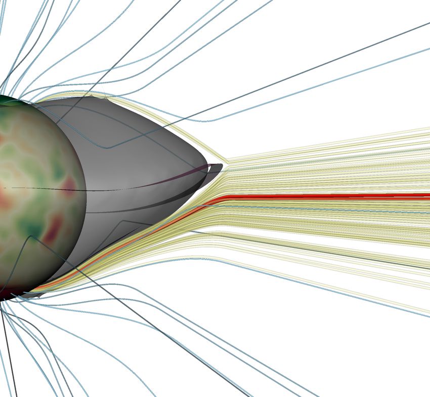
R. F. Pinto et al.: Solar wind speed and rotation shear in the corona

and including rotation. The code solves a system of MHD equa-             little power on the non-alfvén characteristics), accelerating the
tions that describes a one-fluid, isothermal, fully ionised and           open field plasma in the azimuthal direction and exciting a few
compressible plasma:                                                      global oscillations in the closed field regions. After a few Alfvén
                                                                          transit times, and for a small enough , the corona and wind set-
∂t ρ + ∇ · ρu = 0,                                                  (1)   tle down into a quasi-steady state. For  ∼ 1, the highly trans-
       2                                                                  parent surface spins down very quickly, as this configuration
P=        ρkB T,                                                    (2)   corresponds to a lower boundary that cannot oppose the brak-
      mH
                   ∇P J × B                                               ing torque that results from net outward angular momentum flux
∂t u + (u · ∇) u = −   +       − g + ν∇2 u,                         (3)   carried away by the solar wind. For  ∼ 0, the lower coronal
                    ρ     µ0 ρ                                            boundary maintains the imposed rotation, and the magnetic field
∂t B = ∇ × (u × B) + η∇2 B.                                         (4)   is line-tied to it. Smaller closed loops continue to oscillate res-
                                                                          onantly for a long time and the larger ones are sheared indef-
The model assumes the corona and the solar wind to be isother-            initely (as their footpoints suffer a larger range of azimuthal
mal with a uniform coronal temperature T 0 = 1.3 MK and a                 speeds due to differential surface rotation). Intermediate (more
specific heat ratio γ = 1. The magnetic field B separates into            solar-like) values of  allow the surface rotation to be maintained
a time-independent external component B0 (a potential field               in the open-flux regions while the minimal required amount of
resulting from the internal dynamics of the Sun) and into an              footpoint leakage is allowed for the closed-flux regions to sta-
induced field b. We adopted several configurations for B0 in              bilise (cf. Grappin et al. 2008). The streamers gradually evolve
order to simulate different moments of the solar activity cycle.          towards a nearly solid-body rotation profile, with a rotation rate
The equations are integrated using a high-order compact finite            determined by that of the magnetic footpoints. Large stream-
difference scheme (Lele 1992) with third-order Runge-Kutta                ers encompass a wide latitudinal range, and therefore a wide
time-stepping (cf. Grappin et al. 2000). The diffusive terms are          range of footpoint rotation rates. As a result, such streamers
adapted to the local grid scale (∆l), which is non-uniform in             develop a more distinguishable differential rotation pattern than
the radial direction (∆l is minimal close to the lower boundary).         the smaller ones. The open field regions (coronal holes) develop
The kinematic viscosity is defined as ν = ν0 (∆l/∆l0 )2 , typically       permanent azimuthal velocity and magnetic field components,
with ν0 = 2 × 1014 cm2 · s−1 and 0.01 . (∆l/∆l0 )2 . 10. The              with a reasonably complex spatial distribution in the low corona
magnetic diffusivity η is scaled similarly.                               converging into what can be thought of as the beginning of the
     The boundary conditions are formulated in terms of the               Parker spiral on the outer part of the domain. The finite magnetic
MHD characteristics by imposing the amplitudes of the MHD                 resistivity affects the width of these regions, but has a negligi-
characteristics propagating into the numerical domain (the out-           ble effect on the overall rotation rates. We note that in order to
going ones being already completely determined by the dynam-              achieve long-lasting (i.e., stable) coronal rotation profiles we had
ics of the system). The upper boundary is placed at r = 15 R and          to resort to values of  of about 10−3 , rather than to a more realis-
is fully transparent (open to flows and transparent to waves). The        tic  = 10−2 . This is because the convective dynamics of the sur-
lower boundary is placed at r = 1.01 R and is semi-reflective             face and subsurface layers of the Sun are absent from our model,
with respect to the Alfvén mode (but transparent with respect to          and therefore so are the resulting torques that would counter-
all others), and is also open to flows. We treat the chromosphere         balance the weak (but finite) braking torque exerted on the lower
and the transition region layers as an interface (or rather a dis-        boundary by the rotating solar wind.
continuity), and define the chromospheric reflectivity a in terms
of the ratio  of Alfvén wave speeds above and below:
                                                                          2.2. Rotating corona and solar wind: overview
                        photosph
   −1           C
a=     , with  = Acorona ,                                         (5)   We ran a series of numerical MHD simulations of the solar
   +1            CA                                                      corona and wind on which axisymmetric streamers and coronal
                                                                          holes are set under rotation following the methods described in
where C A represents the Alfvén speed B/ (µ0 ρ)1/2 . This approx-         Sect. 2. Figure 1 shows three-dimensional renderings of different
imation is valid for perturbations whose characteristic wave-             simulation runs corresponding to different moments of the solar
length is much greater than the thickness of the chromosphere,            cycle (from left to right: activity minimum, maximum and decay
which is the case for the quasi null-frequency (non-oscillating)          phase) and to different surface rotation profiles (from top to bot-
rotational driver that we apply here at the lower boundary.               tom: differential and solid-body). The blue lines are magnetic
    In order to establish coronal rotation, we first let a non-           field lines. The left halves of the images display meridional cuts
rotating solar wind solution fully develop in the whole numeri-           of the solar wind speed (in units of sonic Mach number, from
cal domain, and then apply a torque at the lower boundary which           0 in solid blue to 2 in solid yellow), while the right side halves
accelerates it progressively to the following rotation rate profile       show the rotation rate Ω (from 0 in black to 14◦ /day in light
Ω (θ) = Ωa + Ωb sin2 θ + Ωc sin4 θ,                                 (6)   orange, defined with respect to the inertial reference frame). The
                                                                          solar surface is coloured with the same colour scheme as the
                                         ◦                      ◦         right side of the images, which serves to illustrate the rotation
with θ being the latitude, Ωa = 14.713 /day, Ωb = −2.396 /day
and Ωc = −1.787◦ /day, following Snodgrass & Ulrich (1990).               pattern at the lower coronal boundary. It is immediately clear
We also tested solid-body solar rotation profiles, which were             from the figure that the solar corona assumes a rotation state
achieved by setting Ωb and Ωc to zero in Eq. (6). The duration of         that is highly structured and that reflects the large-scale topol-
the initial acceleration period was defined to be approximately           ogy of the magnetic field. As described above, the streamers
one-quarter of the average (final) rotation period at the surface,        tend to set themselves into solid body rotation, with the largest
and we let the system relax for at least ten Alfvén crossing times        ones developing a more complex internal rotation structure (with
of the whole domain (lower to upper boundary). The initial tran-          some of its larger inner loops undergoing global resonant trans-
sient propagates upwards (after crossing the idealised chromo-            verse oscillations for a long period of time). Open field lines
spheric interface) predominantly as an Alfvénic wavefront (with           that pass well within coronal holes (far away from CH–streamer

                                                                                                                              A92, page 3 of 13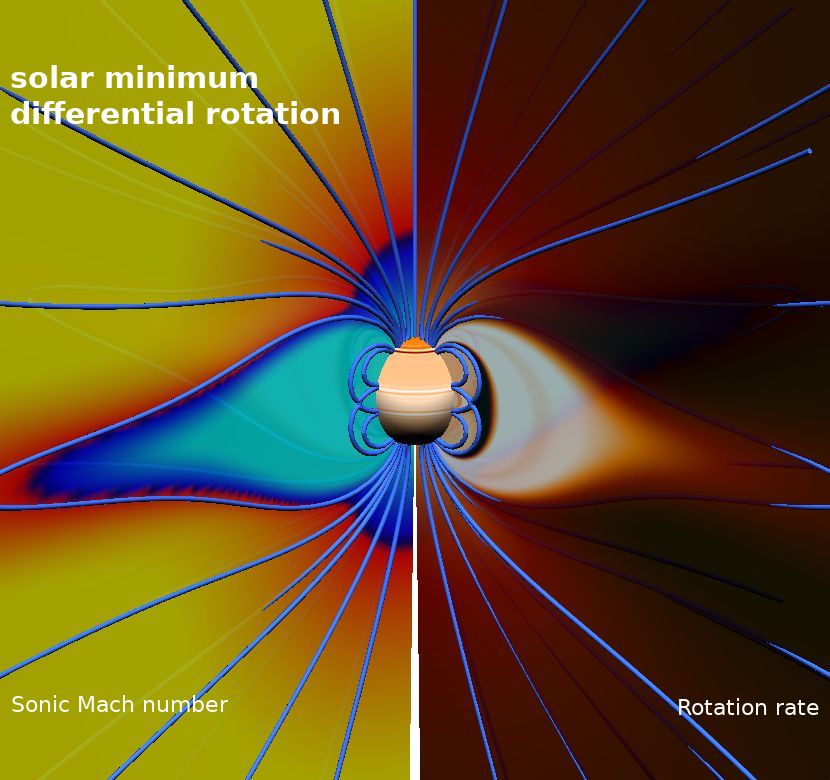
A&A 653, A92 (2021)

Fig. 1. Coronal magnetic field, wind velocity, and rotation rate at three illustrative moments of the solar cycle (from left to right: solar minimum,
maximum, and decay phase, corresponding to instants t = 0, 3.8, and 4 yr in Fig. 3 of Pinto et al. 2011). The left halves of the panels show
meridional slices of the wind speed (sonic Mach number from 0 in solid blue to 2 in solid yellow, and with the yellow–blue boundary representing
the sonic surface), and the right halves show slices of the rotation rate of the solar corona (from 0 in black to 14◦ /day in light orange). Top and
bottom rows correspond to cases with a standard differential rotation and to solid-body rotation at the lower boundary (the lower boundary of the
corona is coloured with the same Ω colour scale as the slices on the right side of the images). Blue lines represent magnetic field lines. The frame
of reference is inertial (not co-moving with the Sun), hence Ω is positive everywhere.

boundaries) progressively develop a backward bend (opposed to               those represented in Fig. 1 (from left to right: solar minimum,
the direction of rotation). The open field lines that pass close to         maximum, and decay phase; differential surface rotation on the
the coronal hole boundaries suffer stronger expansions and devi-            top row, solid-body rotation on the bottom row). The red curves
ations from the radial direction, drive the slowest wind flows,             indicate the rotation period imposed at the surface (Eq. (6), with
and acquire the lowest rotation speeds at mid-coronal heights               Ωb and Ωc having values of 0 in the solid-body rotation case).
(not very far from the streamer tips). Nevertheless, the rotation           The rotation regimes of coronal holes and closed-field regions
rates remain high at and immediately above the streamers tips               are clearly distinct, with the former tending to progressively
(close to the HCS–HPS), as these tend to assume a rotation pro-             approach solid-body rotation with increasing altitude (please
file more closely linked with that of the surface (and of the cor-          note that the case in the third column has pseudo-streamers at
responding streamers). As a result, the strongest spatial contrasts         the north and south poles), and the latter showing a more com-
in wind speed and rotation rate Ω are usually found across these            plex rotation structure. The direct imprint of the imposed sur-
regions of the corona.                                                      face profile is only observed within the first few solar radii, with
                                                                            the overall latitudinal trend of the rotation period (equator to
                                                                            poles) even reversing in the high corona in some cases (e.g.,
2.3. Varying surface rotation profiles and cycle phase
                                                                            in the first and third columns of the figure). Remarkably, rota-
Different surface rotation profiles lead to qualitatively similar           tion periods peak strongly just outside CH–streamer boundaries.
results, with differences between the differentially rotating and           These peaks are present along the entire extent of the bound-
solid-body cases being more pronounced on large coronal loop                aries (we note how they get closer together with increasing alti-
systems. Streamers that are fully rooted at mid- or high latitude           tude, especially for the cases with large streamers), and even
(i.e., not equator-symmetric) are subject to footpoint shearing             beyond, and their positions correspond to the slowing down of
(albeit shallow in amplitude), and acquire an orientation that is           the rotation rate visible as dark patches in the right halves of
oblique in respect to the meridional plane (which does not hap-             the panels in Fig. 1. These features are particularly prominent
pen with solid-body rotation). The positions and amplitudes of              in the solar minimum configuration, with a very large equato-
the fast and slow wind streams do not change when switching                 rial streamer, and are strikingly consistent with the solar coronal
between the two types of rotation. The positions of the higher              rotation periods measured below 2 R by Giordano & Mancuso
and lower rotation-rate regions are also maintained, but their              (2008) using SoHO/UVCS data (during activity minimum from
amplitudes and substructure can differ significantly.                       May 1996 to May 1997). The observations of these latter authors
     Figure 2 shows the rotation period (in days) as a func-                highlight that, as in our simulation, the larger gradients of rota-
tion of latitude at different radii (r = 1.03, 2.0, 4.0, 8.0 and            tion rate are found at the boundaries between open and closed
16 R , from darker to lighter green lines) for the same runs as             magnetic field lines. Furthermore, our simulations suggest that

A92, page 4 of 13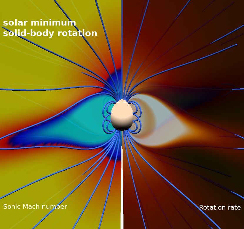
R. F. Pinto et al.: Solar wind speed and rotation shear in the corona

Fig. 2. Rotation period as a function of latitude at different solar radii (r = 1.03, 2.0, 4.0, 8.0 and 16 R , from darker to lighter green lines) for the
runs represented in Fig. 1 (from left to right: solar minimum, maximum, and decay phase; differential surface rotation on the top row, solid-body
rotation on the bottom row). The red curves indicate the rotation period imposed at the surface (Eq. (6), with Ωb and Ωc having values of 0 in the
solid rotation case). Rotation periods peak just outside CH–streamer boundaries, as in the UVCS observations by Giordano & Mancuso (2008).
Global (resonant) oscillations of closed loops within the streamers are visible within these main peaks, especially in the case with differential
rotation. Maximum rotational shearing occurs at mid-altitudes (below maximum streamer height). Wind shear is transmitted upwards, well above
the streamer heights, at the vicinity of HCSs. At greater heights, the corona tends to progressively approach solid-body rotation with height within
coronal holes (please note that the case in the third column has a polar pseudo-streamer).

this behaviour is universal across the activity cycle, although               circle around the Sun (CCW on the pole-on view), while those
less easy to distinguish during solar maximum (cf. second col-                connected to solar wind streams extend outward. Among the lat-
umn in Fig. 2) because of the more intricate mixture of smaller               ter, those that are farther away from the CH–streamer bound-
streamers/pseudo-streamers and thinner coronal holes. This solar              ary cross the domain faster and follow a straighter path, while
minimum-to-maximum variation is also consistent with the                      those that pass closer to it also accelerate slower and suffer a
results of Mancuso & Giordano (2011), who performed a similar                 larger azimuthal deviation before they join the bulk of the wind
analysis with UVCS data during solar maximum (March 1999 to                   flow above. Some flows transition between the two regions, espe-
December 2002). Global (resonant) oscillations of closed loops                cially those passing very close to the interface for which diffu-
within the streamers are visible in the interval between these                sive processes favour that transition. The side view (second row)
main peaks in rotation period (i.e., within streamers), especially            also shows that, in the region that develops the strongest mag-
in the cases with differential rotation. While latitudinal gradi-             netic and flow shear, the coronal rotation makes the equatorial
ents in rotation rate tend to be maximal at mid-altitudes (below              streamer slightly taller and with a sharper transition to the neigh-
maximum streamer height), they remain significant far beyond                  bouring coronal holes.
the height of the largest streamers, in the vicinity of HCSs. The
gradients in rotation period are steeper overall in the cases under
                                                                              2.5. Wind shear near the coronal hole boundaries and on the
differential surface rotation than in the cases with solid-body sur-
                                                                                   extended corona
face rotation.
                                                                              The CH–streamer interface region combines two mechanisms
2.4. Shear flow morphology                                                    that generate shearing flows: one that acts on the meridional
                                                                              plane (caused by the transition from the inner streamer stag-
In order to better show the form and amplitude of the shearing                nant flow to the slow wind region, and finally to the fast wind),
flows imposed by the global coronal rotation, Fig. 3 displays a               and another one that translates into changes in the azimuthal
series of velocity streamlines (or flow lines) corresponding to               component of the flow velocity (caused by the different rota-
flows passing above and below the CH–streamer interface (from                 tion regimes on each side of the boundary). Figure 4 shows the
streamer mid-height to top). For comparison, the plots to the left            absolute values of the gradients of the wind speed (top) and Ω
show a non-rotating solar wind solution, while the plots to the               (bottom) in the low corona during solar minimum (left) and solar
right show the solar minimum configuration with solar-like dif-               maximum (right), focusing on the low-latitude regions. In abso-
ferential rotation. Three perspectives are presented: a front view,           lute terms, flow shear is maximum in the broad regions around
a side view, and a pole-on view (from the north pole), all in the             the CH–streamer interfaces that extend partially into the close-
inertial (not rotating) reference frame. All streamlines are inte-            field regions and into the coronal holes. These broad regions
grated for the same physical time interval, such that the length              of strong shear clearly extend upwards, surrounding the HCSs.
of each streamline indicates the total displacement of a given                The closed-field side of the shear region encloses the transition
fluid element during that period of time. Streamlines that corre-             from the solidly rotating but windless part of the domain to the
spond to plasma lying well within the streamer make an arc of a               slow wind zone, while the open-field side covers the transition

                                                                                                                                      A92, page 5 of 13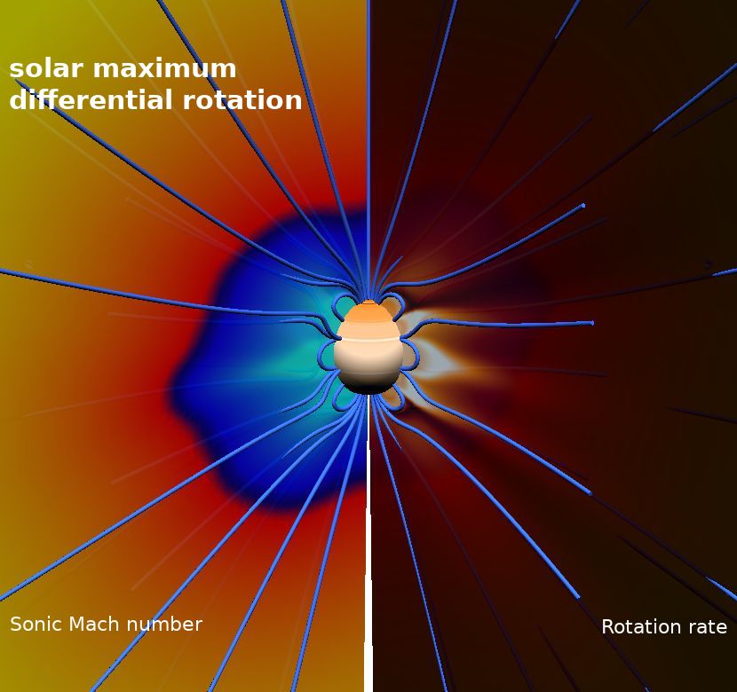
A&A 653, A92 (2021)

Fig. 3. Flow lines for the non-rotating (left) and rotating (right) cases, rendered from different perspectives (from top to bottom: front, side, and
pole-on views). For visual clarity, only the streamlines crossing the northern hemisphere are shown in the front view. The length of each streamline
indicates the total displacement of a given plasma element during the same period of time. Streamlines that correspond to plasma lying well within
the streamer make an arc of a circle around the Sun (CCW on the pole-on view), while those connected to solar wind flows extend outward.

from slow to fast solar wind flow (with decreasing rotation rates).         in and out of the meridional planes represented in Fig. 1. Open
These shearing layers are longer and thicker on the solar mini-             field lines bend backwards, as expected, and more strongly in the
mum configuration, which comprises a large equatorial streamer.             slow wind parts, while the closed loops on the other side of the
The contribution of coronal rotation to the overall shear is more           interface are close to solid-body rotation. From the high corona
clearly visible in the bottom row of the figure. Strong gradients           upwards, the transverse (azimuthal) component of the magnetic
of Ω are found to be more tightly concentrated around the inter-            field grows in amplitude with growing distance from the Sun in
face layers. However, these gradients extend sideways well into             response to solar rotation, as expected from classic wind the-
the coronal holes, and upwards aside HCSs and along the axes                ory. Conversely, the azimuthal component of the velocity field
of pseudo-streamers (see the two mid-latitude pseudo-streamer               can be significant in the low corona, but decreases asymptoti-
structures in the right panels of Fig. 4). In addition, current den-        cally in the high corona. Figure 5 shows the spatial distribution
sity (∼∇ × B) also accumulates at the coronal hole–streamer                 of the ratios between the azimuthal and the poloidal compo-
boundaries, at the streamer tip, and along the HCS. Plasma β                nents of the velocity and of the magnetic field vectors (uφ /u(r,θ)
increases with height along the interface, eventually becoming              and Bφ /B(r,θ) , in absolute value). High values correspond to high
larger than 1 close to the streamer tip (and the base of the HCS).          pitch angles, defined as the angle between the vector and the
    Angular deviations of magnetic field lines relative to the              meridional plane, or the angular deviation in respect to a purely
meridional plane (caused by rotation) are small at these heights            poloidal flow (in r and θ). A non-rotating corona displays null
and therefore hard to visualise directly. But they are present              values everywhere. A rotating corona will contain closed-field
nonetheless, and some of the plotted field lines can be seen to go          regions in (quasi) solid-body rotation with very high uφ /u(r,θ)

A92, page 6 of 13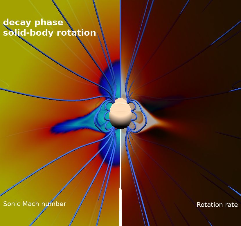
R. F. Pinto et al.: Solar wind speed and rotation shear in the corona

                                                           Wind speed gradient |∇u|

                                                          Rotation rate gradient |∇Ω|

Fig. 4. Zoomed-in view of the absolute magnitudes of the gradients of flow speed (top) and of the rotation rate Ω (bottom) close to the equatorial
streamer on the solar minimum (left) and maximum (right) configurations. For simplicity, only differentially rotating cases are shown, and both
quantities are displayed in normalised units (in units of 6.27 × 10⁻⁴ s−1 and 9.0 × 10⁻¹³ rad s−1 m−1 , respectively). The axis indicates distances
in solar radii. The green lines are magnetic field lines. The coronal hole–streamer boundaries systematically develop flow shears because of the
gradients the solar wind speed (flow along the magnetic field) and of the gradients in the rotation pattern (flow across the field) combined. These
shearing regions reach well into the coronal holes, and into the wind flow well past the streamer top height.

and Bφ /B(r,θ) ≈ 0, and open-field regions for which uφ /u(r,θ)            and fast wind flows and of windless closed-field regions. Stream-
decreases and Bφ /B(r,θ) increases with altitude. Magnetic field-          ers (and generally closed-field regions) have a strong rotational
lines are represented as green lines. Some magnetic features,              signature that is present up to their boundaries. The accelerat-
such as the pseudo-streamers on the case represented in the right-         ing wind flows that surround them rapidly reach speeds high
hand panels, generate localised enhancements of the transverse             enough to overcome the azimuthal (rotational) speeds, and most
(azimuthal) fields that are felt across the radial extent of the           of the coronal hole vorticity becomes dominated by wind speed
numerical domain.                                                          shear. However, some coronal regions develop a strong and
     The combination of flow shears in the meridional and                  extended rotation-induced vorticity signature. The most remark-
azimuthal directions acts as a persistent source of flow vortic-           able examples are pseudo-streamers located at mid-latitudes,
ity (defined as ∇ × u), also with multiple components. Pure wind           which develop elongated rotational shearing zones along their
speed shear due to variations in the radial and latitudinal com-           magnetic axis, as shown in the bottom right panel of Fig. 6.
ponents of the wind speed gradients translates into an azimuthal           These structures separate regions of the corona filled with mag-
vorticity vector that represents vortical motions contained within         netic field rooted at very different latitudes (polar and quasi-
the (r, θ) plane. On the other hand, spatial variations in the             equatorial CHs) with rather different surface rotation rates. Flow
azimuthal speed due to rotation produce a vorticity vector with            shear remains predominantly forced by global rotation through
only radial and latitudinal components (poloidal vorticity), cor-          large distances on these layers, and thus developing a mainly
responding to vortical flows that develop in the (θ, φ) or in the          field-aligned vorticity (corresponding to vortical motions orthog-
(r, φ) planes. Figure 6 shows the spatial distributions of the abso-       onal to the main magnetic field orientation).
lute values of flow vorticity (top) and the ratio of the poloidal to
azimuthal vorticity (i.e., ratio of rotation-induced to wind-speed-
induced vorticities; bottom plots). Left and right columns show            3. Sun–Parker Solar Probe connectivity context
the differentially rotating cases at solar minimum and at solar
maximum, as in the previous figures. Flow vorticity is maxi-               In order to establish links between the results of our numeri-
mal at the interfaces between closed and open magnetic field, as           cal simulations and measurements made by PSP, we attempted
can be guessed from Figs. 4 and 5, and extends outward around              to determine the source regions of the wind streams detected
streamer and pseudo-streamer stalks. The yellow regions in the             in situ, together with their trajectories across the solar corona.
bottom plots indicate zones where the poloidal component – the             This allowed us to verify the applicability of the model to
one that is rotation-induced and can give rise to field-aligned vor-       the coronal context at play, and hence to determine the phys-
ticity – is predominant. Conversely, the pink areas are dominated          ical conditions most likely experienced by those solar wind
by wind speed shear caused by the spatial distributions of slow            flows.
                                                                                                                                A92, page 7 of 13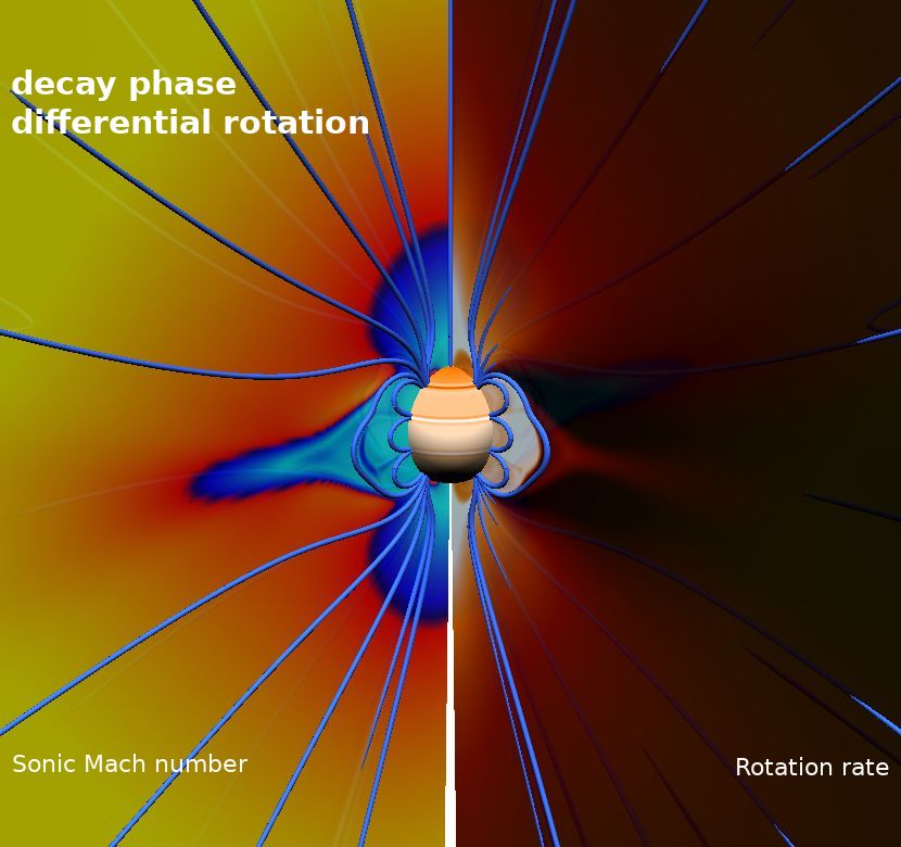
A&A 653, A92 (2021)

                                                                 uφ to u(r,θ) ratio

                                                                 Bφ to B(r,θ) ratio

Fig. 5. Ratio of azimuthal to meridional vector components of the velocity (top) and magnetic field (bottom) for the solar minimum (left) and solar
maximum (right) configurations. Distances are in solar radii, and green lines are magnetic field lines. For simplicity, only differentially rotating
cases are shown. The cores of closed-field regions display high uφ /u(r,θ) ratios and Bφ /B(r,θ) ≈ 0 due to them being in solid-body rotation. Open-
field regions develop a uφ /u(r,θ) profile that decays with altitude while Bφ /B(r,θ) grows. Coronal hole–streamer boundaries show stark contrasts in
velocity and magnetic-field pitch angles, and also extend coronal regions above the mid-latitude pseudo-streamers on the right panels.

                                                            Flow vorticity |∇ × u|

                           Ratio of poloidal (rotation-induced) to azimuthal (parallel flow induced) vorcity

Fig. 6. Unsigned flow vorticity (top) and ratio of poloidal to azimuthal vorticity components (bottom) in the low-latitude regions for the solar
minimum and solar maximum configurations. For simplicity, only differentially rotating cases are shown and flow vorticity is displayed in nor-
malised units (9.0 × 10⁻¹³ rad s−1 m−1 ). The axes indicates distances in solar radii. Green lines are magnetic field lines. The combination of the
shearing flows in Fig. 4 is a source of vorticity that extends along the CH–steamer boundaries and above. The yellow regions in the bottom plots
indicate zones where the poloidal component (the only one that gives rise to field-aligned vorticity caused by gradients of vφ produced by coronal
rotation) is predominant. Pink areas are dominated by wind speed shear (rather than rotational shear). Streamers have a strong rotational signature.
Pseudo-streamer axes display elongated rotational shearing zones.

A92, page 8 of 13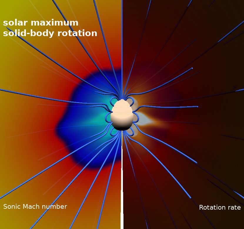
R. F. Pinto et al.: Solar wind speed and rotation shear in the corona
3.1. The Connectivity Tool 3.2. Sun-to-spacecraft connectivity, solar wind trajectories
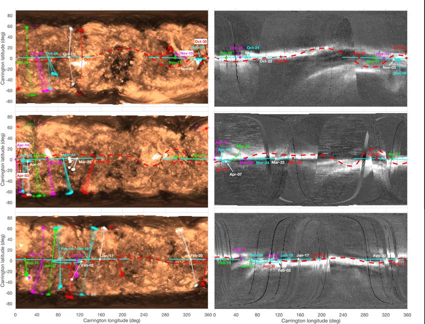
Figure 7 shows the trajectory of PSP during perihelia 1, 2,
We used the IRAP Connectivity Tool1 to determine the most and 4 (thick black line on the left, green on the right pan-
probable paths taken by the solar wind streams all the way els) plotted over Carrington maps of coronal extreme ultraviolet
from the solar surface to the position of PSP during its first
four perihelia. The connectivity tool calculates the magnetic and (EUV) emission (SDO/AIA 193 Å; first column) and white-
solar wind connectivity between the Sun and different space- light emission at 5 R (SoHO/LASCO C3; second column). The
craft (or Earth) continuously, so as to establish physical links corresponding time periods are during October–November 2018
between them, all along their orbits (Rouillard et al. 2020b). (top), March–April 2019 (middle), and January–February 2020
The tool offers different possible sources of input magnetogram (bottom). Pale blue and red layers cover the base of coronal holes
data, extrapolation methods, and wind propagation models, and with positive and negative polarity, respectively. The coloured
allows the user to assess uncertainties and inconsistencies related symbols represent the positions of the solar wind plasma that
to the measurements and models used. We chose to setup the reached PSP computed using the IRAP connectivity tool, with
Connectivity Tool with standard Potential Field Source–Surface in situ measurement dates labelled in corresponding colours.
(PFSS) extrapolations of Air Force Data Assimilative Photo- Stars indicate the solar wind plasma position at the PFSS source-
spheric Flux Transport (ADAPT) magnetograms (Arge & Pizzo surface altitude (only the centroid of the uncertainty ellipse
2000; Arge et al. 2003). It also provides an evaluation of the is shown for simplicity), and circles indicate the most likely
PFSS reconstructions by comparing the topology of the neutral wind source positions at the solar surface. The dotted lines that
line with that of streamers (Poirier et al. 2021). The choice of connect them are visual aids and for simplicity do not trace
the ADAPT magnetograms was based on this evaluation proce- the actual field-line trajectories. Following the description in
dure. Propagation paths and temporal delays were determined Sect. 3.1, each star corresponds to several circles that indicate
by adjusting a solar wind profile to the wind speeds measured the scatter due to mapping uncertainties. The red dashed line rep-
at the position of PSP at each moment of its trajectory. The resents the neutral line (base of the HCS) obtained from PFSS
wind velocities were obtained from the SWEAP instrument suite extrapolation of ADAPT/GONG maps. We excluded the third
(Kasper et al. 2016), and particularly from the plasma moments PSP encounter because of the unavailability of continued good-
from the Solar Probe Cup (SPC; Case et al. 2020). The solar quality solar-wind data during the corresponding time interval.
wind mapping from the spacecraft position to the low corona, The surface footpoint charts overlaid on the EUV 193 Å
and from there to the surface, can be affected by different sources synoptic maps indicate that PSP spent a significant fraction
of error. Uncertainties related to the exact wind acceleration pro- of its first passages sampling solar wind streams that devel-
file can lead to different solar wind propagation paths, and hence oped at the vicinity of predominantly azimuthaly aligned CH–
to deviations in longitude in the high corona, and total wind streamer boundaries. These regions correspond topologically to
travel time. PFSS extrapolations from magnetic fields measured the boundary shear layers illustrated in the top-left panel of
at the surface of the Sun are furthermore occasionally affected by Fig. 4 (for our simulated solar minimum case). The mappings at
positional errors that translate into latitudinal deviations of the 5 R in the right panels (white-light maps) show that the streams
coronal structures of a few degrees. In order to cope with these detected by PSP propagated through the heliospheric plasma
issues, the Connectivity Tool determines the points at the sur- sheet (in close proximity to the HCS), and through the bright
face of the Sun that connect to an uncertainty ellipse around the streamer-belt region. This region corresponds to the equatorial
orbital position of the target spacecraft (covering the expected regions in the high corona in our solar minimum simulations,
latitudinal and longitudinal uncertainties). For any given time, just above the tip of the large equatorial streamer.
the tool therefore provides a list of surface footpoints with dif- Solar wind connectivity across this range of heliocentric dis-
ferent associated probabilities rather than unique positions. The tances (1 to 5 R ) is better shown in Fig. 8 for one selected
time period covered by the present paper corresponds to solar instant (during the second PSP encounter). The figure shows a
minimum configuration, with a close-to axi-symmetric corona three-dimensional rendering of the global magnetic field struc-
and a rather flat HCS. As a result, the dispersion of the foot- ture of the corona on March 23 2019 (cf. Fig. 7) and the mag-
point positions predicted for any given date and time leads to netic field lines through which the wind plasma that reached PSP
a region that is very elongated in the azimuthal direction, with at the instant represented is likely to have escaped from before-
the corresponding errors rarely leading to topologically differ- hand. The two panels show side and top views, as in Fig. 3
ent regions of the Sun. This also holds for moments when the (middle and bottom panels) for our solar minimum MHD sim-
spacecraft is in close proximity to the HCS and the expected ulations. The ADAPT/GONG magnetogram used on our coro-
footpoints split into both solar hemispheres (northern and south- nal field reconstruction is plotted over the surface of the Sun,
ern end-regions are topologically similar). We also made extra with green and red shades representing positive and negative
runs with lower and higher solar wind speeds for the duration polarities. The transparent grey surface represents the bound-
of the time-periods analysed and found that the properties of the ary between the large equatorial streamer and the polar coro-
connected regions do not change significantly. Our aim here is to nal holes, and the violet ribbon indicates the base of the HCS
identify the types of solar wind source regions (in the topological (polarity inversion line). Light yellow lines represent a series of
sense) rather than exact surface footpoint coordinates. Therefore, magnetic field lines that sample the whole uncertainty ellipse
the error sources described above do not translate into variations taken into account by the Connectivity Tool. A fraction of these
of the dynamical and topological properties of the regions lines map towards the base of the coronal hole on the north-
crossed by the solar wind, and therefore should not affect our ern hemisphere, but are discarded because they correspond to an
analysis. opposite magnetic polarity to that measured in situ by PSP. The
dark red lines indicate the connectivity paths ranked with the
highest connectivity probability. The blue lines trace a few addi-
tional open field lines rooted inside coronal holes. It is clear from
1
http://connect-tool.irap.omp.eu/ the figure that the wind streams sampled by PSP at this instant
A92, page 9 of 13
A&A 653, A92 (2021)

Fig. 7. Sun-to-PSP connectivity maps for the first (October–November 2018), second (March–April 2019), and fourth (January–February 2020)
encounters (top, middle, and bottom row, respectively). Connectivity is computed by projecting the solar wind speed measured at PSP back-
wards to the surface of the Sun, considering the most likely Parker spiral, accounting for solar wind travel time and connecting to coronal field
reconstructions based on magnetograms corresponding to the expected solar wind release times. The left panels display Carrington maps of EUV
emission (SDO/AIA 193Å) overlaid with the most probable footpoints (solar wind source positions, coloured circles) at the surface of the Sun for
the dates indicated, and the centroid of the connectivity probability distribution at 5 R (coloured stars). The cyan line indicates the trajectories of
the 2.5 R connectivity point. The coloured dotted lines are visual aids to connect source-surface to surface positions (but do not trace the actual
field-line trajectories). Date labels indicate in situ solar wind measurement times. The right panels show similar maps of white light emission at
5 R (SoHO/LASCO C3), overlaid with similar markers (at 5 R ). The red dashed line represents the neutral line (base of the HCS) obtained from
PFSS extrapolation of ADAPT/GONG maps. PSP spent a significant fraction of its first passages sampling solar wind streams that developed at
the vicinity of predominantly azimuthally aligned CH–streamer boundaries, and that propagated through the heliospheric plasma sheet (in close
proximity to the HCS, within the bright streamer belt region).

developed along paths that closely delineate azimuthaly aligned              of azimuthally aligned CH–streamer boundaries, and especially
CH–streamer boundaries, in concordance with the MHD simu-                    so during the second and fourth encounters, with occasional con-
lations discussed in Sect. 2. In view of the temporal sequence               nections to small low-latitude coronal holes or equatorward polar
of Sun-to-PSP solar wind connectivity displayed in Fig. 7, this              coronal hole extensions (Griton et al. 2021). The solar corona
configuration was the most common one throughout the periods                 retained a high degree of axial symmetry throughout the time
analysed.                                                                    periods involved in this analysis. The HCS (and HPS) main-
    The most probable Sun–spacecraft solar wind propagation                  tained a predominant E–W orientation in the solar regions con-
paths lie, for the most part, along the boundary between the                 nected to PSP. These reasons justify the use of the MHD sim-
large equatorial streamer and the polar coronal holes. As PSP                ulations represented in Figs. 1–6. This is especially true for
proceeded on its orbit, the source regions at the surface scanned            the solar minimum case (with an axi-symmetric large equato-
this boundary continuously, apart from during brief periods of               rial streamer). Deviations from this configuration, such as the
connection to low-latitude coronal holes or to deep equatorward              coronal hole extensions and equatorial coronal holes visible near
polar CH extensions. PSP spent a large fraction of its first few             Carrington longitudes 280 and 80 in Fig. 7, are in principle asso-
encounters probing solar wind streams that formed in the vicinity            ciated with pseudo-streamers such as those in our simulations

A92, page 10 of 13
R. F. Pinto et al.: Solar wind speed and rotation shear in the corona
Fig. 8. Three-dimensional rendering of the Sun-to-PSP connectivity paths on March 23 2019 at 00:00 UT, during the second encounter with
PSP (cf. middle panels of Fig. 7). The two panels show side and top views, as in the simulations in Fig. 3 (middle and bottom panels). The
radial component of the surface magnetic field is represented in green (positive polarity) and red (negative polarity) tones, retrieved from the
same ADAPT/GONG magnetograms as in the previous figure. The transparent grey surface represents the boundary between the large equatorial
streamer and the polar coronal holes, and the violet ribbon indicates the base of the HCS. The light yellow lines cover the whole uncertainty ellipse
taken into account by the Connectivity Tool. A fraction of these lines map towards the northern hemisphere, but can be discarded because they
correspond to the opposite magnetic polarity to that measured in situ by PSP (although they fall into topologically and dynamically equivalent
regions of the corona). The dark red lines indicate the connectivity paths ranked with the highest connectivity probability. The blue lines trace a
few additional open field lines rooted inside coronal holes. PSP is connected to field lines (and wind streams) that closely delineate azimuthaly
aligned CH–streamer boundaries, in concordance with the MHD simulations discussed in Sect. 2. All the lines (that sample the whole uncertainty
ellipse) clearly fall into compact regions that correspond to the broad shearing zones in the top-left panels of Figs. 4 and 6.
for the cycle decay phase (right panels of Figs. 4–6, at mid- orientation of the equatorial streamer observed during this period
latitudes), although perhaps with different sizes and orientations. and that of our simulations, on which streamer–CH boundaries
We consider that the regions rooted at about ±60 deg in our are parallel to the direction of rotation. While less favourable to
simulations for the solar minimum case (cf. Figs. 4–6, left) are interchange reconnection, this spatial orientation does not ham-
the most representative of the source regions of the wind flows per the formation of the shear flows in the solar wind shown in
detected by PSP. These are coronal hole boundary regions ori- Figs. 3–6. Furthermore, these shears remain visible up to large
ented in the east–west direction (parallel to the direction of solar heliocentric distances, which could favour the propagation (or
rotation). Solar wind streams originating from these regions are even amplification) of magnetic perturbations formed in the low
accelerated through an environment with significant and spa- corona, allowing them to survive more easily up to the altitude of
tially extended solar wind speed and rotation shear, and corre- detection (Owens et al. 2020; Macneil et al. 2020). Beyond this
spond to the peaks in rotation period in the left panels of Fig. 2. phenomenology, the boundaries of polar coronal holes are also
The dynamical properties of these zones of the corona should known to be highly dynamic and to undergo significant recon-
have an impact on the properties of the wind measured in situ, figuration over the roughly 24-hour timescale of supergranules
and could be responsible for some of their characteristics. On (Wang et al. 2010). These effects are not modelled in this paper,
PSP data, transitions from streamer (i.e., boundary layer) to non- but could induce additional variability that could be measured by
streamer (core of coronal hole) wind flows were accompanied PSP. The existence of neighbouring solar wind streams with dif-
by a clear decrease in the variability of the wind (Rouillard et al. ferent rotation rates (such as those in the streamer stalk regions
2020a), both in frequency and amplitude of magnetic SBs, and a on our simulations) should furthermore contribute to increasing
decrease in the occurrence of strong density fluctuations. This the variability of the transverse (rotational) velocities measured
suggests that the physical conditions associated with coronal by PSP, especially as the HCS is slightly warped (cf. Fig. 7).
hole boundaries are favourable to the development of such per-
turbations. Interchange reconnection, often invoked as a possi-
ble SB generation mechanism (Fisk & Kasper 2020), relies on 4. Conclusion
the forcing of these boundary regions by the large-scale rotation 4.1. Summary
of the corona. However, it is expected to be enhanced (or more
efficiently driven) at CH–streamer boundaries that are orthog- We investigate the development of spatially extended solar wind
onal or inclined with respect to the direction of rotation, as a shear regions induced by solar rotation and by variations in solar
streamer pushes into neighbouring CHs for example (see e.g., wind speed, following recent PSP results. Our analysis com-
Lionello et al. 2005), and reduced on azimuthally aligned CH– bines simulations made using a MHD numerical model of the
streamer boundaries. This is in contrast to the general spatial solar wind and corona and estimations of the sun-to-spacecraft
A92, page 11 of 13A&A 653, A92 (2021)
connectivity during the first four PSP solar encounters to aid in transmitted to the corona in a complex manner that depends
associating model results to spacecraft data. Our main findings intrinsically on the organisation of the large-scale magnetic field
are as follows. at any given moment. Coronal rotation is highly structured at
1. Solar wind flows that develop in the vicinity of coronal hole low coronal altitudes, with a clear signature of slowly rotat-
boundaries are subject to persistent and spatially extended ing flows that follow the CH–streamer boundaries, in agreement
shearing. There are two components to this shearing: a wind with the observations by Giordano & Mancuso (2008). Some of
speed shear due to the transition from closed-field (no- these strong gradients in rotation rate produce an imprint that
wind) to the slow and fast wind regions, and a rotational extends far into the high corona (up to the upper boundary of
shear due to the way coronal rotation settles in response the numerical model). These non-uniformities in rotation rate
to the rotation of the solar surface. The most significant translate into solar wind flow shear with a vorticity component
shearing occurs in thin layers that lie along CH–streamer oriented along the magnetic field and solar wind propagation
(or pseudo-streamer) boundaries, and that stretch outwards direction, that adds up to the shear caused by the spatial dis-
in the vicinity of HCSs and pseudo-streamer stalks. Wind tribution of fast and slow wind flows (and that can only generate
speed shear generates a spatially broad shearing signature an orthogonal vorticity component).
associated with a large-scale vorticity vector oriented in the The MHD model setup relies on a number of simplifica-
azimuthal direction. Rotational shearing produces shearing tions to the full physical problem; it uses a polytropic descrip-
patterns with field-aligned vorticity that become predomi- tion of the plasma thermodynamics, meaning that the heating
nant in elongated regions above pseudo-streamer stalks that and cooling mechanisms are not modelled in detail, but that
extend to great distances from the Sun. the main dynamical and geometrical features of the solar wind
2. The solar corona acquires a complex rotation pattern that dif- are retained. This approach furthermore leads to a solar wind
fers significantly from that of the surface rotation that drives with speed variations that are much weaker than those found in
it. Closed-field regions (streamers, pseudo-streamers) tend the real solar atmosphere (smaller contrast between typical fast
to set themselves into solid body rotation, with a rate that and solar wind speeds and broader transitions). We settled on
is consistent with that of the surface regions at which they the limiting case in which the rotating solar corona and solar
are rooted. Open field lines show a variety of rotation rates, wind are perfectly axisymetric (with CH–streamer boundaries
with those that pass near coronal hole boundaries acquir- perfectly parallel to the direction of rotation). Rotation-induced
ing the lowest rotation rates at mid-coronal heights, in stark interchange reconnection is completely inhibited in this config-
contrast with the closed-field regions across the boundary. uration, as is the development of shear instabilities. The forma-
This results in clear increases in rotation period adjacent to tion of full vortical flows in the (θ, φ) plane and the injection of
streamers (especially visible in large streamers), in agree- helicity into the wind flow are inhibited. However, this choice
ment with SoHO/UVCS observations. Streamer stalks (and of problem symmetry has a number of advantages in respect to
the vicinity to HCS/HPS) can contain a mixture of wind the full 3D equivalent, namely that it allows many more varia-
streams at different rotation rates (slow rotating flows com- tions of parameters to be run (different phases of the cycle, dif-
ing from the CH boundaries, faster wind flows coming from ferent solar surface rotation profiles), and that the runs can be
the streamer tips). easily made at a higher spatial resolution. As a consequence, the
3. Solar wind flows probed by PSP during its first four orbits simulations develop sharper CH–streamer boundaries than their
form and propagate away from the Sun through regions full-3D counterparts, which helps to make the rotation shears
of enhanced wind speed and rotational shear. Our Sun- more apparent. These boundaries should nevertheless be much
to-spacecraft connectivity analysis shows that such solar sharper in the real solar corona. For these reasons, the ampli-
wind flows originated mostly at the boundaries of quasi- tudes of solar wind speed and rotational shearing layers should
axisymetric polar coronal holes, with occasional crossings of be higher in the real Sun than those that the MHD simulations are
low-latitude coronal holes. The measured wind flows showed capable of producing. We also used an idealised solar dynamo
a strong and complex rotational signature permeated by per- model to constrain the large-scale magnetic field topology at
vasive magnetic perturbations such as SBs (among others). each moment of the solar cycle, meaning that our MHD simu-
Our results suggest that the slow wind flows detected by lations are not designed to model a specific event, but rather to
PSP should experience persistent shears across their forma- help us to understand the dynamics of the regions of interest (the
tion and acceleration regions, supporting the idea that these model produces a full set of typical solar coronal structures –
should have an impact on the formation of localised mag- streamers, pseudo-streamers, and coronal holes – placed at dif-
netic field reversals and be favourable to their survival across ferent latitudes according to solar activity).
the heliosphere. As we have shown with the help of the IRAP Connectivity
Tool2 , the solar wind streams that reached PSP during its first
few encounters most often traversed the vicinity of the bound-
4.2. Discussion and perspectives
aries between a large equatorial streamer and the adjacent coro-
Unlike for the photospheric counterpart, our current knowledge nal holes. The dynamics at play in such regions suggest that
of the rotational state of the solar corona is very limited. Dif- they are potential hosts for the development of shearing insta-
ferent observation campaigns (relying on different measurement bilities (among others), which are continuously driven by the
methods) have suggested that the corona rotates in a manner that large-scale wind shears at these boundaries. Such processes can
is not in direct correspondence with the surface rotation, and potentially introduce alfvénic perturbations into the solar wind
that it depends to some degree on the solar cycle phase (i.e., and/or give rise to discrete helical (and pressure-balanced) MHD
on the global magnetic topology). More recently, PSP unveiled structures (depending on the aforementioned instability thresh-
the prevalence of strong rotational flows that increase rapidly in olds, growth rates, and timescales of ejection onto the wind).
amplitude as the spacecraft approached the Sun, at least in the Because of the limitations intrinsic to the global MHD approach
regions probed during its first few close passes (Kasper et al.
2019). Our MHD simulations show that surface rotation is 2
http://connect-tool.irap.omp.eu/
A92, page 12 of 13You can also read