Optimization of Solar Sailcraft Trajectory for a Comet Sample Return Mission - Ananthakrishnan Krishnan
←
→
Page content transcription
If your browser does not render page correctly, please read the page content below
Optimization of Solar Sailcraft Trajectory
                           for a Comet Sample Return Mission

                           Ananthakrishnan Krishnan
Master of Science Thesis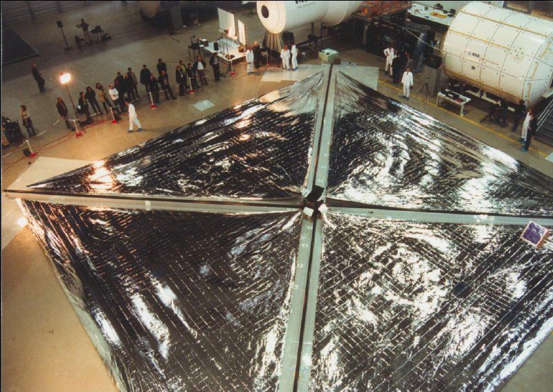
O PTIMIZATION OF S OLAR S AILCRAFT T RAJECTORY
     FOR A C OMET S AMPLE R ETURN M ISSION

                                          by

                        Ananthakrishnan Krishnan

              in partial fulfillment of the requirements for the degree of

                                   Master of Science
                               in Aerospace Engineering

                        at the Delft University of Technology,
          to be defended publicly on Monday December 17, 2018 at 9:00 AM.

           Student number:      4518934
           Thesis committee:    Prof. Dr. E. Schrama,            Chairholder
                                Prof. Ir. R. Noomen,             Supervisor
                                Prof. Ir. B. T. C. Zandbergen,   External

       This thesis is confidential and cannot be made public until June 16, 2019.

 An electronic version of this thesis is available at http://repository.tudelft.nl/.
A CKNOWLEDGEMENTS
Writing this report marks almost the end of my Masters in Aerospace Engineering at TU Delft. My
masters journey, which started as a passion for space exploration, has been a thoroughly exciting
and challenging experience, and to reach this point would not have been possible without all the
wonderful people who supported me during this period.

First of all, I would like to thank my supervisor Prof. Ron Noomen, for giving me the opportunity
to work with him on this topic. I am really grateful for his help, guidance and support throughout
the thesis, which were instrumental for completing it. I would also like to thank him for all the dis-
cussions and conversations during the countless weekly meetings, which kept me motivated during
the course of the thesis.

I would like to express my gratitude to Dr. Dominic Dirkx for his help and support with the devel-
opment of the solar sail model in Tudat. His timely guidance were crucial for solving the coding
related issues that occurred during the thesis. I am also thankful for the invaluable help and sugges-
tions given by Dr. Jeannette Heiligers during the critical phases of my thesis.

My time at Delft would not have been complete without my friends. I thank all my friends for shar-
ing all the amazing and wonderful moments during these three years, the memories of which I will
remember forever. In addition to the fun times, I thank them for helping me through the challeng-
ing phases of my masters as well.

Lastly and most importantly, I am forever grateful to my parents, who are my source of motivation
and strength. I would like to thank them for their unconditional love, constant belief, continuous
support and encouragement during this period.

                                                                         Ananthakrishnan Krishnan
                                                                              Delft, December 2018

                                                 iii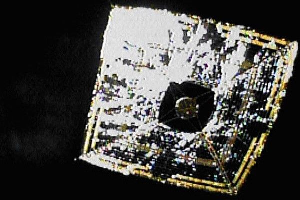
A BSTRACT
Comets, the sporadic visitors from the outer edges of the Solar System, are considered to hold the
key for understanding the formation of planets and the origin of life on Earth. Having spent the
majority of time away from the radiative environment of the inner Solar System, the chemistry of
the comets has remained unaltered, making them the pristine samples of the matter from the an-
cient Solar nebula. A mission to bring cometary particles back to Earth enables the examination of
the materials in well equipped laboratories and saves the mass of the instruments to be carried on
board. To this end, a comet sample return mission has been a priority in the Solar System explo-
ration plans of space agencies. However, due to the highly inclined and highly eccentric nature of
comets’ orbits, it is challenging to reach them. As conventional propulsion methods require a large
quantity of propellant for this type of mission, the feasibility of using the novel propulsion tech-
nique of solar sailing is explored in this thesis. The solar sailcraft is propelled by the reflection of the
incident solar radiation on a large, lightweight sail. In order to return the comet samples to Earth
within a reasonable time period, the orbit transfer is considered as an optimal control problem with
constraints placed on the sailcraft’s position and velocity.

The comet 103P/Hartley 2 was selected as the target for the mission and the total mission (to the
comet and back to Earth) is aimed to be completed within the ten year period between 2020-2030.
A perfectly reflecting (ideal) square sail with a lightness number β of 0.05 (moderate performance)
was considered for the analysis. The sailcraft was to depart from a heliocentric Earth orbit and the
sail orientation was considered to change at a fixed number of nodal points along the trajectory. The
Differential Evolution (DE) algorithm was used to search for time-optimal trajectories that minimize
the approach distance to the comet and the relative velocity with respect to the comet during sample
collection. Grid Search method was used to narrow in on the optimal departure date and time-of-
flight based on the optimization result. The optimal trajectory obtained predicts the solar sailcraft
to reach the comet, collect the samples and return back to Earth in 6.77 years. The time of arrival
at the comet was found to match with the comet’s perihelion passage, enabling effective sample
collection. The outcome of the trajectory analysis, thus successfully demonstrates the applicability
of solar sailing to comet sample return missions in the near future.

                                                     v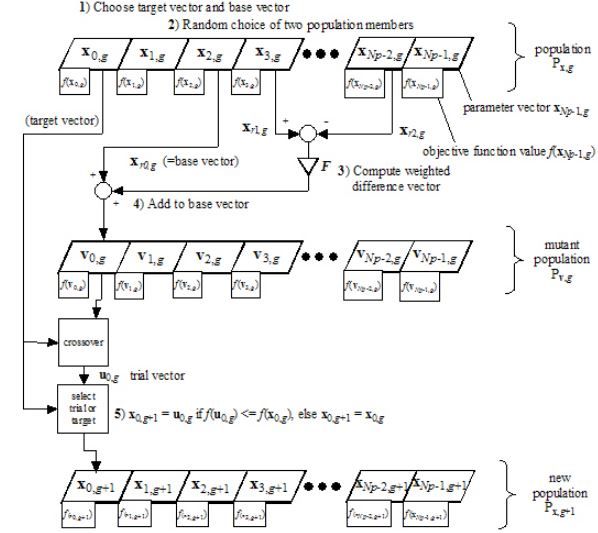
C ONTENTS

Abstract                                                                                                                                                                        v

List of Abbreviations                                                                                                                                                          ix

List of Symbols                                                                                                                                                                xii

1 Introduction                                                                                                                                                                  1

2 Background                                                                                                                                                                    5
  2.1 Heritage of Solar Sailing    .   .   .   .   .   .   .   .   .   .   .   .   .   .   .   .   .   .   .   .   .   .   .   .   .   .   .   .   .   .   .   .   .   .   .    5
  2.2 Missions to Comets . .       .   .   .   .   .   .   .   .   .   .   .   .   .   .   .   .   .   .   .   .   .   .   .   .   .   .   .   .   .   .   .   .   .   .   .    8
  2.3 Mission Objectives . . .     .   .   .   .   .   .   .   .   .   .   .   .   .   .   .   .   .   .   .   .   .   .   .   .   .   .   .   .   .   .   .   .   .   .   .   12
  2.4 Mission Target . . . . .     .   .   .   .   .   .   .   .   .   .   .   .   .   .   .   .   .   .   .   .   .   .   .   .   .   .   .   .   .   .   .   .   .   .   .   13

3 Theory                                                                                                                                                                       15
  3.1 Reference Frames . . . . . . . . . . . . . . . . . . . .                                         .   .   .   .   .   .   .   .   .   .   .   .   .   .   .   .   .   .   15
      3.1.1 Heliocentric Reference Frame . . . . . . . . . .                                           .   .   .   .   .   .   .   .   .   .   .   .   .   .   .   .   .   .   16
      3.1.2 Spacecraft orbital reference frame . . . . . . .                                           .   .   .   .   .   .   .   .   .   .   .   .   .   .   .   .   .   .   16
      3.1.3 Reference Frame Transformation . . . . . . . .                                             .   .   .   .   .   .   .   .   .   .   .   .   .   .   .   .   .   .   17
  3.2 Coordinate Systems . . . . . . . . . . . . . . . . . . .                                         .   .   .   .   .   .   .   .   .   .   .   .   .   .   .   .   .   .   18
      3.2.1 Cartesian Coordinates . . . . . . . . . . . . . .                                          .   .   .   .   .   .   .   .   .   .   .   .   .   .   .   .   .   .   18
      3.2.2 Keplerian Elements. . . . . . . . . . . . . . . .                                          .   .   .   .   .   .   .   .   .   .   .   .   .   .   .   .   .   .   19
      3.2.3 Modified Equinoctial Elements . . . . . . . . .                                            .   .   .   .   .   .   .   .   .   .   .   .   .   .   .   .   .   .   19
  3.3 Dynamics Model . . . . . . . . . . . . . . . . . . . . .                                         .   .   .   .   .   .   .   .   .   .   .   .   .   .   .   .   .   .   20
  3.4 Perturbations . . . . . . . . . . . . . . . . . . . . . . .                                      .   .   .   .   .   .   .   .   .   .   .   .   .   .   .   .   .   .   20
  3.5 Solar Sailing. . . . . . . . . . . . . . . . . . . . . . . .                                     .   .   .   .   .   .   .   .   .   .   .   .   .   .   .   .   .   .   22
      3.5.1 Performance metrics . . . . . . . . . . . . . . .                                          .   .   .   .   .   .   .   .   .   .   .   .   .   .   .   .   .   .   22
      3.5.2 Ideal Sail Force Model . . . . . . . . . . . . . .                                         .   .   .   .   .   .   .   .   .   .   .   .   .   .   .   .   .   .   23
      3.5.3 Optical Sail Force Model . . . . . . . . . . . . .                                         .   .   .   .   .   .   .   .   .   .   .   .   .   .   .   .   .   .   25
      3.5.4 Choice of SRP Force Model . . . . . . . . . . .                                            .   .   .   .   .   .   .   .   .   .   .   .   .   .   .   .   .   .   26
  3.6 Equations of motion . . . . . . . . . . . . . . . . . . .                                        .   .   .   .   .   .   .   .   .   .   .   .   .   .   .   .   .   .   27
      3.6.1 Vector Form . . . . . . . . . . . . . . . . . . . .                                        .   .   .   .   .   .   .   .   .   .   .   .   .   .   .   .   .   .   27
      3.6.2 Gauss’ form of Lagrange’s Planetary Equations.                                             .   .   .   .   .   .   .   .   .   .   .   .   .   .   .   .   .   .   27

4 Numerical Tools                                                                                                                                                              29
  4.1 Integrator . . . . . . . . . . . . . . . . .                     .   .   .   .   .   .   .   .   .   .   .   .   .   .   .   .   .   .   .   .   .   .   .   .   .   .   29
  4.2 Integrator Choice. . . . . . . . . . . . .                       .   .   .   .   .   .   .   .   .   .   .   .   .   .   .   .   .   .   .   .   .   .   .   .   .   .   31
  4.3 Optimization . . . . . . . . . . . . . . .                       .   .   .   .   .   .   .   .   .   .   .   .   .   .   .   .   .   .   .   .   .   .   .   .   .   .   31
      4.3.1 LTOM and GTOM . . . . . . . . .                            .   .   .   .   .   .   .   .   .   .   .   .   .   .   .   .   .   .   .   .   .   .   .   .   .   .   33
      4.3.2 Choice of Optimization Method .                            .   .   .   .   .   .   .   .   .   .   .   .   .   .   .   .   .   .   .   .   .   .   .   .   .   .   34
  4.4 Differential Evolution . . . . . . . . . .                       .   .   .   .   .   .   .   .   .   .   .   .   .   .   .   .   .   .   .   .   .   .   .   .   .   .   35
  4.5 Grid Search . . . . . . . . . . . . . . . .                      .   .   .   .   .   .   .   .   .   .   .   .   .   .   .   .   .   .   .   .   .   .   .   .   .   .   37

                                                                       vii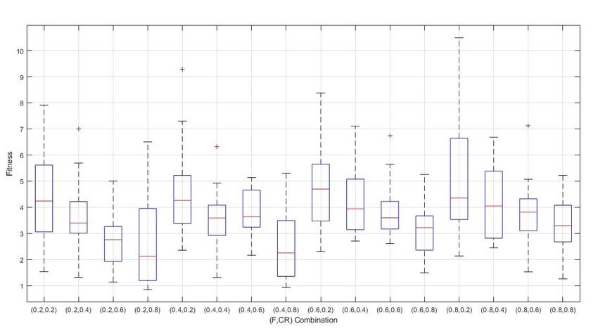
viii C ONTENTS
5 Validation and Parameter Tuning 39
5.1 SRP Acceleration Model Validation . . . . . . . . . . . . . . . . . . . . . . . . . . . . . 39
5.2 Sailcraft Dynamics Validation . . . . . . . . . . . . . . . . . . . . . . . . . . . . . . . . 40
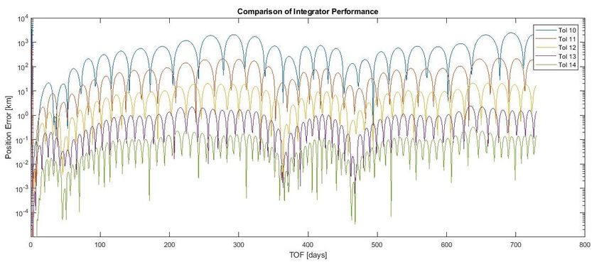
5.3 Integrator Tuning. . . . . . . . . . . . . . . . . . . . . . . . . . . . . . . . . . . . . . . 42
5.4 Integrator validation . . . . . . . . . . . . . . . . . . . . . . . . . . . . . . . . . . . . . 45
5.5 DE Tuning. . . . . . . . . . . . . . . . . . . . . . . . . . . . . . . . . . . . . . . . . . . 46
5.5.1 Objective function . . . . . . . . . . . . . . . . . . . . . . . . . . . . . . . . . . 47
5.5.2 Node Vs Population Size . . . . . . . . . . . . . . . . . . . . . . . . . . . . . . . 48
5.5.3 F and CR combination . . . . . . . . . . . . . . . . . . . . . . . . . . . . . . . . 49
5.6 DE Validation . . . . . . . . . . . . . . . . . . . . . . . . . . . . . . . . . . . . . . . . . 50
6 Results 53
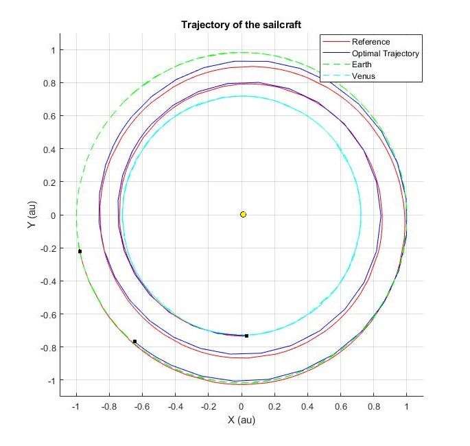
6.1 Outbound Trajectory to 103P/Hartley 2 . . . . . . . . . . . . . . . . . . . . . . . . . . 53
6.2 Sample Return Trajectory to 103P/Hartley 2 . . . . . . . . . . . . . . . . . . . . . . . . 58
7 Conclusions and Recommendations 63
7.1 Conclusions. . . . . . . . . . . . . . . . . . . . . . . . . . . . . . . . . . . . . . . . . . 63
7.2 Recommendations . . . . . . . . . . . . . . . . . . . . . . . . . . . . . . . . . . . . . . 64
A Optimization of three-dimensional solar sailcraft trajectory 67
B Trajectory to 103P/Hartley 2 using a High Performance Sail 69
C Two-dimensional Grid Search Results for the Outbound Trajectory 71
Bibliography 73L IST OF A BBREVIATIONS
AU Astronomical Unit
CCRSR Comet Coma Rendezvous Sample Return
CPU Central Processing Unit
CSSR Comet Surface Sample Return Mission
DE Differential Evolution
DLR Deutsches Zentrum für Luft- und Raumfahrt
EA Evolutionary Algorithm
ESA European Space Agency
GA Genetic Algorithm
GNC Guidance, Navigation and Control
GTOM Global Trajectory Optimization Method
HIF Heliocentric Inertial Frame
IKAROS Interplanetary Kite-craft Accelerated by Radiation of the Sun
JAXA Japan Aerospace Exploration Agency
JPL Jet Propulsion Laboratory
LPE Lagrange Planetary Equations
LTOM Local Trajectory Optimization Method
MEE Modified Equinoctial Elements
NAIF Navigation and Ancillary Information Facility
NASA National Aeronautics and Space Administration
NEA Near-Earth Asteroid
NLP Nonlinear Programming
PAGMO Parallel Global Multiobjective Optimizer
PSO Particle Swarm Optimization
RK Runge-Kutta
RK87DP Variable Step-size Runge-Kutta 8(7) Dormand-Prince method
SA Simulated Annealing
SOF Spacecraft Orbital Reference Frame
SQP Sequential Quadratic Programming
SRP Solar Radiation Pressure
SSB Solar System Barycenter
TOF Time-of-Flight
TPBVP Two-Point Boundary Value Problem
Tudat TU Delft Astrodynamics Toolbox
ixL IST OF S YMBOLS
L ATIN S YMBOLS
a Semi-major axis [m]
ac Characteristic Acceleration [mm/m2 ]
A Sail Surface Area [m2 ]
B f , Bb Front and back Lambertian coefficients [-]
c Speed of light [m/s]
CR DE Crossover factor [-]
D Number of parameters in the decision vector [-]
e Eccentricity [-]
E Eccentric anomaly [deg]
F ,F i ,F r Force acting on an ideal sail [N]
f R , f S , fW Components of perturbing SRP acceleration [ms−2 ]
F DE Weight factor [-]
G Universal Gravitational Constant [m3 kg−1 s−2 ]
h Integration time step [s]
i Inclination [deg]
J Objective Function [-]
Ls Solar Luminosity [W]
m Mass [kg]
M Mean anomaly [deg]
n Orbital Mean Motion [s−1 ]
n̂ Sail normal vector [-]
n̂ H I F Sail Normal in HIF [-]
n̂ SOF Sail Normal in SOF [-]
NP Population size [-]
p, f , g , h, k, L Modified Equinoctial Elements [-]
pw Solar Wind Pressure [N/m2 ]
P Solar Radiation Pressure [N/m2 ]
Px,g Population of vectors [-]
q Perihelion Distance [m]
Q Apohelion Distance [m]
r Radial distance [m]
~
r Position vector [m]
r p , r sai l Position of perturbing body and sailcraft [m]
R Perturbing potential [J/kg]
R Frame Transformation Matrix [-]
RE Sun-Earth Distance [m]
rˆ, dˆ, ĥ Sailcraft Body Centered Reference Axes [-]
tp Time of Perihelion passage [s]
xixii C ONTENTS t0 Time of departure [s] v Velocity [m/s] v i ,g , u i ,g Mutation and Trial vector [-] vw Solar Wind Speed [m/s] v∞ Hyperbolic excess velocity [m/s] W Energy flux from Sun [W/m2 ] x i ,g Target vector [-] x i , x i +1 Sailcraft state at given timestep [-] X,Y,Z Cartesian Coordinate Axes [-] x, y, z Cartesian Coordinates [m] G REEK S YMBOLS α Sail Cone Angle [deg] β Sail Lightness Number [-] δ Sail Clock Angle [deg] ∆ Finite Difference or Increment [-] η Sail efficiency [-] λ Centerline Angle [-] µ Standard Gravitational Parameter [m3 s−2 ] µ̃ Effective gravitational parameter [m3 s−2 ] ν True anomaly [deg] σ Sail loading [g/m2 ] σS A Sail assembly loading [g/m2 ] τ Time interval between nodes [s] ω Argument of Perigee [deg] Ω Right Ascension of the Ascending Node [deg]
1
                                                                I NTRODUCTION
For centuries, we as mankind have been interested in understanding our origin and answering the
fundamental question about the formation of life on Earth. In this quest to understand the early
Solar System formation, a key attribute is about determining the physical and chemical properties
of the primordial mixture, which contained the building blocks for planets and other bodies in the
Solar System. The problem in deducing the composition of this mixture is that over the last 4.5 bil-
lion years since their formation, the planets and their moons have undergone further processing [1].
As a consequence of changes inflicted by high speed impacts between the bodies and due to grav-
itational compression and internal heating, the surface composition of these bodies have evolved
over time and thus, do not offer much insight about early Solar System.

However, some of the other bodies like comets and asteroids, which are considered to have been
formed earlier than the planets, have remained essentially unchanged since their accretion [2].
Comets, especially, orbiting near the outer edges of the Solar System - far from the heat and radia-
tion of the Sun, have remained almost unaltered. Only occasionally, few of the comets pass through
the inner Solar System pulled by gravity, which is witnessed on Earth as the flashy trails across the
night sky. Due to their long orbital periods and minimal interaction with Sun, the chemistry of the
comets has been preserved over time. Thus, comets are considered as the pristine examples of mat-
ter formed from the ancient Solar nebula.

Studying and investigating cometary material could provide information about the primordial mix-
ture from which the planets formed. Such an investigation will also shed some light on cometary
nuclei, exploring the chemistry and physics behind the comet’s activity. Our current knowledge on
comets has been gained through a combination of surface observations and missions to comets.
The presence of ice, ammonia and more importantly, organic compounds like methane and the
amino acid glycine in comets have been confirmed by the past missions to these bodies [3]. These
findings strengthen the theory that water and life on Earth might have been seeded by comets im-
pacting the newly formed Earth. Hence, exploring comets can help in improving our understanding
of planet formation and the origin of life on Earth.

To this end, a science mission to study these bodies is imperative. Though the past flyby or orbiter
missions to comets have provided crucial observations regarding the comet’s physical and chem-
ical characteristics, the scientific benefits of bringing samples of cometary material back to Earth
are far superior. A sample return mission would provide an unique perspective by enabling the
examination of the material returned from the comet in well equipped laboratories [4]. Using the
plethora of instruments and measuring techniques available on ground, higher levels of precision

                                                 1
2 1. I NTRODUCTION can be obtained and the methods can be updated as the technology evolves. This is in contrast to orbiter/lander missions taking in-situ measurements at the comet, which are limited by the number and capability of instruments carried on board the spacecraft. While for a sample return mission, the only specialized equipment needed on board is a simple sample collection and storage device. Additionally, the results inferred from analyzing the returned samples could enhance the value of orbiter/lander observations by validating their findings [4]. The scientific implications of comet sample return missions have made them a prime candidate in Solar System exploration roadmaps of space agencies [5]. Thus, it is essential to analyze the prospect of performing such a mission in the near future. The orbits of comets are, however, challenging to reach due to their high inclination and high eccentricity. Missions to these high energy orbits re- quire a huge amount of ∆V. For conventional propulsion methods which traditionally operate by converting the chemical energy stored in molecules to kinetic energy, this translates to carrying large quantities of propellant on board the spacecraft. As an example, the Rosetta mission (which is just a one-way mission) to comet 67P/Churyumov-Gerasimenko required close to 60% of the or- biter mass as propellant to deliver a payload of 265 kg [6]. This is a major limitation in employing conventional propulsion techniques for comet sample return missions. To overcome this limitation, novel propulsion technique known as solar sailing, is considered for the comet sample return mission in this research. In solar sailing, a large, lightweight sail is used for reflecting the incident radiation from the Sun. The unique advantage of solar sailing is that by using the Sun as the energy source, it does not require propellants as conventional propulsion methods. It is based on the principle of momentum transferred during the impact of a stream of photons (trav- elling at speed of light) onto the sail and thus, the sailcraft [7]. Though, the propulsive force resulting from the momentum transfer to the sail is in the order of few mN, in the frictionless environment of space, this constant energy input can build up to significant proportions over time, enabling the sailcraft to reach great distances in the Solar System. Thus, solar sailing has been considered over the years to possess the potential for interplanetary orbit transfers. The main issues to consider in applying solar sailing is that, firstly, the thrust magnitude decreases as the square of the distance from the Sun. Secondly, unlike other low thrust propulsion systems, the direction of thrust cannot take up any arbitrary vector alignment and is limited by the orientation of the sail. Further since the acceleration attained from solar sailing is very small, the time-of-flight (including the return leg) becomes crucial in accomplishing the mission as well as to prevent the degradation of the sail and other components. In view of the above factors, the trajectory of the so- lar sailcraft needs to be optimized to complete the sample return mission within a reasonable time period. Therefore, the research presented in this thesis report will focus on studying the dynami- cal aspects of the solar sailcraft trajectory to (and back from) the comet. The comet sample return mission will be considered as a time-optimal problem with orbital constraints and the optimal tra- jectory will be determined by employing an optimization algorithm (differential evolution). The outcome of the research will aim to provide more insight into dynamics of the problem, assess the results based on current sailcraft performance level and ultimately, answer the following research question: Is it possible to effectively return cometary samples back to Earth using solar sailing within a reason- able time frame? In order to address the above question, the report begins with the background information on past missions and moves onto discuss mission critical details like target selection and orbital require-
3

ments in Chapter 2. This is followed by Chapter 3, which lays the theoretical foundation of work
done in this thesis, by presenting the choices made regarding the dynamics model used in the sim-
ulation. To determine the optimal trajectory, a number of numerical tools were utilized. Chapter 4
explains the choice of the tools and describes their operation, while Chapter 5 elaborates the pro-
cess of tuning the parameters of these tools and validating their settings. The results of optimization
of the solar sailcraft trajectory for a comet sample return mission are provided in Chapter 6. Finally,
the conclusions derived from this thesis work, along with the recommendations for future research
are presented in Chapter 7.
2
                                                                      B ACKGROUND
The current chapter is used to provide the necessary background to the research topic dealt in this
thesis report. The chapter begins with the history of solar sailing and proceeds to present its ad-
vancement over the years. The various solar sailing missions attempted over the years are briefly
described, along with the breakthrough mission - IKAROS. The presentation of this heritage will
provide the current level of solar sail performance.

A description of the past missions to comets is provided in Section 2.2. The information gained
from these missions was used to decide critical design aspects of the sample return mission. Based
on the design considerations, the mission objectives and the trajectory requirements were derived
and mentioned in Section 2.3. Finally, the possible targets for the comet sample return mission are
listed in Section 2.4 and the choice of the target is also explained.

2.1. H ERITAGE OF S OLAR S AILING
Solar sailing is a novel idea of utilizing the naturally available radiation from the Sun for spacecraft
propulsion. The propulsive force, in case of solar sailing, is obtained through the momentum gained
from the impact of photons on the sail. Though the force resulting from the momentum exchange is
small, the sailcraft is slowly and continuously accelerated, making solar sailing a form of very-low-
thrust propulsion.

The concept of solar sailing as a practical means of spacecraft propulsion was conceived as early as
1924 by the German engineer Fridrickh Tsander [7]. Following this, there were brief studies in the
1950s discussing the advantages of using solar sailing for interplanetary travel. But it was not until
1976 when solar sailing was formally considered for a rendezvous mission to comet Halley by the
National Aeronautics and Space Administration (NASA).

The initial proposal consisted of a 800 x 800 m three-axis stabilized square solar sail [7]. However,
the design was changed to a heliogyro (rotating) configuration with twelve 7.5 km long blades, owing
to the high risk associated with the deployment of the large square sail. Following the preliminary
concept analysis phase, the competing concept of Solar Electric Propulsion (SEP) was selected by
NASA upon its merit of having lower risks for the mission. Ultimately, due to the rising cost estimate,
the comet rendezvous mission was dropped. The analysis and design developments achieved dur-
ing this period sparked the interest in manufacturing and testing key technologies related to solar
sailing for future projects.

                                                   5
6 2. B ACKGROUND
Figure 2.1: Solar Sail deployment test on ground at DLR [9].
In 1999, the Deutsches Zentrum für Luft- und Raumfahrt (DLR) in a joint effort with the European
Space Agency (ESA) successfully tested the first full-scale deployment of a solar sail on ground at
their centre in Cologne. A picture of the deployed sail is given in Figure 2.1. The 20x20 m sail con-
sisted of four segments made of Kapton having a thickness of 7.5 µm, and the sail segments were
deployed with the help of ultra-light weight carbon fiber reinforced plastic (CFRP) booms [8].
Apart from national space agencies, solar sailing also attracted interest from organizations like the
Planetary Society and Cosmos Studios, to set up a private project to test suborbital prototypes.
In 2005, the Cosmos 1 sailcraft (outcome of the collaborative project) marked the first attempt in
demonstrating the solar sail technology on orbit. The 600 m2 sail was made of 5 µm thick alu-
minised reinforced mylar [10]. But due to the malfunctioning of the Volna launcher, the sailcraft
was lost in an explosion just 82 seconds after launch.
Following the above attempts on testing solar sailing technology, the first spacecraft to successfully
demonstrate solar sailing as the main propulsion system in interplanetary space was the Interplan-
etary Kite-craft Accelerated by Radiation Of the Sun (IKAROS), developed by the Japan Aerospace
Exploration Agency (JAXA). The spacecraft comprised of a 14x14 m square sail with a thickness of
7.5 µm [11]. The sail was made of thermoplastic polyimide and had 0.5 kg tip masses at the corners
for stability. Further, thin-film solar cells were embedded on the sail, generating a power of 300 W
and the blocks of LCD (Liquid Crystal Display) panels attached along the edges were used to control
the sail attitude.
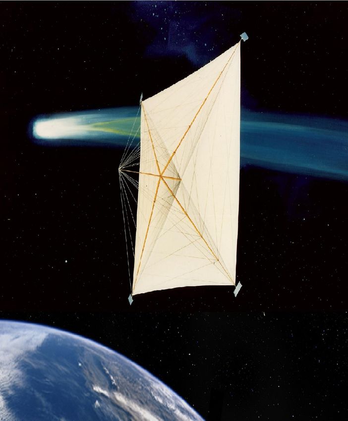
IKAROS was launched aboard the H-IIA rocket from Tanegashima Space Center on 21 May 2010
[11]. With the sail successfully deployed in June 2010, the sailcraft was set on an interplanetary tra-
jectory to Venus. Figure 2.2 shows the picture of IKAROS taken using a Deployable Camera (DCAM)
after sail deployment. During the course of the sailcraft’s trajectory, thrust (and the resulting accel-
eration) due to SRP and the performance of sail’s attitude control system were measured. IKAROS2.1. H ERITAGE OF S OLAR S AILING 7
Figure 2.2: IKAROS in interplanetary space after sail deployment [12].
accomplished its primary goals of deploying the sail, measuring acceleration (and velocity) gained
from SRP and controlling the orientation of the sail. In addition, IKAROS also completed its sci-
entific objectives of detecting and measuring gamma-ray bursts and cosmic dust. Thus, IKAROS
proved to be a landmark in the advancement of solar sail technology and a precursor for making
solar sailing a promising option for space exploration.
With the success of IKAROS, the utilization of solar sailing in space missions increased and ex-
panded to a multitude of applications. NASA’s NanoSail-D2 sailcraft (launched in November 2010)
[13], following a successful sail deployment, remained in the Low Earth Orbit (LEO) for 240 days and
produced large amounts of data on the use of solar sails as passive ways of de-orbiting space debris
and dead satellites. NASA had also planned a solar sailing demonstrator mission called Sunjammer
in 2013 to test sail deployment and sail attitude control, while guiding the sailcraft to the Earth-
Sun L1 Lagrange point. The sail was made of Kapton, having a surface area of 1200 m2 , making it
the largest solar sail built till date [14]. With a large surface area and a thickness of just 5 µm, the
sail was capable of producing thrust in the order of 10−2 N. In spite of Sunjammer being cancelled
before its launch, the design and deployment tests (on ground) were valuable for the research on
manufacture and control of large solar sails.
The Planetary Society after their attempt in 2005 with Cosmos 1, re-initiated their plans with the
LightSail series of sailcraft. The new design was based on NanoSail-D, consisting of a 32 m2 Mylar
sail stacked in a 3U CubeSat format [15]. LightSail-1 was launched as a test mission in May 2015 and
was declared a success following the sail deployment on 7 June 2015. The main mission, LightSail-2,
is scheduled for launch in 2019 and will aim to demonstrate controlled raising of orbit apogee using
solar sail as main propulsion.
In view of the results achieved and progress made in solar sailing technology, more missions have
been planned for the forthcoming future. Among the recently proposed missions is the ESA/DLR
collaborative project - Gossamer Roadmap - which would send series of demonstrator sailcraft
called Gossamer-1,-2 and -3 to space [16]. The objective of the project is to demonstrate the de-
ployment and full attitude and orbit control of 5x5 m, 10x10 m and 50x50 m sails, that can be used
to deorbit small satellites from LEO. Another important mission is NASA’s Near Earth Asteroid (NEA)
Scout mission, which will demonstrate the ability of low-cost sailcraft to perform NEAs reconnais-8 2. B ACKGROUND
sance. The sailcraft will be in a 6U cubesat formation, weighing just 12 kg and propelled by a 83
m2 sail [17]. Notably, NEA Scout will be one of several payloads aboard the maiden flight of NASA’s
Space Launch System (SLS), scheduled to be launched in 2019.
Finally, OKEANOS (Outsized Kite-craft for Exploration and Astronautics in the Outer Solar System)
is a proposed solar sail mission by JAXA to Jupiter’s Trojan asteroids [18]. The spacecraft will be
propelled by a hybrid solar sail, containing thin solar panels embedded on the sail to power an ion
engine. As a supplementary part of the mission, lander and sample return options are considered
and if selected, the mission will be launched in late 2020s.
From the time when solar sailing was considered a concept for novels, it has made giant strides
in becoming a reality, through the efforts of scientists and engineers over the years. Especially in
the last decade, missions like IKAROS and NanoSail-D2 have demonstrated the capabilities and
the wide range of applications that the technology possesses, some of which are unique to solar
sailing. The current research focuses on further reducing the mass per unit area of the sail (called
the sail loading parameter), to enable ambitious mission concepts to outer Solar System or to place
satellites in non-Keplerian orbits. Additionally, performing further flight tests on sail deployment
and attitude control would make the technology more robust and reliable. Therefore, with the rising
opportunities for solar sailing and future advancements in place, solar sailing has the potential to
become a viable option for space exploration.
2.2. M ISSIONS TO C OMETS
Comets are small bodies made of ice and dust, and are known to originate from the outer regions of
the Solar System. The core of the comets called the nucleus consists of a combination of dust, rock,
ice and frozen oxides of carbon [20]. Due to the heat from solar radiation, the ice and frozen ox-
ides sublimate from the nucleus forming a thin atmosphere called the coma. The presence of these
gases and ions in the coma is responsible for the comet’s brightness, which lead to the detection of
numerous comets. During the comet’s passage close to the Sun, the force exerted by solar wind on
the coma creates a plasma tail pointing away from the Sun. The sublimation of ice from the nucleus
drags along the dust particles as the gases release from the surface, forming an additional dust tail
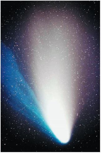
(shaped by solar radiation pressure) as depicted in Figure 2.3. These tails can be generally observed
Figure 2.3: Depiction of the plasma (blue) and dust (white) tails of a comet [19].2.2. M ISSIONS TO C OMETS 9 to extend to great lengths (in the order of 107 km) from the comet, but the density of particles re- duces rapidly with the distance from the comet. The comets, along with the planets and asteroids, are considered to have been formed from the collapse of a dense, molecular cloud made of dust, gas and ice [21]. However, the planets have all been subjected to significant reprocessing since their formation and do not provide much infor- mation about the material from which they formed. Whereas, comets having spent only a small fraction of their orbital period in the inner Solar System, remain pristine, free from reprocessing of their material or structure. The comets are also considered to be of high astrobiological value due to the possibility that comets might have contributed to the presence of life and volatile compounds found on Earth [22]. Thus, observing and exploring comets has been one of the important priorities for the space agencies around the world, to further the understanding of the solar System. In the past, there have been space missions to study the comets at a close range, including flyby, rendezvous, orbiter or sample return missions. Amongst the previous missions to comets, Deep Impact, Rosetta and Stardust were unique and their observations were pivotal for the current knowl- edge about these bodies. In the Deep Impact mission, NASA released an impactor into the comet, to study the interior composition of the comet 9P/Tempel by observing the collision. The spacecraft was launched on a Delta-II rocket from Cape Canaveral on January 12, 2005 [23]. Following the 60 days cruise phase, the spacecraft began its approach towards the comet, while also observing the comet’s position, activity, rotation and dust environment. The 372 kg impactor was detached from the flyby spacecraft on June 29, 2005 and was positioned in front of the comet for an impact on July 4, 2005. The Deep Impact spacecraft took images of the event and its outcome from a safe distance of about 500 km from the comet. The crater formed due to the impact was measured to be around 150 m in diameter and 30 m in depth [24]. The image analysis of the impact revealed that the material ejected consisted of more dust particles (finer than sand) and fewer ice than presumed. More detailed in- formation could not be recognized from the images due to the bright dust cloud over the crater. Another mission named Stardust was used as a follow-up to obtain better images of the crater. The data from these missions indicated the presence of materials containing carbon as well as water ice on the comet 9P/Tempel 1 [24]. Based on the results, Tempel 1 was envisaged to have originated in the Uranus and Neptune Oort Cloud region of the Solar System. The Deep Impact mission was ex- tended to observe other comets including 103P/Hartley 2, before ending the mission in September 2013. The observations made at the Hartley 2 revealed a crucial detail that the comet was made of dry ice and not water ice as anticipated earlier. ESA’s Rosetta mission features as an important milestone in the study of comets and for demon- strating the technological advancement achieved in the field of space exploration. The objective of the mission was to orbit comet 67P/Churyumov Gerasimenko and conduct an extensive investiga- tion of the comet [6]. Towards this aim, the spacecraft was designed to consist of two parts, viz., an orbiter and a lander (Philae). The orbiter was used to observe the comet’s activities and the lander was employed to make in-situ measurements of it’s composition. On March 2, 2004, the spacecraft was launched on an Ariane 5 rocket from the Guiana Space Centre [6]. The main propulsion system of the spacecraft consisted of 24 paired bipropellant (monomethylhydrazine-dinitrogen tetroxide) 10 N thrusters, which were used for orbit maneuvers and attitude control. Rosetta’s trajectory to the comet included gravity assist maneuvers and flybys, with the first Earth flyby on March 4, 2005 [26]. To correct its trajectory, the spacecraft made a low-altitude flyby of Mars in February 2007, which was followed by two more Earth flybys in November 2007 and November 2009 respectively. After
10                                                                                     2. B ACKGROUND

Figure 2.4: Illustration of the trajectory followed by Rosetta to Comet 67P/Churyumov-Gerashimenko [25].

ten years long journey, Rosetta entered into the orbit around the comet on August 6, 2014, after per-
forming a series of rendezvous maneuvers.

Immediately after getting into the orbit around the comet, the orbiter surveyed the comet’s surface
for potential sites for deploying the lander. On November 12, 2014, the Philae lander detached from
the orbiter and landed on the comet [26]. After a brief hiatus, the lander completed most of planned
measurements and transmitted the obtained data back to Earth via the orbiter. Due to the decrease
in sunlight received by the spacecraft as the comet travelled through the outer Solar System and as
the communication with the orbiter/lander did not look optimistic, the mission was concluded by
guiding the orbiter to the comet’s surface. Being a recent mission, interpretation of data sent by the
spacecraft are still ongoing. From the initial analysis, the isotopic signature of water vapour on the
comet was found to be different to that on Earth [28]. The measurements made by Philae indicate
the presence of carbon and hydrogen molecules in the coma. Further, the material displaced at
Philae’s landing site revealed traces of organic compounds, few of which were observed for the first
time on a comet.

Till date, Stardust is the first and only mission to have achieved the feat of bringing back samples
from the coma of a comet back to Earth. In 1995, NASA set up Stardust as a dedicated mission to

                          Figure 2.5: Illustration of the Stardust spacecraft [27].
2.2. M ISSIONS TO C OMETS 11
Figure 2.6: Stardust mission trajectory [27].
study Comet Wild 2, a long-period comet believed to hold pristine samples of materials from its
formation. The spacecraft was launched aboard a Delta-II rocket from Cape Canaveral on February
7, 1999 [29]. The main objective of the mission was to make a non-destructive capture of particles
from the comet’s coma and return the samples safely back to Earth. The spacecraft followed a he-
liocentric orbit (Figure 2.6) that took it around the Sun and approached the Earth for a gravity assist
maneuver in 2001. After around 5 years en route to the comet, Stardust performs a close flyby at a
distance of 240 km to the comet, with the sample collector deployed to collect particles.
To prevent damage during particle collection, the sample collector was designed in the shape of a
tennis racket as shown in Figure 2.5, containing blocks of ultra-low density aerogel in silicon-based
porous structures [29]. Five other scientific payloads (Imaging Camera, Dust Flux Monitor, Dust
Analyzer, Sample Collection Instrument and Telecommunication Unit) were carried on-board to
capture images of the comet and perform real-time analysis to determine the composition, mass
and size of the collected dust particles. On January 15, 2006 after around two years on its return
trajectory, Stardust reached Earth and released the Sample Return Capsule, which re-entered the
Earth’s atmosphere and landed safely in the Utah desert.
The comet’s samples were examined in the clean room at NASA’s Johnson Space Center in Houston.
More than a million microscopic dust particles were embedded in the aerogel, along with few parti-
cles in the size range of 0.1 mm [30]. The preliminary analysis of the samples indicated the presence
of a large number of organic compounds, with some of the compounds containing biologically us-
able nitrogen. The existence of iron and copper sulfide in the samples suggested the heating of
comet’s core during the early Solar System, since the formation of these molecules require the pres-
ence of water [31]. Additionally, for the first time, glycine (an amino acid) was detected in the parti-
cles ejected from Wild 2, supporting the theory that life in the Universe could be common and not
rare.12 2. B ACKGROUND 2.3. M ISSION O BJECTIVES The current knowledge on comets is based on the information gained from optical remote sens- ing, computer simulations, study of meteoritic materials found on Earth, flyby missions to comets and examination of samples returned from Comet Wild 2 [21]. The space missions, especially, were crucial for expanding our understanding of the comets as well as for verifying some of the existing theories on comets. The samples retrieved by Stardust spacecraft appears to be composed of a het- erogeneous mixture of organics and minerals. Intermingled in these mixtures, a collection of highly refractory and highly volatile components were also found. Few of these components show clear isotopic evidence of pre-solar materials [21]. Thus, the study on cometary samples has successfully shown that comets possess materials originating from a wide range of environments, making them a repository of primordial Solar System materials. Although the samples brought back by Stardust were vital in arriving at the above insights, the parti- cle collection had its drawback as well. The particles from comet Wild 2’s coma was collected in the aerogel collector at a relative velocity of around 6.1 km/s with respect to the comet [21]. Due to this high impact velocity, only some of the particles survived unaltered, while others were either altered or destroyed. This in turn affects the interpretation of particle characteristics and determination of their elemental composition, as there is a possibility for some components to be selectively altered or lost over others. Hence, these samples do not yet provide answers to some of the key questions regarding - (i) the presence of volatile organics and nebular condensate amorphous silicates, (ii) relative concentration of minerals/organics, and (iii) the radiometric chronology of comets and the early Solar System [21]. Based on the lessons learnt from the Stardust mission, certain points for improved results were suggested in the concept study on Comet Coma Rendezvous Sample Return mission (CCRSR) [21]. Primarily, as the Stardust spacecraft returned with less than 1000 particles with size greater than 15 µm, it would be beneficial for statistical analysis if close to hundred times more particles were col- lected by flying closer to the comet and/or allowing longer collection times. Such an increase in the sample size of particles collected will enhance the chance of identifying the particle types, finding particular organic molecules, collecting rare minerals and establishing the isotopic chronologies of the materials. It was also suggested that the particles should be collected using high-purity metallic meshes, in order to avoid organic contaminants, extraneous materials and the ubiquitous compo- nents (Si and O) of the aerogel. Secondly, the study also recommended that the samples need to be collected at relative velocities less than 0.1 km/s, so that the particles do not suffer any alteration during collection, thus yield- ing unbiased, pristine samples of the cometary material [21]. Apart from the constraints placed on sample collection, the overall time period of the mission - from launch till return of samples to Earth - needs to be set. The mission duration is one of the driving factors which influences the reliability requirements of various spacecraft subsystems. Obviously, the longer is the mission, the more reli- able, withstanding and long lasting should be components, which is extremely challenging due to the harsh environment in space. In a comet sample return concept study by NASA [32], a maximum time limit of 10 years was set for the overall mission duration considering the safety of the samples as well during the transit. Further, since in this thesis, solar sailing will be used as the main propulsion, the degradation of the sail material from constant exposure to solar radiation should be considered as well when deciding the mission duration. In this regard, the study on Near-Earth Asteroid (NEA) sample return using solar sailcraft [33] also employed a 10 year time period for maximum mission duration. Due to the similar nature of the missions in the above mentioned concept studies and the
2.4. M ISSION TARGET                                                                                     13

one considered in this thesis, the total mission duration was constrained to be within 10 years.

Based on the discussion on past missions and sample return mission concept studies, the following
scientific outcomes are expected as a result of the solar sailcraft comet sample return mission:

    • To determine the relative concentrations of minerals and organics.

    • To establish a radiometric chronology for comets.

    • To check for materials of interstellar origin (like amorphous silicate condensate).

    • To understand the nature of evolution and extinction of cometary ice.

    • To check for the presence of simple biomolecules.

To achieve the above objectives, certain requirements are placed on the sailcraft trajectory for the
mission considered in this thesis. These are:

    • The sailcraft shall collect samples from the comet’s coma at a distance less than 250 km.

    • Sample collection shall take place at a relative velocity of less than 0.1 km/s with respect to
      the comet.

    • The overall mission duration shall be less than 10 years.

    • For effective sample collection, the sailcraft shall collect the samples during the comet’s peri-
      helion passage.

2.4. M ISSION TARGET
Comets have been observed by mankind for many centuries but it was not until 1759 that a comet’s
orbital characteristics were studied and catalogued. This was done for the first time for the comet
1P/Halley. Following that, numerous comets have been identified and added to the catalogue.
Presently, over 5882 comets have been identified, with around 3958 comets having an official desig-
nation [34].

Given such an extensive list of comets, it is challenging to narrow it down to a comet as the target for
our comet sample return mission. Hence, few selection criteria were established to filter through the
number of comets suitable for the mission. Possible mission targets are short-listed based on the
scientific interest to study the comet, and the practical viability of reaching the comet and returning
samples to Earth. Since, solar sailing trajectory evolves slowly, the target’s perihelion distance is
desired to be within 0.5 AU from the Earth’s orbit and considering the overall mission duration, the
target comet’s orbit shall be close to the ecliptic plane. The list of criteria used to filter the potential
targets for the mission are:

    • Comets perihelion distance (q) should be close to Earth’s orbit (≤0.5 AU).

    • Comets’ orbit should be prograde and close to the ecliptic plane (i < 20◦ )

    • Comets next perihelion passage must occur within 2020 and 2030, to have a realistic launch
      window.

    • Comets whose basic physical characteristics like size, mass and shape have already been stud-
      ied are preferred, to minimize the mission risk.
14 2. B ACKGROUND The final condition on the list is to prevent designing a mission to a target whose physical and or- bital parameters are not yet known accurately due to very few observational sitings. However, at the same time, comets that have been studied extensively in the past like the Halley’s comet are also not preferred for the mission, in order to avoid redundancy and explore new frontiers. Based on NASA’s list of priority comet targets of high scientific importance [35] and targets short- listed in the concept study for the Comet Surface Sample Return (CSSR) mission [32], a list of poten- tial targets was obtained as shown in Table 2.1. The data on the comet’s orbit were taken from JPL’s Small Bodies Database [34]. Table 2.1: Potential targets for comet sample return mission using a solar sailcraft (data obtained from [34]). Comet e q (AU) i (deg) ω (deg) Ω (deg) Q (AU) Period (yrs) Classification 2P/Encke 0.8483 0.3360 11.7801 186.5420 334.5686 4.0942 3.30 NEO 6P/d"Arrest 0.6114 1.3615 19.4810 178.1152 138.9337 5.6459 6.56 Jupiter-family 8P/Tuttle 0.8198 1.0271 54.9832 207.5092 270.3417 10.3726 13.61 Jupiter-family (NEO) 9P/Tempel 1 0.5175 1.5066 10.5305 178.8771 68.9334 4.7383 5.52 Jupiter-family 15P/Finlay 0.7205 0.9746 6.8036 347.5656 347.5656 13.8006 6.51 Jupiter-family (NEO) 19P/Borrelly 0.6232 1.3598 30.3130 353.3507 75.4359 5.8595 6.86 Jupiter-family 21P/Giacobini-Zinner 0.7068 1.0307 31.9081 172.5844 195.3970 6.0004 6.59 Jupiter-family (NEO) 41P/Tuttle–Giacobini–Kresák 0.6612 1.0450 9.2293 62.1566 141.0677 5.1248 5.42 Jupiter-family (NEO) 55P/Tempel-Tuttle 0.9055 0.9764 162.4865 172.5003 235.2701 19.7002 33.24 Halley-type (NEO) 67P/Churyumov-Gerasimenko 0.6406 1.2453 7.0437 12.6944 50.1800 5.6842 6.45 Jupiter-family 79P/du Toit-Hartley 0.6185 1.1238 3.1456 281.6893 280.6403 4.7679 5.06 Jupiter-family (NEO) 81P/Wild 2 0.5370 1.5979 3.2372 41.7596 136.0977 5.3060 6.41 Jupiter-family 103P/Hartley 2 0.6938 1.0642 13.6043 181.3223 219.7487 5.8863 6.48 Jupiter-family (NEO) Out of the 13 potential targets, four comets (8P, 19P, 21P and 55P) have inclination greater than the specified criterion of 20◦ and another four comets (2P, 9P, 6P and 81P) do not have their perihelion distance close to the Earth’s orbit. Among the remaining comets, only comets 67P and 103P have been visited by spacecraft previously. However, comet 67P/Churyumov-Gerasimenko was the target of the recently concluded Rosetta mission, during which the comet was studied in detail using a combination of orbiter and lander. Whereas, comet 103P/Hartley 2 was briefly observed by the Deep Impact spacecraft as part of its extended mission. Using the data from Deep Impact mission, the comet’s physical properties were determined. But, being a flyby mission, the comet was not studied comprehensively, making it an ideal target for a sample return mission. A follow-up sample return mission could (i) provide better insight about the comet’s composition, (ii) confirm the existing observational data, and (iii) obtain chronological information regarding its origin and evolution. Therefore, the comet 103P/Hartley 2 was selected as the target for the comet sample return mission using a solar sailcraft.
3
                                                                                   T HEORY
This chapter lays the foundation of the theoretical concepts used in this thesis for simulating the
sailcraft trajectory. First, the basic astrodynamic concepts of reference frames and coordinate sys-
tems are introduced. This is followed by a discussion on the forces and dynamics model considered
to describe the motion of the solar sailcraft. In Section 3.5, the principles and dynamics of solar
sailing are explained, along with the sail design parameters. Finally, the equations of motion repre-
senting the sailcraft’s trajectory are presented in Section 3.6.

3.1. R EFERENCE F RAMES
In astrodynamics, to describe/simulate the motion of a spacecraft, it is vital to know (at least) the
position and mass of the celestial bodies involved. As position and velocity are relative quantities,
they are defined with respect to a reference system. The reference system completely describes the
formation of a celestial coordinate system, in terms of origin and orientation of fundamental planes
and axes [36]. Using a reference system, any point in space can be specified by a unique set of coor-
dinates.

From Newtonian mechanics, two classes of reference frames can be defined [36]. Reference frames
which are at rest or moving at constant velocity in a straight line are considered as inertial refer-
ence frames. Whereas, non-inertial reference frames are either in a rotational or accelerated mo-
tion. Newton’s laws of motion are valid only in inertial reference frames, while apparent (or pseudo)
forces have to be included when applying Newtonian mechanics in non-inertial reference frames.

There are applications that demand motion to be described about a rotating or accelerating body.
For example, specifying the location of a launch site on the surface of Earth or the orientation of an
instrument with respect to the satellite. In such cases, non-inertial reference frames are considered
along with their associated pseudo forces like centrifugal, Coriolis or Euler forces [36]. Therefore,
with the help of the above force models, a transformation matrix can be defined to convert between
inertial and non-inertial frames.

As no additional force terms are required in inertial reference frames, the mathematical complexity
of equations describing the motion of a body are significantly reduced. Hence, these frames are
preferred for representing the motion of spacecraft, in orbit around a body or on a transfer trajectory
to a target. In this section, the reference frames which were used in this thesis work, to describe the
orbital dynamics and to model the sail force, are discussed.

                                                  15
16 3. T HEORY
Figure 3.1: Heliocentric Reference Frame [37].
3.1.1. H ELIOCENTRIC R EFERENCE F RAME
Heliocentric reference frames are centered at the Sun or at the barycenter (center of mass) of the
Solar System. As the bodies in the Solar System revolve around the Sun, these frames are commonly
used for describing interplanetary trajectories. Although the Sun itself is orbiting the center of the
Milky Way galaxy, considering the time scale of the rotation and the influence of Sun’s gravitational
field within the Solar System, the origin of the heliocentric reference frame can be considered to be
fixed.
The fundamental plane of the heliocentric reference frame is taken to be Earth’s orbital plane (eclip-
tic) around the Sun, since the orbits of other planets have small inclinations with respect to the
ecliptic. The +Z-axis of this frame is along the ecliptic north pole direction, with the +X-axis lying in
the ecliptic plane and pointing towards the Vernal equinox (the First point of Aries) [37]. The +Y-axis
completes the right-handed system as given in Figure 3.1. Due to the effect of precession and nuta-
tion, the direction of the Vernal equinox shifts slowly over the centuries with respect to extragalatic
sources like quasars [36]. Therefore, in order to define the reference axes direction, the orientation
of the heliocentric ecliptic reference frame on 1 January 2000 at 12:00 terrestrial time is typically
taken as the reference. The resulting heliocentric ecliptic inertial frame of reference is referred as
ECLIPJ2000.
The ECLIPJ2000 frame is widely used in many astrodynamics tools and software due to its temporal
reference and compatibility. Furthermore, the Solar System ephemeris information system (called
SPICE), maintained by the Navigation and Ancillary Information Facility (NAIF) under NASA’s Plan-
etary Science division, is available in the ECLIPJ2000 frame [38]. This means the ephemeris data
from SPICE can be directly used in the astrodynamic tool (Tudat) for trajectory simulation. The
ECLIPJ2000 reference frame will thus be the fundamental reference frame for simulating the trajec-
tory of the solar sailcraft in this thesis work, due to its inertial, space-fixed nature and availability of
ephemeris data with respect to this frame.
3.1.2. S PACECRAFT ORBITAL REFERENCE FRAME
A spacecraft orbital reference frame has its origin at the center of mass (CM) of the spacecraft. It is
used for describing the relative dynamical motion of various systems or components of a spacecraft3.1. R EFERENCE F RAMES 17
Figure 3.2: Spacecraft orbital reference frame [39].
like solar arrays, antennas or - in case of sailcraft - the sail itself. In solar sailing, the sail orientation
determines both the direction and magnitude of the thrust force resulting from the SRP acting on
the sail. The definition of the spacecraft reference frame thus plays a important role in expressing
the orientation of the sail.
The axes of the frame are defined based on three unit vectors as shown in Figure 3.2. The radial unit
vector rˆ points in the direction of the Sun-sail line, unit vector ĥ points along the sailcraft’s orbital
angular momentum vector and finally, the transversal unit vector dˆ completes the right-handed ref-
erence frame [39]. The velocity vector (v) of the sailcraft, therefore, lies in the plane formed by unit
vectors rˆ and dˆ.
As the frame is centered at the CM of the spacecraft, it rotates as the spacecraft moves in its orbit
around the Sun. Thus, the frame is non-inertial and if equations of motion were to be solved in this
frame apparent forces should be included. To avoid this complication, the sail orientation is trans-
formed from the spacecraft reference frame to the heliocentric reference frame and the equations
are solved in the heliocentric frame.
3.1.3. R EFERENCE F RAME T RANSFORMATION
From the previous subsections, it can be seen that two reference frames are to be used to describe
the motion of the sailcraft. The ECLIPJ2000 frame is utilized for specifying the position and velocity
of the sailcraft with respect to the Solar System barycenter (SSB). While the spacecraft orbital ref-
erence frame (SOF) is used for representing the sail attitude and calculating the acceleration due
to SRP. Therefore, the sail normal vector in SOF needs to be transferred to the ECLIPJ2000 for force
calculation and trajectory propagation, at every integration timestep.
n SOF ) is defined as
The sail normal vector in SOF (~
cos α
~
n SOF = sin α sin δ (3.1)
sin α cos δ
where α and δ are the cone and clock angles respectively that unequivocally define the sail attitude
in SOF. The cone angle α is defined as the angle between the sail normal vector (n̂) and Sun-sail line
(rˆ) in radial direction [7]. Whereas the clock angle δ is measured between the transverse unit vector
(dˆ) and the projection of n̂ on the plane perpendicular to the Sun-sail line as depicted in Figure 3.3.18 3. T HEORY
Figure 3.3: Representation of sail cone and clock angles (modified from [40]).
The unit vectors of the three axes of SOF are given by [41]
~
r ~
r ×~
v
rˆ = , ĥ = , dˆ = rˆ × ĥ (3.2)
r|
|~ r ×~
|~ v|
where ~
r and ~
v are the position and velocity vectors of the sailcraft respectively. The frame transfor-
mation matrix R from SOF to ECLIPJ2000 is [41]:
R = rˆ dˆ ĥ
¡ ¢
(3.3)
Thus, the sail normal vector in the heliocentric inertial frame is
n̂ H I F = R n̂ SOF (3.4)
3.2. C OORDINATE S YSTEMS
A coordinate system provides the method for locating a point within the reference frame. The coor-
dinate systems thus play an essential role in expressing the position, velocity or the complete state
of celestial bodies and spacecraft along their trajectory. The coordinate systems used to character-
ize the solar sail trajectories in this thesis work are discussed in this section. Finally, the choice of
the coordinate system which was employed to write the equations of motion is also explained in
Section 3.2.3.
3.2.1. C ARTESIAN C OORDINATES
The Cartesian coordinate system is one of the most commonly used coordinate systems in the fields
of mathematics, science and engineering. The position of a point is specified by three spatial coor-
dinates (x, y, z) which represent the signed distance of its projection on the three frame axes from
the frame origin O. The state of a body in Cartesian coordinates (x, y, z, ẋ, ẏ, ż) is represented as a
combination of position and velocity components [36].You can also read


