Online Caching Networks with Adversarial Guarantees

Online Caching Networks with Adversarial Guarantees
YUANYUAN LI, Northeastern University, USA
TAREQ SI SALEM, Université Côte D’Azur, Inria, France
GIOVANNI NEGLIA, Inria, Université Côte D’Azur, France
STRATIS IOANNIDIS, Northeastern University, USA
We study a cache network under arbitrary adversarial request arrivals. We propose a distributed online policy
based on the online tabular greedy algorithm [77]. Our distributed policy achieves sublinear (1 − 1 )-regret,
also in the case when update costs cannot be neglected. Numerical evaluation over several topologies supports
our theoretical results and demonstrates that our algorithm outperforms state-of-art online cache algorithms.
CCS Concepts: • Information systems → Storage management; • Theory of computation → Online
algorithms; Caching and paging algorithms; Distributed algorithms; Submodular optimization and 35
polymatroids.
Additional Key Words and Phrases: Caching Network, Adversarial Guarantees, Online Optimization, No-Regret
Algorithms
ACM Reference Format:
Yuanyuan Li, Tareq Si Salem, Giovanni Neglia, and Stratis Ioannidis. 2021. Online Caching Networks with
Adversarial Guarantees. Proc. ACM Meas. Anal. Comput. Syst. 5, 3, Article 35 (December 2021), 39 pages.
https://doi.org/10.1145/3491047

1 INTRODUCTION
We study network of caches, represented by an arbitrary topology, in which requests for contents
arrive in an adversarial fashion. Requests follow paths along the network towards designated servers,
that permanently store the requested items, and can be served by caches of finite capacity residing
at intermediate nodes. Responses are carried back over the same path towards the source of each
request, incurring a cost. Our objective is to propose a distributed, online algorithm determining
cache contents in a way that minimizes regret, when both items requested as well as paths they
follow are selected adversarially.
 The offline version of this problem is NP-hard, but admits a (1 − 1/ ) polytime approximation
algorithm [73]. Ioannidis and Yeh [41] proposed a distributed Robbins Monro type algorithm that
attains the same approximation guarantee assuming stochastic, stationary request arrivals. This
model has motivated several variants [35, 43, 54–57, 79], the majority of which focus on offline
and/or stationary stochastic versions of the problem. Another thread of recent research in caching,
spurred by the seminal work of Paschos et al. [66], explores caching algorithms that come with
adversarial guarantees. The majority of these works focus either on a single cache [62, 71, 74] or
on simple, bipartite network topologies [10, 65, 66].
Authors’ addresses: Yuanyuan Li, yuanyuanli@ece.neu.edu, Northeastern University, Boston, USA; Tareq Si Salem, tareq.si-
salem@inria.fr, Université Côte D’Azur, Inria, Sophia Antipolis, France; Giovanni Neglia, giovanni.neglia@inria.fr, Inria,
Université Côte D’Azur, Sophia Antipolis, France; Stratis Ioannidis, ioannidis@ece.neu.edu, Northeastern University, Boston,
USA.

Permission to make digital or hard copies of all or part of this work for personal or classroom use is granted without fee
provided that copies are not made or distributed for profit or commercial advantage and that copies bear this notice and
the full citation on the first page. Copyrights for components of this work owned by others than ACM must be honored.
Abstracting with credit is permitted. To copy otherwise, or republish, to post on servers or to redistribute to lists, requires
prior specific permission and/or a fee. Request permissions from permissions@acm.org.
© 2021 Association for Computing Machinery.
2476-1249/2021/12-ART35 $15.00
https://doi.org/10.1145/3491047

 Proc. ACM Meas. Anal. Comput. Syst., Vol. 5, No. 3, Article 35. Publication date: December 2021.

35:2 Yuanyuan Li et al.

 The main objective of this paper is to bring adversarial guarantees to the general network model
proposed by Ioannidis and Yeh. From a technical standpoint, this requires a significant technical
departure from the no-regret caching settings studied by prior art [10, 62, 65, 66, 71, 74], both due
to its distributed nature and the generality of the network topology. For example, our objective
cannot be optimized directly via techniques from online convex optimization [39, 72, 81] to attain
sublinear regret.
 We make the following contributions:
 • We revisit the general cache network setting of Ioannidis and Yeh [41] from an adversarial
 point of view. √
 • We propose DistributedTGOnline, a distributed, online algorithm that attains ( )
 regret with respect to an offline solution that is within a (1 − 1/ )-approximation from the
 optimal, when cache update costs are not taken into account. √
 • We also extend our algorithm to account for update costs. We show that an ( ) regret
 is still attainable in this setting, replacing however independent caching decisions across
 rounds with coupled ones; we determine the latter by solving an optimal transport problem.
 • Finally, we extensively evaluate the performance of our proposed algorithm against several
 competitors, using (both synthetic and trace-driven) experiments involving non-stationary
 demands.
 The remainder of this paper is organized as follows. In Section 2, we review related work. Our
model and distributed online algorithm are presented in Sections 3 and 4, respectively. We present
our analysis of the regret under update costs in Section 5 and extend our results in Section 6. Our
experiments in Section 7. We conclude in Section 8.

2 RELATED WORK
Content allocation in networks of caches has been explored in the offline setting, presuming demand
is known [12, 68, 73]. In particular, Shanmugam et al. [73] were the first to observe that caching
can be formulated as a submodular maximization problem under matroid constraints and prove its
NP-hardness. Dynamic caching policies have been mostly investigated under a stochastic request
process. One line of work relies on the characteristic time approximation [18, 27, 32, 46, 47] (often
referred to as Che’s approximation) to study existing caching policies [3, 7, 22, 31] and to design
new policies that optimize the performance metric of interest (e.g., the hit ration or the average
delay) [25, 53, 63]. Another line proposes caching policies inspired by Robbins-Monro/stochastic
approximation algorithms [40, 41].
 In particular, Ioannidis and Yeh [42] present (a) a projected gradient ascent (PGA) policy that
attains (1 − 1/ )-approximation guarantee in expectation when requests are stationary and (b)
a practical greedy path replication heuristic (GRD) that performs well in many cases, but comes
without guarantee. Our work inherits all modeling assumptions on network operation and costs
from [42], but differs from it (and all papers mentioned above) by considering requests that arrive
adversarially. In our experiments, we compare our caching policy with PGA and GRD, that have no
guarantees in the adversarial setting. We also prove that GRD in particular has linear regret (see
Lemma 4.3).
 Sleator and Tarjan [75] were the first to study caching under adversarial requests. In order to
evaluate the quality of a caching policy, they introduced the competitive ratio, that is the ratio
between the performance of the caching policy (usually expressed in terms of the miss ratio) and
that of the optimal clairvoyant policy that knows the whole sequence of requests. This problem was
generalized under the name of -server problem [59] and metrical task system [11] and originated
a vast literature (see, e.g., the survey [51]). In this paper, we focus on regret rather than competitive

Proc. ACM Meas. Anal. Comput. Syst., Vol. 5, No. 3, Article 35. Publication date: December 2021.

Online Caching Networks with Adversarial Guarantees 35:3

ratio to quantify the main performance metric. Roughly speaking, the regret corresponds to the
difference between the performance of the caching policy and the optimal clairvoyant policy (see [4]
for a thorough comparison of regret and competitive ratio). The regret metric is more popular in
the online learning literature. The goal is to design algorithms whose regret grows sublinearly with
the time horizon and thus have asymptotically optimal time-average performance.
 To the best of our knowledge, Paschos et al. [66] were the first to apply online learning techniques
to caching. In particular, building on the online convex optimization framework [39, 72, 81], they
propose an online gradient descent caching algorithm with sublinear regret guarantees, both for a
single cache and for a bipartite network where users have access to a set of parallel caches (the
“femtocaching” scenario in [73]) and items are random linearly encoded. Si Salem et al. [74] extend
this work considering the more general family of online mirror descent algorithms [13], but only
considered a single cache. Bhattacharjee et al. [10] prove tighter lower bounds for the regret in the
femtocaching setting and proposed a caching policy based on the Follow-the-Perturbed-Leader
algorithm that achieves near-optimal regret in the single cache setting. These results have been
extended to the femtocaching setting [65]. Two recent papers [62, 71] pursued √ this line of work
taking into account update costs for a single cache. We provide similar ( ( )) regret guarantees
for general cache networks (rather than just bipartite ones), using a different algorithm.
 As mentioned above, content placement at caches can be formulated as a submodular optimization
problem [41, 73]. The offline problem is already NP-hard, but the greedy algorithm achieves 1/2
approximation ratio [30]. Calinescu et al. [15] develop a (1 − 1/ )-approximation through the so
called continuous greedy algorithm. The algorithm finds a maximum of the multilinear extension
of the submodular objective using a Frank-Wolfe like gradient method. The solution is fractional
and needs then to be rounded via pipage [2] or swap rounding [19]. Filmus and Ward [29] obtain
the same approximation ratio without the need of a rounding procedure, by performing a non-
oblivious local search starting from the solution of the usual greedy algorithm. These algorithms
are suited for deterministic objective functions. Hassani et al. [38] study the problem of stochastic
continuous submodular maximization and use stochastic gradient methods to reach a solution
within a factor 1/2 from the optimum. Mokhtari et al. [61] propose then the stochastic continuous
greedy algorithm, which reduces the noise of gradient approximation by leveraging averaging
technique. This algorithm closes the gap between stochastic and deterministic submodular problems
achieving a (1 − 1/ )-approximation ratio.
 There are two kinds of online submodular optimization problems. In the first one, a.k.a. competi-
tive online setting, the elements in the ground set arrive one after the other, a setting considerably
different from ours. The algorithm needs to decide whether to include revealed elements in the
solution without knowing future arrivals. Gupta et al. [34] consider the case when this decision is
irrevocable. They give a (log )-competitive algorithm where is the rank of matroid. Instead,
Hubert Chan et al. [17] allow the algorithm also to remove elements from the current tentative
solution. They propose a randomized 0.3178-competitive algorithm for partition matroids. In the
second kind of online submodular optimization problems, objective functions are initially unknown
and are progressively revealed over rounds. This setting indeed corresponds to our problem,
as our caching policy needs to decide the content allocation before seeing the requests. Streeter
et al. [76] present an online greedy algorithm, combining the greedy algorithm with no-regret
selection algorithm such as the hedge selector, operating under cardinality (rather than general
matroid) constraints. Radlinski et al. [69] also propose an online algorithm by simulating the offline
greedy algorithm, using a separate instance of the multi-armed bandit algorithm for each step of the
greedy algorithm, also for cardinality constraints. Chen et al. [21] convert the offline Frank-Wolfe
variant/continuous greedy to a no-regret online algorithm, obtaining a sublinear (1 − 1/ )-regret.

 Proc. ACM Meas. Anal. Comput. Syst., Vol. 5, No. 3, Article 35. Publication date: December 2021.

35:4 Yuanyuan Li et al.

Chen et al. [20] use Stochastic Continuous Greedy [61] to achieve sublinear (1 − 1/ )-regret bound
without projection and exact gradient. These algorithms however operate in a continuous domain,
producing fractional solutions that require subsequent rounding steps; these rounding steps do not
readily generalize to our distributed setting. Moreover, rounding issues are further exacerbated
when needing to handle update costs in the regret.
 Our work is based on the (centralized) TGOnline algorithm by Streeter et al. [77], which solves
the so-called online assignment problem. In this problem, a fixed number of slots is used to store
items from distinct sets: that is, slot = 1, . . . , can store items from a set . The motivation
comes, from, e.g., placing advertisements in distinct positions on a website. Submodular reward
functions arrive in an online fashion, and the goal of the online assignment problem is to produce
assignments of items to slots that attain low regret. TGOnline, the algorithm proposed by Streeter
et al., achieves sublinear 1 − 1/ -regret in this setting. We depart from Streeter et al. by considering
both objectives as well as constraints arising from the cache network design problem. We show that
(a) when applied to this problem, TGOnline admits a distributed implementation, but also (b) we
incorporate update costs, which are not considered by Streeter et al. A direct, naïve implementation
of TGOnline to our setting would require communication between all caches at every request; in
contrast, DistributedTGOnline restricts communication only among nodes on the request path.
As an additional technical aside, we exploit the fact that an adaptation step within the TGOnline
algorithm, namely, color shuffling, can in fact happen at a reduced frequency. The latter is imperative
for bounding regret when cost updates are considered: without this adjustment, the TGOnline
algorithm of Streeter et al. attains a linear regret when incorporating update costs.

3 MODEL
Following the caching network model of Ioannidis and Yeh [41], we consider a network of caches
that store items from a fixed catalog. Nodes in the network generate requests for these items, routed
towards designated servers. However, intermediate nodes can cache items and, thereby, serve such
requests early. We depart from Ioannidis and Yeh in assuming that request arrivals are adversarial,
rather than stochastic.

3.1 Notation
We use notation [ ] ≜ {1, 2, ..., } for sets of consecutive integers, and 1(·) for the indicator
function, that equals 1 when its argument is true, and 0 otherwise. Given two sets , , we use
 × = {( , )} ∈ , ∈ to indicate their Cartesian product. For any finite set , we denote by
| | ∈ N the size of the set. For a set and an element , we use + to indicate ∪ { }. Notation
used across the paper is summarized in Table 1.

3.2 Caching Network
We model a caching network as a directed graph ( , ) of nodes. For convenience, we set
 = [ ]. Each edge in the graph is represented by = ( , ) ∈ ⊆ × . We assume 
is symmetric, i.e., if ( , ) ∈ , then ( , ) ∈ . A fixed set of nodes, called designated servers,
permanently store items of equal size. Formally, each item ∈ C, where set C is the item catalog, is
stored in designated servers D ⊆ .
 Beyond designated servers, all other nodes in are also capable of storing items. For each ∈ ,
let ∈ N denote its storage capacity, i.e., the maximum number of items it can store. Let also
S = {( , )} =1
 
 be ’s set of storage slots; then, = ( , ) ∈ × [ ] is the -th storage slot on
 Ð
node . We denote the set of storage slots in the whole network by S, where S = ∈ S , and

Proc. ACM Meas. Anal. Comput. Syst., Vol. 5, No. 3, Article 35. Publication date: December 2021.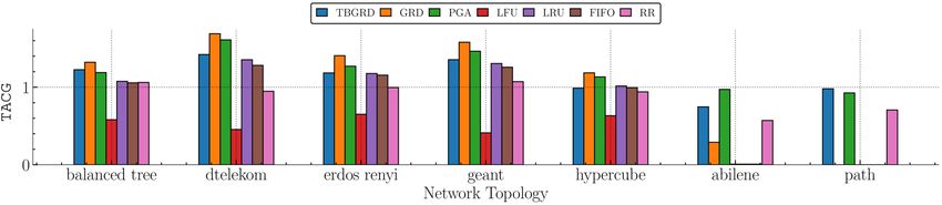

Online Caching Networks with Adversarial Guarantees 35:5

Fig. 1. A general cache network, as proposed by Ioannidis and Yeh [41]. Designated servers store items in
a catalog permanently. Requests arrive at arbitrary nodes in the network and follow predetermined paths
towards these servers; responses incur costs indicated by weights on the edges. Intermediate nodes can serve
as caches; the objective is to determine what items to store in each cache, to minimize the overall routing
cost or, equivalently, maximize the caching gain.

 Í
|S| = ∈ . We assume the slots in S are ordered lexicographically, i.e.,
 ( , ) ≺ ( ′, ′) if and only if < ′ or = ′ and < ′ . (1)
We can describe content allocation as a set ⊂ S × C, where = ( , ) ∈ indicates that item
 ∈ C is stored in slot ∈ S. The set of feasible allocations is
 D = { ⊆ S × C : | ∩ ({ } × C)| ≤ 1, ∀ ∈ S} . (2)
This ensures that each slot is occupied by at most one item; note that the cache capacity constraint
at each node ∈ is captured by the definition of S .

3.3 Requests and Responses
A request = ( , ) is determined by (a) the item ∈ C requested, (b) the path along which the
 | |
request is forwarded. A path is a sequence { } =1 of adjacent nodes ∈ . As in Ioannidis and
Yeh [41], we assume that paths are simple, i.e., they do not contain repeated nodes, and well-routed,
i.e., they terminate at a node in D . A request ( , ) is generated at node 1 and follows the path
 ; when the request reaches a node storing item , a response is generated. This response carries
item to query node 1 following the reverse path. We assume that time is slotted, and requests
arrive over a total of ∈ N rounds. We denote by R the set of all possible requests in the system.
At each round ∈ [ ], a set of requests R ⊆ R arrive in the system. Requests in R can arrive in
any order, and at any point in time within a round.1 However, we assume that the total number of
requests at each round is bounded by , ¯ i.e., |R | ≤ . ¯ Note that, when ¯ = 1, at most one request
arrives per round.

3.4 Routing Costs
We assume request routing does not incur any cost, but response routing does. In particular let
 ∈ R+ denote the cost of routing the response along the edge ( , ) ∈ .
1 Ouranalysis readily extends to a multiset R , whereby the same request is submitted multiple times within the same
round. We restrict the exposition to sets for notational simplicity.

 Proc. ACM Meas. Anal. Comput. Syst., Vol. 5, No. 3, Article 35. Publication date: December 2021.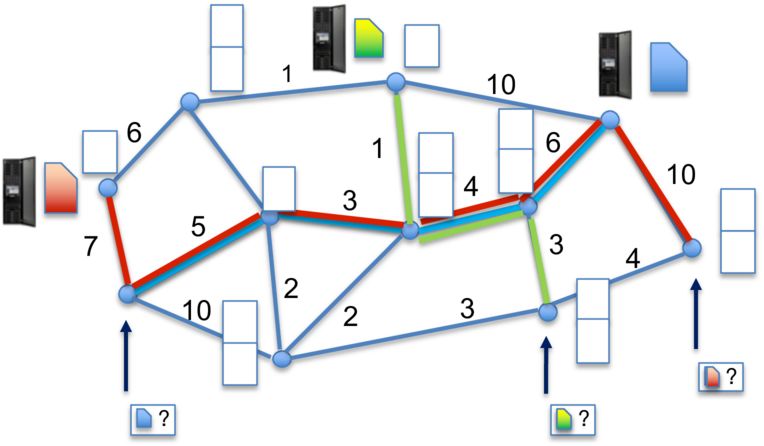

35:6 Yuanyuan Li et al.

 Table 1. Notation Summary

 Notational Conventions
 [ ] Set {1, . . . , }
 + Union ∪ { }
 Cache Networks
 ( , ) Network graph, with nodes and edges 
 C The item catalog
 Cache capacity at node ∈ 
 = ( , ) -th storage slot on node 
 S The set of storage slots
 S The set of storage slots in node 
 S The set of storage slots in path 
 S , The set of storage slots in path storing item 
 The set of item allocations
 D The set of feasible allocations
 R The set of requests arriving at round 
 ¯ The upper bound of |R |
 |R | Average number of requests per round
 The routing cost along edge ( , )
 ¯ The upper bound of possible routing cost
 Caching gain at round 
 Online Optimization
 The rounds horizon
 -regret
 E Hedge selector
 The weight vector maintained by hedge selector
 ℓ The reward vector fed to hedge selector
 The active color of slot 
 Number of colors
 I Information collected by control message
 
 The cumulative cost of edges upstream of on path 
 UC Update costs
 ˜ The extended -regret considering update costs

 Then, given an allocation ∈ S × C, the cost of serving a request ( , ) ∈ R is:
 | 
 Õ |−1 
  
 
  Ø
  
 
 ( , ) ( ) = +1 1­ ∩ S ′ × { } = ∅® .
 © ª
 (3)
 
  ′ ∈ [ ] 
 =1 « 
 
  ¬
Intuitively, Eq. (3) states that ( , ) ( ) includes +1 , the cost of edge ( +1, ), only if no cache
preceding +1 in path stores item . We denote by
 | 
 Õ |−1
 ¯ = max +1 (4)
 ( , ) ∈R
 =1
the maximum possible routing cost; note that this upper-bounds ( , ) ( ), for all ( , ) ∈ R,
 ∈ S × C.

Proc. ACM Meas. Anal. Comput. Syst., Vol. 5, No. 3, Article 35. Publication date: December 2021.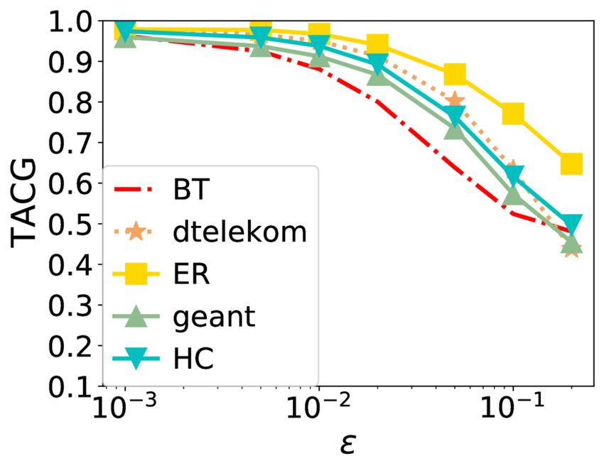

Online Caching Networks with Adversarial Guarantees 35:7

 The caching gain [41] of a request ( , ) due to caching at intermediate nodes is:
 | 
 Õ |−1  Ø
  
 
 
  
 
 ( , ) ( ) = ( , ) (∅) − ( , ) ( ) = +1 1­ ∩ S ′ × { } ≠ ∅® .
 © ª
 (5)
 
  ′ ∈ [ ] 
 =1 « 
 
  ¬
where ( , ) (∅) is the routing cost in the network when all caches are empty. The caching gain
captures the cost reduction in the network due to caching allocation .

3.5 Offline Problem
In the offline version of the cache gain maximization problem [41, 73], the request sequence {R } =1
is assumed to be known in advance; the goal is then to determine a feasible allocation ∈ D that
maximizes the total caching gain. Formally, given an allocation ∈ S × C, let
 Õ
 ( ) = ( ), (6)
 ∈R 
be the caching gain at round . Then, the offline caching gain maximization problem amounts to:
 
 Õ Õ
 Õ
 maximize ( ) = ( ) = ( ), (7a)
 
 =1 =1 ∈R 
 subject to ∈ D. (7b)
The following lemma implies this problem is approximable in polynomial time:
 Lemma 3.1 ([41, 73]). Function : S × C → R+ is non-decreasing and submodular. Moreover, the
feasible region D is a partition matroid.
 Hence, Problem (7) is a submodular maximization problem under matroid constraints. It is known
to be NP-hard [41, 73], and several approximation algorithms with polynomial time complexity
exist. The classic greedy algorithm [14] produces a solution within 12 -approximation from the
optimal. The so-called continuous greedy algorithm [15] further improves this ratio to 1 − 1 . A
different algorithm based on a convex relaxation of Problem (7) is presented in [41, 73]. The Tabular
Greedy algorithm [77] also constructs a 1 − 1 approximate solution in poly-time. We describe it in
details in Appendix A, as both TGOnline [77] and our DistributedTGOnline build on it.

3.6 Online Problem
In the online setting, requests are not known in advance, and we seek algorithms that make caching
decisions in an online fashion. In particular, at the beginning of round , an online algorithm selects
the current allocation ∈ D. Requests R ⊂ R subsequently arrive, and the cache gain ( ) is
rewarded, where : S × C → R+ is given by Eq. (6).
 As in standard online learning literature [39, 66], while choosing , the network has no knowl-
edge of the upcoming requests R , but can rely on past history. Formally, we seek an online
algorithm A that maps the history of past requests H = {R 1, .., R −1 } to a new allocation, i.e.,
 = A (H ). In particular, we aim for an algorithm A with sublinear -regret, given by
 " 
 # 
 " #
 Õ Õ Õ Õ
 ∗ ∗ 
 = E ( ) − ( ) = ( ) − E ( ) , (8)
 =1 =1 =1 =1
where is an approximation factor, and ∗
 is the optimal solution to (the offline) Problem (7). Note
that the expectation is over the (possibly) randomized choices of the algorithm A; we make no
probabilistic assumptions on request arrivals {R } =1 , and wish to minimize regret in the adversarial
setting, i.e., w.r.t. to the worst-case sequence {R } =1 . Put differently, our regret bounds will be

 Proc. ACM Meas. Anal. Comput. Syst., Vol. 5, No. 3, Article 35. Publication date: December 2021.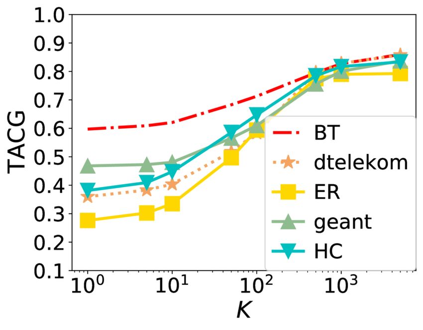

35:8 Yuanyuan Li et al.

 Algorithm 1: Hedge Selector E
 Input: Parameter ∈ R+ , action set C, horizon ∈ N.
1 def E.initialize():
2 Set ← 1 for all ∈ C
3 def E.arm():
4 return ∈ C with probability = Í 
 ∈C 

5 def E.feedback(ℓℓ ):
6 Set ← ℓ for all ∈ C

against an arbitrarily powerful adversary, that can pick any sequence {R } =1 , as long as the total
number of requests at each round is bounded by , ¯ i.e., |R | ≤ ¯ for all = 1, . . . , .
 Several remarks are in order regarding Eq. (8). First, the definition of the regret in Eq. (8), which
compares to a static offline solution, is classic. Several bandit settings, e.g., simple multi-armed
bandits [6, 50, 69], contextual bandits [1, 23, 26], submodular bandits [21, 76, 80] and, of course,
their applications to caching problems [10, 62, 66, 71], adopt this definition. In all these cases, the
dynamic, adaptive algorithm is compared to a static policy that has full hindsight of the entire trace
of actions. Nevertheless, as is customary in the context of online problems in which the offline
problem is NP-hard [21], the regret is not w.r.t. the optimal caching gain, but the gain obtained
by an offline approximation algorithm. Second, from the point of view of bandits, we operate in
the full-information feedback setting [39]: upon the arrival of requests R , the entire function
 : S × C → R+ is revealed,2 as the latter is fully determined by request set R . Third, Eq. (8)
captures the cost of serving requests, but not the cost of adaptation: changing an allocation from
 to +1 changes cache content, which in turn may require the movement of items. Neglecting
adaptation costs may be realistic if, e.g., adaptation happens in off-peak hours (e.g., the end of
a round occurs at the end of a day), and does not come with the same latency requirements as
serving requests in R . Nevertheless, we revisit this issue, incorporating update costs in the regret,
in Section 5. Finally, we stress that we seek online algorithms A that have sublinear regret but are
also distributed: each cache should be able to determine its own contents using past history it has
observed, as well as some limited information it exchanges with other nodes.

4 DISTRIBUTED ONLINE ALGORITHM
We describe our distributed online algorithm, DistributedTGOnline, in this section. We first give
an overview of the algorithm and its adversarial guarantees; we then fill out missing implementation
details.

4.1 Hedge Selector
Our construction uses as a building block the classic Hedge algorithm3 for the expert advice problem
[5, 39, 77]. This online algorithm selects an action from a finite set at the beginning of a round. At
the conclusion of a round, the rewards of all actions are revealed; the algorithm accrues a reward
based on the action initially selected, and adjusts its decision.
 In our case the set of possible actions coincides with the catalog C, i.e., the algorithm selects an
item ∈ C per round ∈ N. The hedge selector maintains a weight vector = [ ] ∈ C ∈ R | C | ,
where weight corresponds to action ∈ C. The hedge selector supports two operations (see
2 In contrast to the classic bandit feedback model, where only the reward ( ) is revealed in each round .
3 This is also known as the multiplicative weight algorithm.

Proc. ACM Meas. Anal. Comput. Syst., Vol. 5, No. 3, Article 35. Publication date: December 2021.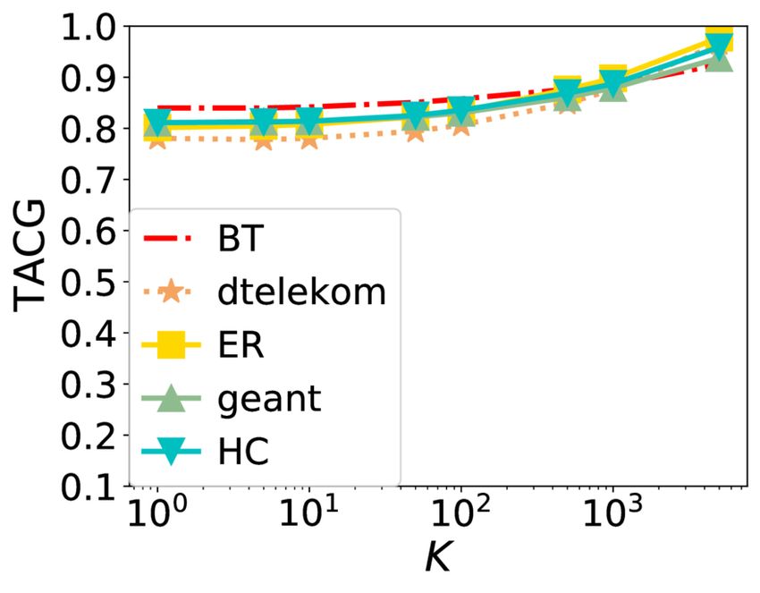

Online Caching Networks with Adversarial Guarantees 35:9

 Algorithm 2: DistributedTGOnline
 foreach ∈ S do
 foreach ∈ [ ] do
 E , .initialize().
 set = 1, choose uniformly at random from [ ]
 ← E , .arm() ; // Sets ← {( , )} ∈S
 for = 1, 2, ..., do
 /* During round : */
1 foreach = ( , ) ∈ R do
 2 Send request upstream over until a hit occurs.
 3 Send response carrying downstream, and incur routing costs.
 4 Send control message upstream over to construct I and W, given by (12).
 5 Send control message carrying I and W downstream over , and do the
 following:foreach ∈ S do
 6 Use I and W to construct ℓ ( , ) ∈ R+| C | via (15).
 7 Call E , .feedback(ℓℓ ( , ))
 /* At the end of round : */
 Ð
8 foreach ∈ ( , ) ∈R S do
 9 if mod = 0 then
10 Select u.a.r. from [ ] ; // Shuffle color 
11 ← E , .arm() ; // Update allocation at 
12 ← + 1

Alg. 1. The first, E.arm( ), selects an action from action set C. The second, E.feedback(ℓℓ ), ingests
the reward vector ℓ = [ℓ ] ∈ C ∈ R+| C | , where ℓ is the reward for choosing action ∈ C at round ,
and adjusts action weights as described below. In each iteration , the hedge selector alternates
between (a) calling = E.arm( ), to produce action , (b) receiving a reward vector ℓ , and using it
via E.feedback(ℓℓ ) to adjust its internal weight vector. In particular, E.arm( ) selects action ∈ C
with probability:
 
 = Í , (9)
 ∈ C 
i.e., proportionally to weight . Moreover, when E.feedback(ℓℓ ) is called, weights are updated via:
 +1 = ℓ ,
 
 for all ∈ C, (10)
where > 0 is a constant. In a centralized setting
 √ where an adversary selects the vector of weights
ℓ , the no-regret hedge selector attains an ( ) regret for an appropriate choice of > 0 (see
Lemma B.1 in Appendix B). We use this as a building block in our construction below.

4.2 DistributedTGOnline Overview
To present the DistributedTGOnline algorithm, we first need to introduce the notion of “colors”.
The algorithm associates each storage slot = ( , ) ∈ S with a “color” from set [ ] of 
distinct values (the “color palette”). The online algorithm makes selections in the extended action
space S × C × [ ], choosing not only an item to place in a slot, but also how to color it.

 Proc. ACM Meas. Anal. Comput. Syst., Vol. 5, No. 3, Article 35. Publication date: December 2021.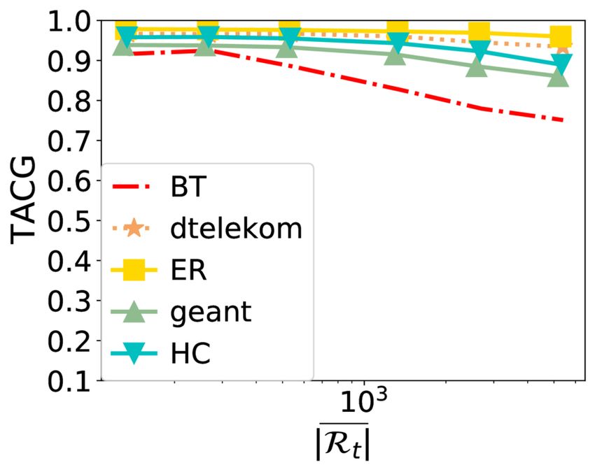

35:10 Yuanyuan Li et al.

 This coloring is instrumental to attaining a 1 − 1 -regret. In offline tabular greedy algorithm of
Streeter et al. [77], which we present in Appendix A, when = 1, i.e., there is only one color,
the algorithm reduces to simply the locally greedy algorithm (see Section 3.1 in [77]), achieving
only a 12 approximation ratio. When → ∞, the algorithm can intuitively be viewed as solving a
continuous extension of the problem followed by a rounding (via the selection of the color instance),
in the same spirit as the so-called ContinuousGreedy algorithm [15]. A finite size “color palette”
represents a midpoint between these two extremes. We give more insight into this relationship
between these two algorithms in Section 4.5.
 In more detail, every storage slot ∈ S maintains (a) the item ∈ C stored in it, (b) an active
color ∈ [ ] associated with this slot, and (c) different no-regret hedge selectors {E , } =1 ,

one for each color. All selectors {E , } =1 operate over action set C: that is, each such selector can
 
have its arm “pulled” to select an item to place in a slot. Though every slot maintains different
selectors, one for each color, it only uses one at a time. The active colors { } ∈S are initially
selected u.a.r. from [ ], and remain active continuously for a total pull/feedback interactions,
where ∈ N; at that point, is refreshed, selected again u.a.r., bringing another selector into play.
All in all, the algorithm proceeds as follows during round .
 (1) When a request ( , ) ∈ R is generated, it is propagated over the path until a hit occurs; a
 response is then backpropagated over the path , carrying , and incurring a routing cost.
 (2) At the same time, an additional control message is generated and propagated upstream over
 the entire path . Moving upstream, it collects information from slots it traverses.
 (3) After reaching designated server at the end of the path, the control message is backpropagated
 over the path in the reverse direction. Every time it traverses a node ∈ , storage slot
 ∈ S fetches information stored in the control message and computes a reward vector
 ℓ ( , ). This is then fed to the active hedge selector via E , .feedback( ℓ ( , )).
 (4) At the end of the round, we check if the arm of E , has been pulled for a total of times
 under active color ; if so, a new color is selected u.a.r. from [ ].
 (5) Irrespective of whether changes or not, at the end of the round, each slot updates its
 contents via the current active hedge selector E , , by calling operation E , .arm() to choose
 a new item to place in .
We define the control messages exchanged, the information they carry, and the reward vectors fed
to hedge selectors in Section 4.3. Only slots in a request’s path need to exchange messages, provide
feedback to their selectors, and (possibly) update their contents at the end of a round. Moreover,
messages exchanged are of size (| |). We allow ≥ ; in this case, colors are selected u.a.r. only
once, at the beginning of the execution of the algorithm, and remain constant across all rounds.4
Finally, note that updating cache contents at the end of a round does not affect the incurred cost;
we remove this assumption in Section 5. √
 Our first main result is that DistributedTGOnline has a (1 − 1/ )-regret that grows as ( ):
 Theorem 4.1. Consider the sequence of allocations { } =1 produced by the DistributedTGOnline
 q
 log | C |
algorithm using hedge selectors determined by Alg. 1, with = 1¯ . Then, for all ≥ log |C|
and all ≥ 1:
 " # ( )
 Õ Õ p
 
 E ( ) ≥ (|S|, ) · max ( ) − 2 ¯ |S| 
 ¯ log |C|, (11)
 ∈ D
 =1 =1
 | S |

where (|S|, ) = 1 − (1 − 1 
 ) − 2 −1 .
4 In such a case, selectors corresponding to inactive colors need not be maintained, and can be discarded.

Proc. ACM Meas. Anal. Comput. Syst., Vol. 5, No. 3, Article 35. Publication date: December 2021.

Online Caching Networks with Adversarial Guarantees 35:11

 The main intuition behind the proof is to view DistributedTGOnline as a version of the offline
TabularGreedy that, instead of greedily selecting a single item , ∈ C per step, it greedily selects
an entire item vector ® , ∈ C across all rounds, where is the number of rounds. To cast the proof
in this context, we define new objective functions and whose domain is over decisions across 
rounds, as opposed to the original per time-slot functions (whose domain is only over one round).
Due to the properties of the no-regret hedge selector, and the formal guarantees of the offline case
(c.f. Thm. A.1), these new objectives attain 1 − 1 bound shown in Eq. (26), yielding the bound on the
regret. The detailed proof of this theorem is provided in Appendix C. Note that for large enough
(at least Ω(|S| 2 )), quantity (|S|, ) can be made arbitrarily close to 1 − 1/ . Hence, Theorem 4.1
has the following immediate corollary:

 Corollary 4.2. For any > 0, there exists an = Θ( |S | ) such that the expected (1− 1 − )-regret
 2

of DistributedTGOnline is ≤ 2 | S | log | |.
 ¯¯ 3p

 DistributedTGOnline is a distributed implementation of the (centralized) online tabular greedy
algorithm of Streeter et al. [77], which is itself an online implementation of the so-called tabular
greedy algorithm [77], which we present in Appendix A. We depart however from [77] in several
ways. First, the analysis by Streeter et al. requires that feedback is provided at every slot ∈ S .
We amend this assumption, as only nodes along a path need to update their selectors/allocations
in our setting. Second, we show that feedback provided to arms can be computed in a distributed
fashion, using only messages along the path , as described below in Section 4.3. These two facts
together ensure that DistributedTGOnline is indeed distributed. Finally, the analysis of Streeter
et al. assumes that colors are shuffled at every round, i.e., applies only to = 1. We extend this to
arbitrary ≥ 1. As we discuss in Section 5, this is instrumental to bounding regret when accounting
for update costs; the later becomes Θ( ) when = 1.

4.3 Control Messages, Information Exchanged, and Rewards
The algorithm is summarized in Alg. 2. We describe here the control messages, information ex-
changed, and reward vectors fed to hedge selectors during the generation of a request = ( , ) ∈ R .
 Ð
Let S = ∈ S be the set of all slots in nodes in . Let also S , = { ∈ S : ( , ) ∈ } ⊆ S be
the slots in path that store the requested item ∈ C. The control message propagated upstream
towards the designated server collects both the (a) color of every slot in S , and (b) the upstream
cost at each node ∈ . Formally, the information collected by the upstream control message is
 
 I = {( , )} ∈S , , and W = { } ∈ , (12)
 
where is the cumulative cost of edges upstream of on path , i.e.,
 Í | |−1
 = = ( ) +1 , (13)

where ( ) = {1, 2, ..., | |} is position of in , i.e., ( ) = if = . Note that both |I| and
|W| are (| |).
 Upon reaching the end of the path, a message carrying this collected information (I,W) is sent
downstream to every node in the path. For each slot ∈ S , let:
 S ⪯ = { ′ ∈ S , : ′ < or ′ = , ′ ≺ } (14)
be the slots in the path that store and either (a) are colored with a color smaller than , or (b)
are colored with , and precede in the ordering given by Eq. (1). Note that S ⪯ can be computed
having access to I. Then, the reward vector ℓ ( , ) ∈ R+| C | fed to hedge selector E , at slot

 Proc. ACM Meas. Anal. Comput. Syst., Vol. 5, No. 3, Article 35. Publication date: December 2021.

35:12 Yuanyuan Li et al.

 ∈ S comprises the following coordinates:
 (
 max ( ′, ′ ) ∈S⪯ + ′ , if ′ = 
 
 ℓ ′ ( , ) = for all ′ ∈ C, (15)
 max ( ′, ′ ) ∈S⪯ ′ , . .
which captures the marginal gain of adding an element to the allocation at time , assuming that
the latter is constructed adding one slot, item, and color selection at a time (following an ordering
w.r.t. colors first and slots second). This is stated formally in Lemma C.1 in Appendix C. Note again
that all these quantities can be computed at every ∈ S having access to I and W.5

4.4 A Negative Result
We conclude this section with a negative result, further highlighting the importance of Theorem 4.1.
DistributedTGOnline comes with adversarial guarantees; our experiments in Section 7 indicate
that also works well in practice. Nevertheless, for several topologies we explore, we observe that
a heuristic proposed by Ioannidis and Yeh [41], termed GreedyPathReplication, performs as
well or slightly better than DistributedTGOnline in terms of time-average caching gain. As we
observed this in both stationary as well as non-stationary/transient request arrivals, this motivated
us to investigate further whether this algorithm also comes with any adversarial guarantees.
 Our conclusion is that, despite the good empirical performance in certain settings, Greedy-
PathReplication does not enjoy such guarantees. In fact, the following negative result holds:
 Lemma 4.3. Consider the online policy GreedyPathReplication due to Ioannidis and Yeh [41],
which is parametererized by > 0. Then, for all ∈ (0, 1] and all > 0, GreedyPathReplication
has Ω( ) -regret.
 We prove this lemma in Appendix E. The adversarial counterexample we construct in the
proof informed our design of experiments for which GreedyPathReplication (denoted by GRD in
Section 7) performs poorly, attaining a zero caching gain throughout the entire algorithm’s execution
(see Fig. 3-5). The same examples proved hard for several other greedy/myopic policies, even though
DistributedTGOnline performed close to the offline solution in these settings. Both Lemma 4.3,
as well as the experimental results we present in Section 7, indicate the importance of Theorem 4.1
and, in particular, obtaining a universal bound on the regret against any adversarially selected
sequence of requests.

4.5 Color Palette
To provide further intuition behind the “color palette” induced by and the role it plays in our
algorithm, we describe here in more detail how it relates to the ContinuousGreedy algorithm,
the standard algorithm for maximizing submodular functions subject to a matroid constraint [15].
 Intuitively, given a submodular function : Ω → R+ and a matroid constraint set D, the
ContinuousGreedy algorithm maximizes the multilinear relaxation of objective, given by
 Õ Ö Ö
 ˜( ) = E [ ( )] = ( ) (1 − ). (16)
 ⊆Ω ∈ ∉ 

That is, the multilinear extension ˜ : [0, 1] |Ω | → R+ is the expected value of the objective assuming
that each element in A is sampled independently, with probability given by ∈ [0, 1], ∈ Ω.
ContinuousGreedy first obtains a fractional solution in the matroid polytope of D. This is
constructed by incrementally growing the probability distribution parameters , starting from
5 Inpractice, trading communication for space, the full W can also be just computed once, at the first time request ( , )
 
is generated, Each can store their own for paths that traverse them, and only weights of nodes storing need to be
included in W in subsequent requests.

Proc. ACM Meas. Anal. Comput. Syst., Vol. 5, No. 3, Article 35. Publication date: December 2021.

Online Caching Networks with Adversarial Guarantees 35:13

 = 0 , with a variant of the so-called Frank-Wolfe algorithm. Then, ContinuousGreedy rounds
the resulting fractional solution via, e.g., pipage rounding [2] or swap rounding [19], mapping it
to set solutions. We refer the reader to Calinescu et al. [15] for a more detailed description of the
algorithm.
 In comparison, the color palette also creates a distribution across item selections, as implied
by the colors. When the number of colors approaches infinity, the selection process of
DistributedTGOnline also “grows” this probability distribution (starting, again, from an empty
support) infinitesimally, by an increment inversely proportional to (see also the offline version
TabularGreedy in Appendix A). As goes to infinity, this recovers the 1 − 1/ approximation
guarantee of continuous greedy [64, 77]. For any finite , the guarantee provided by Theorem 4.1
lies in between this guarantee and 12 approximation of the locally greedy algorithm ( = 1).

5 UPDATE COSTS
We now turn our attention to incorporating update costs in our analysis. We denote by , ′ the cost

of fetching item at storage slot at the end of a round. Then, the total update cost of changing an
allocation to +1 at the end of round is given by:
 Õ
 UC( , +1 ) = ′
 , . (17)
 ( , ) ∈ +1 \ 
When such update costs exist, we need to account for them when adapting cache allocations. We
thus incorporate them in the -regret as follows:
 
 " −1
 # " −1 #
 Õ Õ Õ Õ
 ∗ +1 +1
 ˜ = ( ) − E ( ) − UC( , ) = + E UC( , ) . (18)
 =1 =1 =1 =1
 Note that, in this formulation, the optimal offline policy ∗
 has no update cost, as it is static.
We refer to ˜ as the extended -regret of an algorithm. This extension corresponds to adding the
expected update cost incurred by a policy A to its -regret.
 Unfortunately, the update costs of DistributedTGOnline (and, hence, its extended regret) grow
as Θ( ) in expectation. In particular, the following lemma, proved in Appendix D, holds:
 Lemma 5.1. When DistributedTGOnline is parametrized with the hedge selector in Alg. 1, it
incurs an expected update cost of Ω( ) for any choice of ∈ R+ .
 √
 Nevertheless, the extended regret can be reduced to ( ) by appropriately modifying Alg. 1,
the no-regret-hedge selector used in slots E , . In particular, the linear growth in the regret is due
to the independent sampling of cache contents within each round. Coupling this selection with
the presently selected content can significantly reduce the update costs. More specifically, instead
of selecting items independently across rounds, the new item can be selected from a probability
distribution that depends on the current allocation in the cache. This conditional distribution
can be design in a way that the (marginal) probability of the new item is the same as in Alg. 1,
thereby yielding the same expected caching gain. On the other hand, coupling can bias the selection
towards items already existing in the cache. This reduces update costs, especially when marginal
distributions change slowly.
 The coupled hedge selector described in Alg. 3 accomplishes exactly this. As seen in line 9 of Alg. 3,
pulling the arm of the hedge selector is dependent on (a) the previously taken action/selected item
and (b) the change in the distribution implied by weights , ∈ C. We give more intuition as to how
this is accomplished in Appendix D. In short, the coupled hedge selector solves a minimum-cost
flow problem via an iterative algorithm. The minimum-cost flow problem models a so-called optimal
transport or earth mover distance problem [67] from to +1 , the distributions over catalog C

 Proc. ACM Meas. Anal. Comput. Syst., Vol. 5, No. 3, Article 35. Publication date: December 2021.

35:14 Yuanyuan Li et al.

 Algorithm 3: Coupled Hedge Selector
 Input: Parameter ∈ R+ , action set C, horizon ∈ N.
 1 def E.initialize():
 2 Set ← 1 and old ← | C1 | for all ∈ C
 3 Pick old u.a.r. from C
 4 def E.feedback(ℓℓ ):
 5 Set ← ℓ for all ∈ C
 6 def E.correlated_arm():
 7 Set new ← Í for all ∈ 
 ∈C
 8 Pick new ← coupled_movement ( old , new , old ) ; // Marginal is new
 9 old ← new
10 old ← new
11 return new
12 def coupled_movement( old , new , old ):
13 Compute = { ∈ C : new − old > 0}.
14 Set ← | new − old |, for all ∈ C
 Í
15 Compute
 Í a feasible flow [ , ] ( , ) ∈ C 2 , where
 Í ∈ , = for ∈ C \ , and
 ∈ C\ , = for ∈ , to transport ∈ C\ mass from the components in to the
 components in C \ .
16 ← old .
17 temp ← old
18 for ∈ C \ do
19 for ∈ do
20 , temp ← elementary_ movement( , temp, , , , )
21 return temp
22 def elementary_ movement( , temp, , , ):
23 if temp = then
 − 
 (
 , + ( − ) w.p. 
24 temp, ←
 , + ( − ) w.p. 
25 else
26 temp, ← temp, + ( − )
27 return , temp

at rounds and + 1, respectively, The resulting solution comprises conditional distributions for
“jumps” among elements in C, which are used to determine the next item selection using the current
choice: by being solutions of the minimum-cost flow problem, they incur small update cost, while
ensuring that the posterior distribution after the “jump” is indeed +1 .
 Our second main result establishes that using this hedge selector
 √ instead of Alg. 1 in Distribut-
edTGOnline ensures that the extended regret grows as ( ).
 Theorem 5.2. Consider q DistributedTGOnline with hedge selectors E , implemented via Alg. 3
 log | C | √
parameterized with = ¯
 1
 . Assume also that colors are updated every = Ω( ) rounds.

Proc. ACM Meas. Anal. Comput. Syst., Vol. 5, No. 3, Article 35. Publication date: December 2021.

Online Caching Networks with Adversarial Guarantees 35:15

Table 2. Graph Topologies and Experiment Parameters. We indicate the number of nodes in each graph (| |),
the number of edges (| |), the number of query nodes (|Q|), and the ranges of cache capacities and edge
weights . In the last four columns we also report , , , and : which are the caching
gain attained by OFL with Stationary Request, Sliding Popularity, Shot Noise, and CDN trace, respectively.

 topologies | | | | |Q| 
 ER 100 1042 5 1-5 1-100 1569.93 1123.76 72.03 976.65
 BT 341 680 5 1-5 1-100 5547.89 3211.63 220.58 3504.58
 HC 128 896 5 1-5 1-100 2453.66 2045.69 152.38 1895.41
 dtelekom 68 546 5 1-5 1-100 969.55 772.53 49.55 1005.24
 GEANT 22 66 5 1-5 1-100 1564.02 981.60 66.50 1185.56
 abilene 9 26 2 0-5 100 81.21 81.21 41.39 -
 path 4 6 1 0-5 100 20.00 20.00 10.00 -

Then, the standard regret is again bounded as in Corollary 4.2. Moreover, the update cost of
DistributedTGOnline is such that
 " −1 #
 Õ
 +1
 √
 E UC( , ) = ( ), (19)
 =1
 √
and, as a consequence, the extended regret is ˜ = ( ).
 √
 The proof can be found in Appendix F. We note that the theorem requires that = Ω( ),
i.e., that colors are shuffled infrequently. Whenever a color changes, DistributedTGOnline, the
corresponding change in the active hedge selector can lead to sampling vastly different allocations
than the current ones. Consequently, such changes√ can give rise to large update costs whenever a
color is changed. The requirement that = Ω( ) allows for some frequency in changes, but not,
e.g., at a constant number of rounds (as, e.g., in Streeter et al. [76], where = 1). Put differently,
Theorem 5.2 allows
 √ for experiencing momentarily large update costs, as long as we do not surpass
a budget of ( ) color updates overall. We note that the couple hedge selector in Alg. 3 has the
same time complexity as the hedge selector given in Alg. 1, which is (|C|) per iteration.

6 EXTENSIONS
Jointly Optimizing Caching and Routing. Our model can be extended to consider joint op-
timization of both cache and routing decisions, following an extended model by Ioannidis and
Yeh [43]. Under appropriate variable transformations, the new objective is still submodular over the
extended decision space. Moreover, the constraints over the routing decisions can similarly be cast
as assignments to slots. Together, these allow us to directly apply DistributedTGOnline and attain
the same 1 − 1/ approximation guarantee. We describe this extension in detail in Appendix H.
Anytime Regret Guarantee. Our algorithm assumes prior knowledge of the time horizon ; this
is necessary to set parameter in Theorem 4.1. Nevertheless, we can use the well-known doubling
trick [16] to obtain anytime regret guarantees. In short, the algorithm starts from a short horizon;
at the conclusion of the horizon, the algorithm restarts, this time doubling the horizon. We show
 √ in
Appendix I that, by using this doubling trick, DistributedTGOnline indeed attains an ( )
regret, without requiring prior knowledge of . This remains true when update costs are also
considered in the regret.

 Proc. ACM Meas. Anal. Comput. Syst., Vol. 5, No. 3, Article 35. Publication date: December 2021.

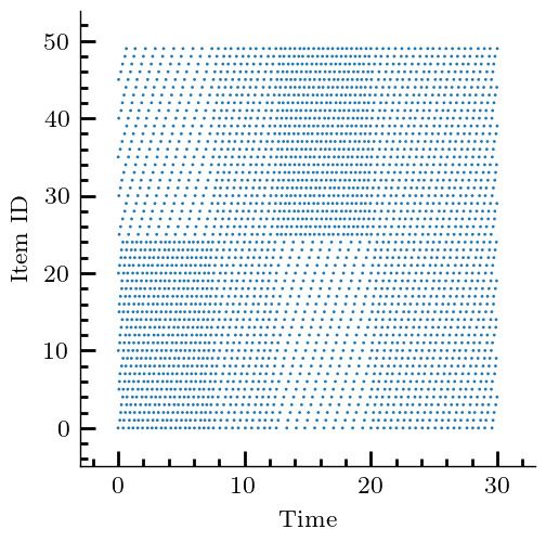
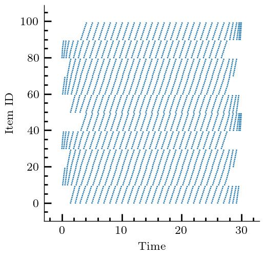
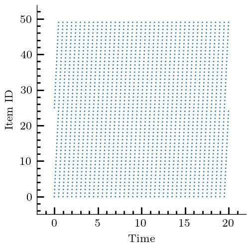
35:16 Yuanyuan Li et al.

 (a) Stationary Requests (b) Sliding Popularity

 (c) Shot Noise (d) CDN trace

Fig. 2. Request traces for different scenarios. Each dot indicates an access to an item in the catalog; items are
ordered in an overall increasing popularity from top to bottom. In Sliding Popularity, popularity changes at
fixed time intervals, through a cyclic shift (most popular items become least popular). In Shot Noise, each
item remains active for a limited lifetime.

7 EXPERIMENTS
7.1 Experimental Setting
Networks. We use four synthetic graphs, namely, Erdős-Rényi (ER), balanced tree (BT), hypercube
(HC), and a path (path), and three backbone network topologies: [70] Deutsche Telekom (dtelekom),
GEANT, Abilene. The parameters of different topologies are shown in Tab. 2. For the first five
topologies (ER–GEANT), weights for each edge is uniformly distributed between 1–100. Each item
 ∈ C is permanently stored in a designated servers D which is designated uniformly at random
(u.a.r.) from . All nodes in are also has storage space, which is u.a.r. sampled between 1 to
5. Requests are generated from nodes Q u.a.r. selected from . Given the source 1 ∈ Q and the
destination | | ∈ D of the request , path is the shortest path between them. For the remaining
two topologies (abiline and path), we select parameters in a way that is described in Appendix G.
Demand. We consider three different types of synthetic request generation processes, and one
trace-driven. In the Stationary Requests scenario (see Fig. 2(a), each = ( , ) ∈ R is associated with
an exogenous Poisson process with rate 1.0, and is chosen from C via a power law distribution
with exponent 1.2. In the Sliding Popularity scenario, requests are again Poisson with a different
exponent 0.6, and popularities of items are periodically reshuffled (see Fig. 2(b)). In the Shot Noise
scenario, each item is assigned a lifetime, during which it is requested according to a Poisson
process; upon expiration, the item is retired (see Fig. 2(c)). In the CDN scenario (see Fig. 2(d)), we

Proc. ACM Meas. Anal. Comput. Syst., Vol. 5, No. 3, Article 35. Publication date: December 2021.

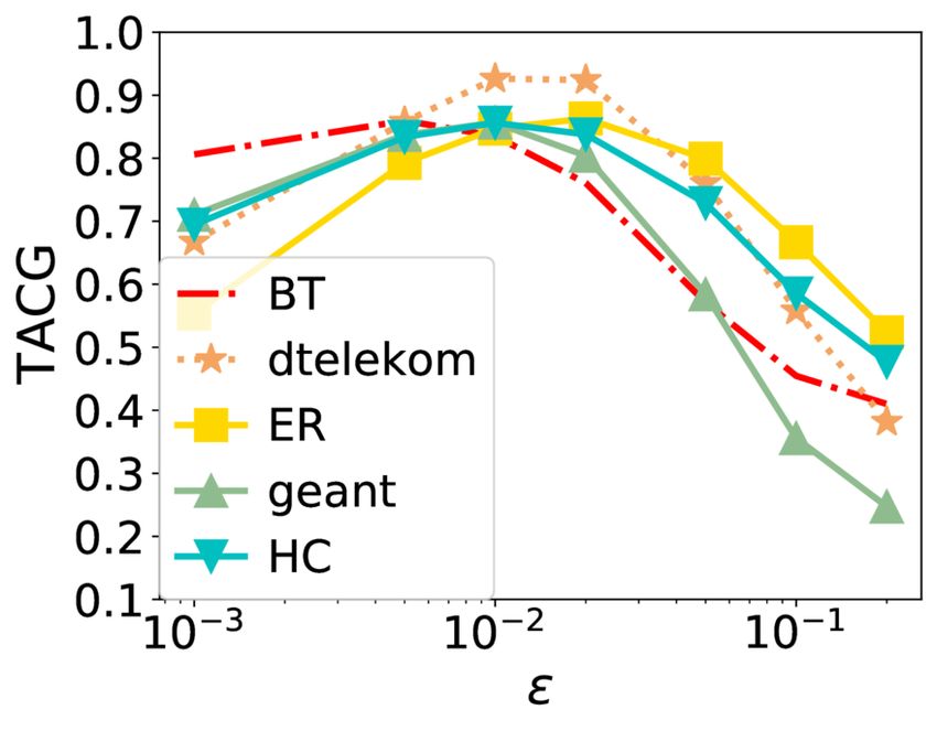
Online Caching Networks with Adversarial Guarantees 35:17

Fig. 3. TACG of different algorithms over different topologies with Stationary Requests. The total simulation
time is 1000 time units. TBGRD, GRD, and PGA perform well in comparison to path replication policies. However,
GRD and other myopic strategies attain zero TACG over abilene and path, the round-robin scenarios. In
comparison, TBGRD and PGA still perform well.

generate requests using a real-life trace from a CDN provider. The trace spans 1 week, and we
extract from it about 10 × 105 requests for the = 103 most popular files.
 For abiline and path, we replace the Poisson arrivals on the three synthetic traces (Stationary
Requests, Sliding Popularity, Shot Noise) with requests generated in a round-robin manner, as
described in Appendix G.2. This is designed in an adversarial fashion, that leads to poor performance
for greedy/myopic algorithms.
Algorithms. We implement the following online algorithms 6 :
 • Path replication with least recently used (LRU), least frequently used (LFU), first-in-first-
 out (FIFO), and random-replacement (RR) eviction policies: In all these algorithms, when
 responses are back-propagated over the reverse path, all nodes they encounter store requested
 item, evicting items according to one of the aforementioned policies.
 • Projected gradient ascent (PGA): This is the distributed, adaptive algorithm oringinally pro-
 posed by Ioannidis and Yeh [41]. This is attains an (1 − 1/ )-approximation guarantee in
 expectation when requests are stationary, but comes with no guarantee against adversarial
 requests. Similar to our setting, it also operated in rounds, at the end of which contents are
 shuffled.
 • Greedy path replication (GRD): This is a heuristic, also proposed by Ioannidis and Yeh [41].
 Though it performs well in many cases, we prove in Appendix D that its (1 − 1/ )-regret is
 Ω( ) in the worst case.
 • DistributedTGOnline (TBGRD): this is our proposed algorithm. We implement it with both
 independent hedge selector shown in Algorithm 1 and coupled hedge selector in Algorithm 3.
 Unless indicated otherwise, we set = 0.005, number of colors = 100, ¯ = 1, and = for
TBGRD. For PGA and GRD, we explore parameters and range from 0.005-5 and 0.005-1 individually,
and pick the optimal values. In experiments where we do not measure update costs, we implement
TBGRD with the independent hedge selector (Alg. 1), as it yields the same performance as the coupled
hedge selector (Alg. 3) in expectation (see also Fig. 9(a) and 9(b)).
 Finally, we also implement the offline algorithm (OFL) by Ioannidis and Yeh [41], and use the
resulting (1 − 1/ )-approximate solution as baseline (see metrics below).
Performance Metrics. We use normalized time-average cache gain (TACG) as the metric to
measure the performance of different algorithms. More specifically, leveraging PASTA [78], we
measure ( ) at epochs generated by a Poisson process with rate 1.0 for 5000 time slots, and
average these measurements. To compare performance across different topologies, we normalize

6 Our code is publicly available at https://github.com/neu-spiral/OnlineCache.

 Proc. ACM Meas. Anal. Comput. Syst., Vol. 5, No. 3, Article 35. Publication date: December 2021.

35:18 Yuanyuan Li et al.

Fig. 4. TACG of different algorithms over different topologies with Sliding Popularity. The total simulation
time is 1000 time units. TBGRD, GRD, and PGA again outperform path replication algorithms; GRD sometimes
even outperforms the (static) OFL solution, attaining a normalized TACG larger than one. However, GRD and
several path replication algorithms again fail catastrophically over the abilene and path scenarios, while
TBGRD and PGA again attain a normalized TACG close to one.

Fig. 5. TACG of different algorithms over different topologies with Shot Noise. We again observe TBGRD, GRD,
and PGA perform well in this non-stationary request arrival setting. Moreover, several algorithms outperform
the (static) offline solution OFL in this setting. Again, GRD and other myopic path replication policies fail over
abilene and path, while TBGRD and PGA still attain a non-zero TACG.

Fig. 6. TACG of different algorithms over different topologies with CDN trace. The total simulation time is
2000 time units. We again observe that TBGRD, GRD, and PGA outperform path replication policies.

the average by OFL , the caching gain attained by OFL, yielding:

 TACG = 1OFL =1 ( ).
 Í
 (20)

The corresponding OFL values are reported in Table 2. We also measure the cumulative update cost
(CUC) of TBGRD over time under the hedge and coupled hedge selectors, i.e.,
 Í −1
 CUC = =1 UC( , +1 ), (21)
where we measure the instantaneous update cost UC using (17) with weights set to 1.

Proc. ACM Meas. Anal. Comput. Syst., Vol. 5, No. 3, Article 35. Publication date: December 2021.

Online Caching Networks with Adversarial Guarantees 35:19

 (a) Average number of requests |R | (b) Number of colors 

 (c) Parameter (d) Color update period 

Fig. 7. TACG vs. different parameters under Stationary Request. As the average number of requests increases,
TACG decreases. Number of colors does not affect a lot. As increases, TACG decreases. As color update
period increases, TACG increases.

7.2 Results
TACG Comparison. Figures 3-5 show the performance of different algorithms w.r.t. TACG across
multiple topologies, for different synthetic traces (Stationary, Sliding Popularity, and Shot Noise,
respectively). For GRD here, we explore parameters range from 0.0001-1, and pick the optimal
values. We observe that TBGRD, GRD, and PGA have similar performance across topologies on all
three traces for the first five topologies, with GRD being slightly higher performing than the other
two; nevertheless, on the last two topologies, that have been designed to lead to poor performance
for myopic/greedy strategies, both GRD and other myopic strategies (e.g., LFU, LRU, and FIFO) are
stymied, attaining a zero caching gain throughout. This also verifies the suboptimality of GRD
stated in Lemma 4.3. In contrast, TBGRD and PGA still attain a TACG close to the offline value; not
surprisingly RR also has a suboptimal, but non-zero gain in these scenarios as well.
 The more a trace departs from stationarity, the more the performance of OFL degrades: As seen
in Tab. 2, the caching gain obtained by OFL consistently across the different topologies has the
highest value in the Stationary trace, then decreases as we change to CDN, Sliding Popularity SN
traces, in that order.
 We also note that in the Shot Noise case several algorithms attain a normalized TACG that is
higher than 1. This indicates that the dynamic algorithms beat the static offline policy in this setting.
The above observations largely carry over to the CDN trace, shown in Figure 6, for which however
we do not consider the two round-robin demand scenarios (abilene and path), as the demand is
driven by the trace.

 Proc. ACM Meas. Anal. Comput. Syst., Vol. 5, No. 3, Article 35. Publication date: December 2021.