Non-principal axis rotation in binary asteroid systems and how it weakens the BYORP effect
←
→
Page content transcription
If your browser does not render page correctly, please read the page content below
Non-principal axis rotation in binary asteroid systems and how it weakens the
                                                                                    BYORP effect

                                                                                   Alice C. Quillena,∗, Anthony LaBarcaa , YuanYuan Chenb
                                                                       a Department of Physics and Astronomy, University of Rochester, Rochester, NY 14627, USA
                                                     b Key   Laboratory of Planetary Sciences, Purple Mountain Observatory, Chinese Academy of Sciences, Nanjing 210008, China

                                               Abstract
                                               Using viscoelastic mass/spring model simulations, we explore tidal evolution and migration of compact binary asteroid
arXiv:2107.14789v1 [astro-ph.EP] 30 Jul 2021

                                               systems. We find that after the secondary is captured into a spin-synchronous state, non-principal axis rotation in the
                                               secondary can be long-lived. The secondary’s long axis can remain approximately aligned along the vector connecting
                                               secondary to primary while the secondary rocks back and forth about its long axis. Inward orbital semi-major axis
                                               migration can also resonantly excite non-principal axis rotation. By estimating solar radiation forces on triangular
                                               surface meshes, we show that the magnitude of the BYORP effect induced torque is sensitive to the secondary’s spin
                                               state. Non-principal axis rotation within the 1:1 spin-orbit resonance can reduce the BYORP torque or cause frequent
                                               reversals in its direction.

                                               1. Introduction                                                       Orbital eccentricity could cause an elongated secondary to
                                                                                                                     tumble, delaying BYORP drift-induced evolution and ex-
                                                   The field of research on binary asteroids currently has           tending the lifetime of NEA binaries (Naidu and Margot,
                                               two dynamical conundrums. Light curve based estimates                 2015).
                                               of viscoelastic behavior in single asteroids based on tum-                Possible ways to account for the spin synchronous rota-
                                               bling damping give elastic modulus times energy dissipa-              tion and the inferred tidal spin-down of the secondary are
                                               tion parameter, µQ ∼ 1011 Pa (Harris, 1994; Pravec et al.,            earlier formation in the Main Belt, formation at a slower
                                               2014), exceeding those estimated in binary asteroids (Gol-            spin rate, formation at a smaller orbital semi-major axis
                                               dreich and Sari, 2009; Taylor and Margot, 2011; Jacobson              where the spin down time is shorter, or if the secondary
                                               and Scheeres, 2011; Nimmo and Matsuyama, 2019) by 1                   has lower µQ ∼ 109 Pa (Taylor and Margot, 2011). Rub-
                                               to 4 orders of magnitude. Drift rates estimated due to ra-            ble pile NEAs may have low µQ values due to stress on
                                               diation forces, known as binary-YORP or BYORP, are so                 contact points arising from internal voids (Goldreich and
                                               rapid that binary NEA asteroid lifetimes should be short,             Sari, 2009), a dissipative regolith surface layer µQ ∼ 108
                                               . 105 years (Ćuk and Burns, 2005). This short lifetime               Pa (Nimmo and Matsuyama, 2019) or because the rheol-
                                               makes it difficult to account for the abundance of binary             ogy is better described with a frequency dependent model
                                               NEA asteroids, about one sixth of NEAs, (Margot et al.,               (Efroimsky, 2015).
                                               2002; Pravec et al., 2006) within the NEA asteroid orbital                With multiple epoch photometric observations span-
                                               lifetime, ∼ 107 years (Gladman et al., 2000).                         ning 20 years, Scheirich et al. (2021) have directly mea-
                                                   With asteroid binary light curves, Pravec et al. (2016)           sured binary orbital drift rates in 3 binary asteroid sys-
                                               find that synchronous secondary rotation predominates in              tems. In the case of (88710) 2001 SL9, the BYORP effect
                                               close binaries and in binaries with near circular orbits.             is the only known physical mechanism that can cause the
                                               Only binary members that occupy a spin-orbit resonance,               measured ∼ −4 cm/yr inward drift of its mutual binary
                                               such as the synchronous 1:1 state, are expected to have               orbit. For NEA (66391) 1999 KW4, known as Moshup,
                                               non-zero cumulative BYORP effects. Otherwise the time-                Scheirich et al. (2021) measured a drift rate of 1.2 cm/s
                                               averaged torques are expected to cancel out (Ćuk and                 which is lower than that predicted for the BYORP effect,
                                               Burns, 2005). The rapid predicted BYORP drift rate, of                ∼ 8.5 cm/s, using the secondary shape model by Ostro
                                               order a few cm/yr (Ćuk and Burns, 2005), spurred Ćuk                et al. (2006).
                                               and Nesvorný (2010) to explore scenarios where the tidal                 Apollo-class Near-Earth Asteroid (65803) Didymos is
                                               torque is neglected. In contrast, Jacobson and Scheeres               the target for the ESA/NASA joint space mission project
                                               (2011) proposed that BYORP induced orbital drift could                known as AIDA (abbreviation for Asteroid Impact & De-
                                               be halted by tidal torque with sufficient tidal dissipation.          flection Assessment) (Cheng et al., 2016). AIDA associ-
                                                                                                                     ated missions will provide a unique opportunity to study
                                                 ∗ Corresponding                                                     a binary asteroid system. The secondary of the Didymos
                                                                   author

                                               Preprint submitted to Elsevier                                                                                         August 2, 2021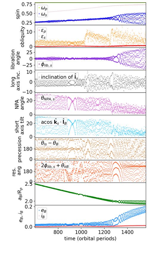
sytem is the target of the Double Asteroid Redirection                    induced torque (e.g., Kaula 1964; Goldreich 1963; Efroim-
Test (DART) mission that is one component of the AIDA                     sky and Makarov 2013)
project (Cheng et al., 2016). The DART spacecraft will                                                                 5
                                                                                                       2
                                                                                                   3 GMpert

impact the binary’s secondary fall 2022 to study the mo-                                                          R
                                                                                      τtidal     =                          k2 sin 2    (1)
mentum transfer caused by a kinetic impact. The Light                                              2 aB           aB
Italian Cubesat for Imaging of Asteroids (LICIA cube),
carried with the DART spacecraft, will take in situ obser-                where orbital semi-major axis is aB . Here k2 sin 2 is fre-
vations of the impact. Images of the surface morphology                   quency dependent and is known as a quality function. It
of the two bodies in the Didymos system will probe how                    is often approximated as k2 /Q with energy dissipation or
deformation occurs in a microgravity environment, giving                  quality factor Q and Love number k2 describing the de-
constraints on binary asteroid internal structure, forma-                 formation and dissipation in the body with mass M . See
tion and evolution mechanisms.                                            Efroimsky (2015) for discussion on the accuracy of this
                                                                          approximation.
1.1. Outline                                                                  For an incompressible homogeneous spherical elastic
                                                                          body, the Love number
    Inspired by the opportunity represented by DART and
associated missions, we examine the spin evolution of the                                                         eg
                                                                                                     k2 ∼ 0.038                          (2)
Didymos binary system. In section 1.2 we review estimates                                                         µ
for the tidal spin down time of both bodies in the system.
In section 2 we explore rotation states and evolution of a                where µ is the body’s rigidity (equal to the shear modulus
binary asteroid system using our mass/spring model sim-                   if the body is incompressible) and
ulation code (Quillen et al., 2019a,b, 2020). Our simula-
                                                                                                             GM 2
tions are similar to the soft sphere simulations described                                            eg ≡                               (3)
by Agrusa et al. (2020), except internal dissipation occurs                                                   R4
due to damping in the springs. Because we are interested                  is a measure of the body’s gravitational energy density,
in long term evolution, our simulations are carried out for               (following Equation 6 by Quillen et al. 2017 and based
more rotation periods than those by Agrusa et al. (2020).                 on Murray and Dermott 1999; Burns and Safronov 1973).
In section 2.2 we use mass-spring model viscoelastic simu-                Note that at constant density, M ∝ R3 , the energy density
lations to examine the process of secondary tidal spin down               eg ∝ R2 and Love number k2 ∝ R2 which gives a size
and tidal lock. In section 2.3 we mimic subsequent BY-                    dependent Love number similar to (but not identical to)
ORP induced migration in the binary orbital semi-major                    the weaker k2 ∝ R proposed by Goldreich and Sari (2009);
axis aB through forced migration and examine its affect on                Jacobson and Scheeres (2011).
the spin dynamics. In section 3 using triangular surface                      Using the torque of equation 1, and equation 2, we
models we explore how obliquity and non-principal axis                    estimate a spin down rate
(NPA) rotation affects estimates of the BYORP induced
                                                                                                                      6
drift rate. A summary and discussion follows in section 4.                                       GM 2 /R4

                                                                                                                 R           Mpert
                                                                                                                           GMpert
                                                                            ω̇tidal ∼ 0.14                                        .
                                                                                                   µQ            aB           R3
                                                                                                                              M
1.2. Properties of the Didymos binary system                                                                                      (4)
   In Table 1, we list properties of the Didymos binary                       A particle resting on the surface can leave due to cen-
system. We refer to the primary as Didymos and the sec-                   trifugal acceleration if the spin ω & ωbreakup with
ondary as Dimorphos. Many of the quantities in this table                                            r         r
were measured or recently reviewed by Naidu et al. (2020).                                              GM       4πGρ
                                                                                         ωbreakup ≡          =         ,          (5)
                                                                                                        R3          3
1.3. Tidal spin down rates for primary and secondary
                                                                          where ρ is the body’s mean density. If the initial spin is
    To estimate the tidal torque, we consider a uniform                   equal to the that of centrifugal breakup ωinit = ωbreakup
density spherical body that is part of binary system. The                 then
body is initially not tidally locked, so it is not in the spin
                                                                                                       23   9    s
synchronous state which is also called the 1:1 spin-orbit

                                                                                            2    M          aB 2 Q Mpert + M
resonance. The spin-down rate ω̇ and a spin down time                       tdespin ≈ Porb
                                                                                           15π Mpert        R    k2      Mpert
tdespin can be estimated from the tidally generated torque
                                                                                                                                 (6)
τtidal with ω̇tidal = τtidal /I and tdespin ∼ ω̇tidal /ωinit (e.g.,                         q
                                                                                                      a3
Peale 1977; Gladman et al. 1996) where the body’s mo-                     where Porb = 2π G(Mpert  B
                                                                                                     +M ) is the binary orbital period.
ment of inertia, I = 52 M R2 , the body’s initial spin is ωinit               Using equations 2 and 3 the spin down time is
and the body’s mass and radius are M and R.                                                  23   9              s
    The secular part of the semi-diurnal (l = 2) term in the              tdespin       M          aB 2         µQ         Mpert + M
                                                                                  ≈1                                                    .
Fourier expansion of the perturbing potential from point                    PB         Mpert        R       GM 2 /R4          Mpert
mass Mpert (the other mass in the binary), gives a tidally                                                                          (7)
                                                                      2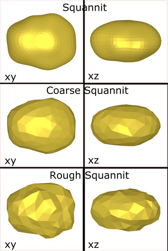
Table 1:   Didymos and Dimorphos properties
 Parameter                                    Symbol        Value                    Comments/Reference
 Binary orbital period                        PB            11.9217 ± 0.0002 hour Scheirich and Pravec (2009)
 Binary orbital semi-major axis               aB            1.19 ± 0.03 km           Naidu et al. (2020)
 Binary orbit eccentricity                    eB            < 0.03                   Scheirich and Pravec (2009)
 Didymos spin rotation period                 Pp            2.2600 ± 0.0001 hours Pravec et al. (2006)
 Didymos body diameter                        2Rp           780 ± 30 m               Naidu et al. (2020)
 Diameter or radius ratio                     Rs /Rp        0.21 ± 0.21              Scheirich and Pravec (2009)
 Semi-major axis/radius primary               aB /Rp        3.05
 Dimorphos diameter                           2Rs           164 ± 18 m               From Rp and Rs /Rp measurements
 Dimorphos spin rotation period               Ps            11.92 hours              Spin synchronous state assumed
 Total mass                                   Mp + Ms       5.37 ± 0.44 × 10¹¹ kg    Kepler’s third law
 Mass ratio                                   q = Ms /Mp 0.0093                      From ratio of radii
 Mass of Didymos                              Mp            5.32 × 10¹¹              From mass ratio
 Mass of Dimorphos                            Ms            4.95 × 10⁹               From mass ratio
                                                                       3
 Mean density of Didymos                      ρp            2.14 g/cm                From mass and radius
 Mean density of Dimorphos                    ρs            ρs = ρp                  Assumed
 Period ratio (orbit/spin primary)            PB /Pp        5.28
 Didymos body axis ratios                     ap : bp : cp  1:0.98:0.95              Based on Naidu et al. (2020)
 Didymos spin pole in ecliptic coordinates (λ, β)           (310◦ , −84◦ )           Naidu et al. (2020)
  Radii Rp , Rs are assumed to be those of the volume equivalent sphere. We refer to the primary as Didymos and the
secondary as Dimorphos. Dydimos’ body axis ratios are based on the Dynamically Equivalent Equal Volume Ellipsoid
which is an uniform density ellipsoid with the same volume and moments of inertia as the shape model by Naidu et al.
 (2020) and taken from their Table 3. Light curve observations by Pravec et al. (2006) and radar data by Naidu et al.
(2020) are consistent with the secondary being in the spin synchronous state (tidally locked). The assumption of equal
    primary and secondary densities is supported by radar observations of NEA 2000 DP107 (Margot et al., 2002).

                                  Table 2: Didymos and Dimorphous estimated properties
                                    energy density      eg,p         830 Pa
                                    energy density      eg,s         37 Pa
                                    gravity timescale   tgrav,p      1282 s
                                    breakup spin        ωbreakup,p   7.8 × 10⁻⁴ s−1

                                                           3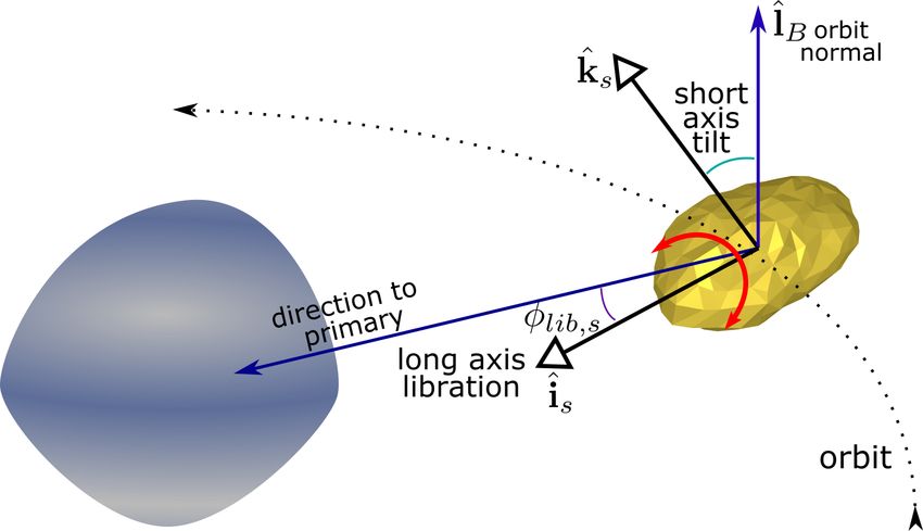
This equation can be used for either a spinning primary                          tidal drift rate is underestimated by equation 11 (Taylor
or a spinning secondary. In the case of a spinning primary                       and Margot, 2011), as we discussed in section 1.
                         32          92                r                        Constraints on asteroid internal properties based on
  tdespin,p         Mp            aB             µp Qp           Mp + Ms         tidal evolution of the orbital semi-major axis are only rel-
            ≈
     PB             Ms            Rp            GMp2 /Rp4          Ms            evant if the BYORP induced drift rate is low (e.g., Tay-
                                                                       (8)       lor and Margot 2011) or if the tidal dissipation is suffi-
                                                                                 ciently strong that the tidal torque can counter the BY-
where subscript p refers to quantities for the primary, sub-                     ORP torque (Jacobson and Scheeres, 2011). The median
script s refers to quantities for the secondary and subscript                    value for small main belt binaries (primary radius ∼ 3
B refers to quantities describing the binary mutual orbit.                       km), estimated with a collisional lifetime of ∆t = 109 yr, is
In the case of a spinning secondary                                              µp Qp ∼ 1011 Pa whereas that for small NEA binaries (with
                   3  9                  s                                 primary radius less than 1 km), estimated with a lifetime
  tdespin,s      Ms 2 aB 2            µs Qs      M p + Ms                        of ∆t = 10 Myr is µp Qp ∼ 5 × 10⁸ Pa (Taylor and Margot,
            ≈                                              .
    PB           Mp       Rs        GMs2 /Rs4       Mp                           2011). Assuming an equilibrium state between BYORP
                                                          (9)                    and tidal torque, Jacobson and Scheeres (2011) estimate
                                                                                 BQp /k2p ∼ 103 giving Qp /k2p ∼ 106 . With BYORP coef-
    Wobble damping timescales estimated from asteroid                            ficient B ∼ 10−3 this gives Qp µp ∼ 108 Pa, similar to that
light curves give an estimate for asteroid viscoelastic ma-                      estimated for NEA asteroid binaries by Taylor and Mar-
terial properties µQ ∼ 1011 Pa (Harris, 1994; Pravec et al.,                     got (2011). (Here we used equation 2 for the Love number,
                                                                                                                     2
2014). Using this value for primary and secondary we es-                         and estimated 0.038G (4π/3ρp Rp ) ∼ 102 Pa with values
timate                                                                                                         3
                                                                                 Rp = 1 km and ρp = 2 g/cm .)
                                                                                   As emphasized by Wisdom (1987), a non-round body
                               µp Qp        aB 3
  tdespin,p ≈ 2.4 × 10¹¹ yr     11
                                                                                 must tumble before entering the spin-synchronous state.
                              10 Pa      1.19 km                                 Numerical simulations show that the time for obliquity
               q −2  R −5                       − 23
                                p             ρp                                 and libration and non-principal axis rotation to damp can
            ×                                                                    substantially prolong the time it takes to reach a spin
               0.0093        390 m       2.1 g cm−3
                                                         (10)                    synchronous state with low obliquity, low free libration

                                                   3
                                                                                 and undergoing principal axis rotation (Naidu and Mar-
                              µs Qs        aB
  tdespin,s ≈ 5.8 × 10⁸ yr                                                       got, 2015; Quillen et al., 2020). Hence the long spin down
                             1011 Pa    1.19 km                                  time estimated for Dimorphos in equation 11 suggests that
               q 2  R −5                      − 32
                              s            ρs                                    Dimorphos could have spent a long period of time in a
            ×                                            (11)                    complex spin state that is nearly synchronous but has
               0.0093      82 m       2.1 g cm−3
                                                                                 non-principal axis (NPA) rotation, obliquity oscillations
using quantities measured for Didymos and Dimorphos                              and high amplitude libration. Naidu and Margot (2015)
listed in Table 1. Here q = Ms /Mp is the secondary to                           pointed out that libration amplitudes can be difficult to
primary mass ratio.                                                              detect from a light curve and epochs of chaotic tumbling
    The long primary spin-down time in Equation 10 im-                           could prolong the lifetime of a binary asteroid as BYORP
plies that tidal dissipation does not affect the primary’s                       induced drift in the tumbling state is expected to be neg-
spin. Most binaries with near circular orbits have quickly                       ligible.
spinning primaries, with periods of a few hours (Pravec
et al., 2016). On an asteroid, the reflection, absorption and
emission of solar radiative energy produces a torque that                        2. Mass/spring model simulations of an asteroid
changes the rotation rate and obliquity of a small body.                            binary
The Yarkovsky-O’Keefe-Radzievskii-Paddack (YORP) ef-                                 To explore the spin evolution of the two non-spherical
fect can account for the primary high spin rates (Ru-                            bodies in an asteroid binary, we use the mass-spring model
bincam, 2000; Scheeres, 2015; Hirabayashi et al., 2015).                         simulation code (Quillen et al., 2016a; Frouard et al., 2016;
YORP could also slow down the primary’s spin, though                             Quillen et al., 2016b, 2017, 2019a,b, 2020), that is built on
at slow spin rates, the binary system may become unsta-                          the modular N-body code rebound (Rein and Liu, 2012).
ble and disrupt leading to fewer binaries with slowly spin-                      In our code, a viscoelastic solid is approximated as a col-
ning primaries. For an illustration of an instability caus-                      lection of mass nodes that are connected by a network
ing binary disruption, see Figure 14 by Davis and Scheeres                       of springs. Springs between mass nodes are damped and
(2020).                                                                          the spring network approximates the behavior of a Kelvin-
    The timescale in equation 11 for spin down time of the                       Voigt viscoelastic solid.
secondary is longer than the estimated NEA lifetime and is                           In our previous work we only resolved a single spinning
in conflict with the large number of binary asteroids with                       body with masses and springs, though the body could be
synchronous secondaries unless the binary asteroids were                         perturbed by point masses (e.g., Quillen et al. 2017). Here
born in the main belt before they became NEAs or the
                                                                             4
Initial node distribution and spring network for each
body is chosen with the tri-axial ellipsoid random spring
model described by Frouard et al. (2016); Quillen et al.
(2016b). The confining surface used to generate the par-
2 2 2
ticles obeys xa2 + yb2 + zc2 = 1 with a, b, c equal to half the
lengths of the desired principal body axes. Particles can-
not be closer than a minimum distance dI from each other.
Since we generate the resolved bodies with only a few par-
ticles, axis ratios are more accurately computed using the
eigenvalues of the moment of inertia matrix after we gen-
erate the particle distribution. For principal moments of
q A ≥ B ≥ C, we q
inertia compute the body axis ratios as
b
a = A+C−B
A+B−C and a =
c B+C−A
A+B−C .
Figure 1: A snapshot of the mass/spring model simulation of a binary
Once the particle positions have been generated, ev-
asteroid with output shown in Figure 2. The green lines show springs
and the gray spheres show mass nodes. Both primary and secondary ery pair of particles within distance dSpr of each other
shapes are resolved with mass nodes. are connected with a single spring. The parameter dSpr
is the maximum rest length of any spring in the network.
Springs have a spring constant kSpr , giving elastic behav-
we resolve both primary and secondary in the asteroid bi- ior and a damping rate parameter γSpr giving viscous be-
nary with masses and springs. We do not include the effect havior (Frouard et al., 2016). Our simulated material is
of planets or tidal perturbations associated with the helio- compressible, so energy damping arises from both devia-
centric orbit. As we are interested in the behavior of long toric and volumetric stresses. Springs are created at the
integrations (as when we studied the obliquity of Pluto beginning of the simulation and do not grow or fail during
and Charon’s satellites, Quillen et al. 2017) rather than the simulation, so there is no plastic deformation. For nu-
details of internal tidal dissipation (Quillen et al., 2019a) merical stability, the simulation time-step must be chosen
we only use a dozen mass nodes to resolve the secondary so that it is shorter than the time it takes elastic waves to
and about a hundred mass nodes to resolve the primary. travel between nodes (Frouard et al., 2016; Quillen et al.,
The bodies are not round. Because we resolve the bod- 2016b). All mass nodes in the primary have the same
ies with individual mass nodes, we do not need to expand mass and all springs in the primary have the same spring
their gravitational perturbations in multipole terms. See constant and damping parameter. All mass nodes in the
Figure 1 for a snap shot of one of our binary simulations. secondary have the same mass and all springs in the sec-
The mass particles or nodes in both resolved spinning ondary have the same spring constant. However, the mass
bodies are subjected to three types of forces: the gravi- nodes in the primary are not the same mass as those in the
tational forces acting on every pair of mass nodes in the secondary. Similarly the spring constants of the springs in
simulation, and the elastic and damping spring forces act- the primary differ from those in the secondary.
ing only between sufficiently close particle pairs. As all
forces are applied equal and oppositely to pairs of point 2.1. Simulation output
particles and along the direction of the vector connecting
the pair, momentum and angular momentum conservation At the beginning of the simulation we store the posi-
are assured. tions of the mass nodes for both primary and secondary.
We work with mass in units of Mp , the mass of the The positions are in a coordinate system with x axis aligned
primary in the asteroid binary, distances in units of volu- with the long principal body axis and z axis aligned with
metric radius, Rvol,p , the radius of a spherical body with the short principal body axis. The position of node j
the same volume as the primary, and time in units of tgrav from the center of mass of the body in which it resides
is r0j = (rj,0
0 0
, rj,1 0
, rj,2 0
) where rj,0 is the x coordinate. The
s
3
s position of node j from the center of mass of the body in
Rvol,p 3
tgrav ≡ = . (12) which it resides at a later time during the simulation is
GMp 4πGρp rj = (rj,0 , rj,1 , rj,2 ). At each simulationP 0output we com-
pute the covariance matrix Sαβ = j rj,α rj,β using the
This timescale at the density of the primary for the Didy- current node positions and the initial node positions. The
mos system is listed in Table 2. covariance matrix is stored so that we can later compute
In our simulations, the primary and secondary are ap- a rotation describing the body orientation at each simu-
proximately the same density. Spin is given in units of lation output using the Kabsch algorithm (Kabsch, 1976;
ωbreakup = t−1
grav (see equation 5) and computed using the Berthold and Horn, 1986; Coutsias et al., 2004). At each
mean density of the primary which is 3/(4π) in our nu- simulation output the current body orientation is given by
merical units. This frequency is also listed in Table 2 for a rotation that we describe with a unit quaternion. The
the estimated density of Didymos. quaternion rotates the initial body node positions to give
5the node positions at the simulation output time. This radial velocity component, vr = drdt . The mean radius r̄
quaternion is equivalent to the unit eigenvector associ- and mean motion are estimated by smoothing the time
ated with the maximum eigenvalue of a 4x4 matrix derived series of r and nB with a Savinsky-Golay filter that has
from the covariance matrix Sαβ (Berthold and Horn, 1986; a window length of a few orbits. The epicyclic angle is
Coutsias et al., 2004). From the covariance matrix at each then θkB = arctan2((r − r̄)nB , vr ). The angles θB , θkB
simulation output we compute a quaternion at each simu- are used instead of orbital elements because a Keplerian
lation output time. We use this quaternion to compute the approximation is poor due to the non-spherical shapes of
orientation of the body’s long and short axis by rotating the primary and secondary (e.g., Renner and Sicardy 2006;
the x and z axes at each simulation output time. Agrusa et al. 2020).
At each simulation output time we compute the pri-
mary and secondary’s moment of inertia matrix from the 2.2. Simulation of secondary tidal spin down
positions of their mass nodes with respect to the body’s We carry out a simulation with simulation parame-
center of mass. The spin angular momenta for each body, ters listed in Table 3. The secondary is initially spinning
Ls , Lp , are computed from the positions and velocities of quickly and is not in a spin-orbit resonance. For this simu-
each body’s mass nodes. The spin vectors for each body, lation we set the damping parameters for the springs to be
ω s , ω p are computed from the body spin angular momen- at relatively high values so that we can see the process of
tum vectors and the inverse of their moment of inertia tidal spin down due to dissipation in the secondary. Sec-
matrices, e.g., ω s = I−1
s Ls . ondary to primary mass ratio, body axis ratios, primary
We denote the directions of the secondary’s long and spin, and binary orbital semi-major axis are intended to
short body principal axes as îs and k̂s , respectively. The be similar to those of the Didymos system. The numbers
intermediate secondary body principal axis is ĵs . The in- of mass nodes and springs in each body and ellipsoid axis
clination of the secondary’s long principal axis is the angle ratios measured from the body’s moments of inertia are
between îs and the binary orbital plane. The secondary’s listed in Table 3.
non-principal angle θN P A,s is the angle between the sec- Both bodies were initially set to be rotating about their
ondary’s short principal axis k̂s and the direction of the shortest principal axis and at zero obliquity. Here obliquity
secondary’s spin angular momentum, Ls . The secondary’s is the angle between body spin angular momentum and
short axis tilt is the angle between the secondary’s short binary orbit normal vector direction l̂B . The binary orbit
axis and the orbit normal, arccos(k̂s · l̂B ). The orbit nor- is initially in the xy plane with orbit normal l̂B = ẑ in
mal is close to the z axis during the simulation. The the z direction. We set the spin of the primary to be
secondary’s precession angle θls is the angle on the xy ωp = 0.8 ωbreakup = 0.8 t−1 grav , below the near 1 value that
plane of the secondary’s spin angular momentum vector, Didymos currently has, to ensure that self-gravity can hold
θls = arctan2(Lsy , Lsx ) where Ls = (Lsx , Lsy , Lsz ). The the primary together while keeping the springs under slight
obliquities for primary and secondary s , p are the angle compression. As springs do not dissolve in our simulation,
between body spin angular momentum and orbital normal a rapidly spinning body near rotational breakup would
l̂B . The secondary libration angle φlib,s is that between unphysically put the springs under tension. The secondary
the secondary’s long principal body axis, projected onto is initially at ωs = 0.5 ωbreakup .
the orbital plane, and the vector connecting primary and The binary orbit was begun at low orbital eccentric-
secondary centers of mass. ity. The initial orbit eccentricity eB is not exactly zero
The binary orbit normal l̂B direction is computed us- because we compute it without taking into account the
ing the body center of mass positions and velocities. The non-spherical mass distributions of primary or secondary
orbital semi-major axis aB , eccentricity eB and inclination (for discussion on this issue see Agrusa et al. 2020).
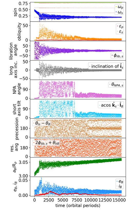
iB are computed from the positions and velocities of the In Figure 2, we plot primary and secondary spin in
primary and secondary center of mass and assuming Ke- units of t−1
grav , obliquity, secondary libration angle, orbital
plerian motion (we assume point masses so the extended semi-major axis, eccentricity and inclination as a function
mass distributions are not taken into account). The or- of time. The horizontal axis shows time in units of the
bital inclination is zero if the binary orbit lies in the xy initial binary orbital period, PB . All angles are in degrees
plane. We measure the angle of the secondary in its orbit, except for the orbital inclination iB which is in radians.
θB , from the vector between the two body center of mass In this figure we also plot the secondary’s long axis incli-
positions, r, projected into the xy plane. As orbital in- nation angle, non-principal axis angle θN P A,s , short axis
clination and eccentricity are low, θB = arctan2(ry , rx ) is tilt angle, and resonant angles associated with precession
approximately equal to the binary’s mean longitude, λB . and libration.
Using an epicyclic approximation we measure an epicylic In the top panel of Figure 2, we plot both primary
angle θkB describing radial oscillations of the orbit. The and secondary spins. Dotted lines show the locations of
epicyclic angle is computed from the vector between sec- spin-orbit resonances where the spin is equal to the binary
ondary and primary, the radius r = |r, the mean value orbit mean motion ω = nB /j divided by integer j. The
of the radius, r̄, the orbital mean motion nB , and the secondary enters the 1:1 spin-orbit resonance at about t ≈
1000 PB at which time the libration angle φlib,s begins to
6Figure 3: An illustration of the non-principal axis rotation state of
the secondary for the simulation shown in Figure 2 after the sec-
ondary has entered the 1:1 spin-orbit resonance. The secondary’s
long axis (shown with direction îs ) remains aligned along the direc-
tion to the primary and this maintains a low libration angle φlib,s .
However, the secondary’s short axis, with direction k̂s , can rotate
as shown with red arrow. The secondary can slowly rotate about
its long axis without leaving the 1:1 spin-orbit resonance. The short
axis tilt angle is the angle between k̂s and the binary orbit normal
l̂B . The short axis can rock back and forth, as shown by the red
arrow, due to non-principal axis rotation. Replacing the secondary
with an airplane that has nose pointing to the secondary, long axis
libration is equivalent to yaw, short axis tilt is equivalent to roll and
variations in the long axis inclination are equivalent to pitch.
librate about 0. Simultaneously, the secondary’s obliquity
jumps to about s ∼ 40◦ and non-principal axis rotation is
excited. The non-principal axis rotation is reflected in the
large range exhibited by the short axis tilt angle. A smaller
jump in obliquity occurs at about t ∼ 400 PB where the
2:1 spin-orbit resonance (where ωs ≈ 2nB ) is crossed.
The simulation shown in Figure 2 illustrates that the
spin-down rate of the secondary (shown in the top panel) is
faster than the obliquity and non-principal axis damping
rate. Past a time of about 1000 orbit periods, the sec-
ondary spin rate on average is consistent with being in the
1:1 spin-orbit resonance, with secondary spin rate equal to
the binary orbit mean motion ωs ∼ nB . Long after (104
Figure 2: Simulation of a tidally evolving asteroid binary. Both
orbit periods after) the secondary enters the 1:1 spin-orbit
primary and secondary are extended non-spherical bodies. The pa-
rameters for this simulation are listed in Table 3 and a simulation resonance, its obliquity and non-principal axis rotation an-
snap shot is shown in Figure 1. The top panel shows primary and gle θN P A,s remain high and vary chaotically. Similar long
secondary spin rates in units of t−1 grav . The second panel from the lasting obliquity and non-principal axis angle variations
top shows primary and secondary obliquity (which is the angle be-
tween spin angular momentum and orbit normal). The third panel
were seen in simulations of tidally evolving Phobos and
from top shows the secondary libration angle, φlib,s . In the middle Deimos (Quillen et al., 2020). We confirm the findings of
panels, we show the inclination of the secondary’s long body axis Naidu and Margot (2015) who similarly emphasized that
with respect to the orbital plane, the secondary’s non-principal axis chaotic non-principal axis rotation of the secondary could
angle θN P A , the tilt of the secondary’s short axis with respect to the
orbit normal acos(k̂ · l̂B ), a resonant angle associated with preces-
be long-lived in binary asteroid systems.
sion and a resonant angle associated with libration. The second from The nature of the secondary’s non-principal axis ro-
bottom panel shows the binary orbit semi-major axis in units of the tation state in the simulation shown in Figure 2 is illus-
primary’s radius, aB /Rp . The bottom panel shows binary orbital trated in Figure 3. The secondary’s long body axis re-
eccentricity eB and inclination iB . Angles are in degrees except for
the binary orbit inclination in the bottom panel which is in radians. mains aligned with the direction to the primary giving it a
Time is in units of binary’s initial orbital period. This simulation low libration angle that oscillates about zero. Meanwhile
illustrates that the spin-down rate of the secondary as it approaches the short axis of the secondary can rotate. The body can
the spin synchronous state (shown in the top panel at early times) rotate about its long axis without significantly increasing
is faster than the obliquity and non-principal axis rotation damping
rate at later times. the libration angle. The secondary lies in the 1:1 spin-orbit
resonance but also exhibits significant non-principal axis
7rotation. The light curve of such a secondary might ap- 100 times longer than the spin down time, as did reso-
pear to reside in a low obliquity and tidally locked princi- nant non-principal axis rotation states seen in simulations
pal axis rotation state. It might be difficult to differentiate of Deimos; Quillen et al. 2020). In future, the theoreti-
between a principal axis rotation state and a non-principal cal framework developed by Boué and Laskar (2009) for
axis rotation state if the libration angle φlib,s remains low binary systems might be applied to better identify and
in both states. create a model for this NPA rotation resonance.
In a frame synchronous with the orbit and replacing We explored simulations similar to that shown in Fig-
the secondary with a plane that has nose pointing to the ure 2 at larger orbital semi-major axis with a larger sec-
secondary, long axis libration is equivalent to yaw, short ondary to primary mass ratio (similar to that of the binary
axis tilt is equivalent to roll and variations in the long axis system Binary Near-Earth Asteroid (66391) 1999 KW4
inclination are equivalent to pitch. now known as Moshup) and saw similar behavior to that
Figure 2 shows that the time to damp the non-principal described here. We also explored similar simulations with
axis rotation and obliquity is longer than the time it takes different axis ratios for the secondary and also saw similar
for the secondary to spin down and enter the spin syn- behavior.
chronous state. Fitting time dependent exponentially de-
creasing functions to smoothed secondary spin and obliq- 2.3. Simulations of inward migration
uity arrays, we find that the damping time is about 5 times YORP and BYORP effect torques cause slow evolu-
longer for obliquity after reaching the 1:1 spin-orbit reso- tion so they can be considered adiabatic. BYORP effect
nance than for spin prior to reaching the resonance. torque could cause the binary orbital semi-major axis to
As discussed in section 1.3, the time for the secondary drift either outward or inward (Ćuk and Burns, 2005). We
to spin down could be similar to the lifetime of NEA as- explore whether obliquity and non-principal axis rotation
teroids. With a value considered typical of main belt as- can be excited during orbital migration. We carry out a
teroids, the tidal spin down time for Dimorphos exceeds simulation that forces the binary orbital semi-major axis
the NEA lifetime. If binary asteroid secondaries are pre- to shrink with a drift rate ȧB = −10−5 Rp /tg . Migration
dominantly in principal axis rotation states, then much is forced by perturbing the center of mass velocities us-
lower values of µQ would be required to account for their ing the procedure described by Beaugé et al. (2006) and
synchronous rotation. The even longer time require for which we used previously to force outward migration of
non-principal axis rotation damping exacerbates the diffi- Charon when studying the obliquity evolution of Pluto
culty reconciling the estimates for µQ in binary and single and Charon’s minor satellites (Quillen et al., 2017). Our
asteroids. Alternatively, the asteroid binary secondaries migration simulation uses the last output of the tidal spin
could commonly be in complex rotation states with non- down simulation (shown in Figure 2) as its initial condi-
principal axis rotation. They could still reside in the 1:1 tions. Thus its parameters are the same as those listed in
spin-orbit resonance while exhibiting non-principal axis ro- Table 3 except that we set the spring damping constants
tation, as seen in our simulation shown in Figure 2. If to 0.01 so as to reduce tidal dissipation. The secondary be-
binary asteroid secondaries are commonly found in non- gins in the 1:1 spin synchronous state but with some NPA
principal axis rotation states then their tidal dissipation rotation. The migration simulation was run until the bi-
rate cannot be extremely high. Constraints on secondary nary disrupted at t ∼ 1600 PB . The simulation is shown
rotation state may improve upon tidal based estimated for in Figure 4 which has panels similar to those of Figure 2.
their material properties. We restricted the time shown in the Figure to make it eas-
In Figure 2, in the panel labeled ‘precession’ (fourth ier to see variations in angles and other quantities prior to
from bottom), we show a resonant angle θls − θB which the short period of instability that led to its breakup.
is the secondary spin angular momentum direction pro- Figure 4 shows two obliquity jumps, one at t ∼ 1070 PB
jected onto the orbital plane as seen in the frame rotating and the other at t ∼ 1300 PB . The first jump in obliquity
with the secondary in its orbit. At t ∼ 9500 PB this reso- occurs when the precession angle θls −θB ceases to be near
nant angle is mostly near zero and 180◦ and at the same zero and 180◦ and spends more time near 90◦ and 270◦ . At
time there is a jump in the secondary’s non-principal axis the same time the secondary’s long axis is tilted out of the
angle θN P A,s . The distribution of θls − θB suggests that orbital plane giving oscillations in the long axis inclination
the short axis tilts back and forth with an oscillation pe- angle. The body’s long axis tilts above and below the
riod that is twice the binary orbit period. The secondary’s orbital plane with an oscillation period that is equal to 2
spin angular momentum Ls is often aligned with the di- binary orbit rotation periods. In a frame rotating with the
rection between secondary and primary. At the same time secondary in its orbit, the secondary shifts from rotating
the secondary’s short axis, when projected onto the xy- about its long axis (and tilting its short axis w.r.t to the
plane, spends time at angle ±90◦ . The secondary’s short orbit normal) to rotating about its intermediate axis and
axis periodically rocks back and forth about the orbit nor- giving variations in the long axis inclination.
mal because of rotation about its long axis. The jump in The second jump in obliquity at t ∼ 1300PB is associ-
the non-principal axis angle θN P A,s suggests that it is a ated with an increase in the libration angle and orbital ec-
resonant state, so it could last a really long time (10 to centricity. This second jump is also associated with a tran-
8Table 3: Viscoelastic Mass/Spring Model Simulation Parameters for Tidal spin down
Description Symbol Quantity
Total integration time tmax 5 × 105 = 15400 PB
Time step dt 0.002
Initial orbital semi-major axis aB 3.0
Description Symbols For Primary For Secondary
Mass Mp , Ms 1 0.01
Radius equiv. volume sphere Rvol 1 0.22
Initial spin ωinit 0.8 0.5
Minimum interparticle distances dI 0.27 0.14
Maximum spring length/dI dSpr /dI 2.4 2.3
Spring constants kSpr 0.20 0.03
Spring damping parameters γSpr 1 30
Body axis ratios a:b:c 1.0:0.958:0.881 1.0:0.773:0.698
Number of particles N 165 18
Number of springs NSpr 1950 113
Axis ratios are those derived from the principal axis moments of inertia computed from the generated particle
positions. Time is given in units of tgrav . Distances are in units of Rp , the primary’s volume equivalent radius. Spin
rates are in units of the break up spin rate ωbreakup or equivalently t−1grav .
sition in the behavior or the resonant angle 2φlib,s + θkB . The spin state of the secondary was unaffected until the
Prior to the second transition, this angle oscillates and af- primary spin reached the spin/spin resonance ωp ∼ 2ωs
terwards it librates about 270◦ . This angle corresponds which caused the binary to disrupt. Only when the pri-
to the body rotating twice (in the frame of orbital rota- mary spin was low, did we see evidence for spin-spin reso-
tion) per epicyclic period. This resonance is similar to a nant coupling. In this setting spin/spin resonant coupling
Lindblad resonance and it is strong enough to increase the (Seligman and Batygin, 2021) could be important.
orbital eccentricity until the binary disrupts. We suspect We explored a simulation similar to that shown in Fig-
the disruption mechanism is the same as shown in Figure ure 4 except the secondary migrated outward (instead of
14 by Davis and Scheeres (2020). inward) from aB /Rp ≈ 2 to 4 at a drift rate ȧB = 5.0 ×
Because the primary spin was unaffected during the 10−6 . This simulation showed a similar obliquity jump
two obliquity transitions in the migration simulation, we at aB /Rp ∼ 2.1 as the first transition in Figure 4. This
infer that spin/spin resonant coupling (Seligman and Baty- implies that the resonance that excited the long axis in-
gin, 2021) between the two bodies was not a contribut- clination is sensitive to the binary period. Otherwise this
ing factor. Rotation of a torque free triaxial body can be simulation was dull. After that transition, we did not see
described in terms of precession and nutation (Boué and obliquity or non-principal axis excitation. Perhaps simu-
Laskar, 2009). We tentatively associate the first obliquity lations that migrate outward more slowly (adiabatically)
transition with nutation excitation. The precession and would reveal weaker resonant behavior.
nutation frequencies are sensitive to more than one canoni-
cal variable, but perhaps in future they could be calculated 3. Implications for BYORP drift
using the formalism developed by Boué and Laskar (2009)
and the location of resonances associated with them could In section 2.2 our tidal spin down simulation showed
be predicted. that secondary obliquity and non-principal axis excitation
The migration simulation shown in Figure 4 illustrates can be long-lived within the 1:1 spin-orbit resonance. In
that if the system migrates inward via BYORP, non-principal section 2.3 our migration simulation showed that obliquity,
axis rotation can be excited due to spin-orbit resonances long axis inclination and libration can be excited if the
that involve obliquity, libration, and non-principal axis ro- binary semi-major axis drifts inward due to BYORP. In
tation. Thus even if tidal dissipation is strong enough to this section we explore effect of non-principal axis rotation
damp the secondary’s obliquity and non-principal axis ro- on the BYORP drift rate for a secondary that is within
tation, inward migration could re-excite the secondary’s the 1:1 spin-orbit resonance.
rotation state. Prior calculations of the BYORP affect (Ćuk and Burns,
We also explored a simulation that forced the primary 2005; McMahon and Scheeres, 2010; Steinberg and Sari,
to spin down, as might occur due to the YORP effect. The 2011; Scheirich et al., 2021) assume that the secondary
primary spin drift rate used was ω̇p = −2 × 10⁵ t−2g and as is tidally locked (in the 1:1 spin synchronous state), un-
in our migration simulation, initial conditions were the end dergoes principal axis rotation, is at zero obliquity and
state of the tidal spin down simulation shown in Figure 2. lacks free libration. To estimate the role of non-principal
9axis rotation in affecting the BYORP induced drift rate
we compute the BYORP torque on the binary orbit us-
ing different secondary shape models that are comprised
of triangular surface meshes.
The shapes of the secondaries in most binary systems
are not well characterized. An exception is with the Bi-
nary Near-Earth Asteroid (66391) 1999 KW4, with pri-
mary known as Moshup and secondary known as Squan-
nit. Squannit’s shape model was derived by Ostro et al.
(2006) and a BYORP generated drift rate was computed
with this shape model by Scheirich et al. (2021). We use
the same Squannit shape model to compare our BYORP
drift rate estimates to that computed by Scheirich et al.
(2021).
To estimate the torque from BYORP we neglect sur-
face thermal inertia, following Rubincam (2000), so that
thermal radiation is re-emitted with no time lag. The re-
flected and thermally radiated components are assumed
to be Lambertian so they are emitted with flux parallel
to the local surface normal. We ignore heat conduction
and neglect shadows on the day-lit side. We ignore vari-
ations of albedo or emissivity on the surface. Secondary
intersections of re-radiated energy are ignored.
The asteroid surface is described with a closed triangu-
lar oriented vertex-face mesh, similar to the calculations
by Scheeres (2007); McMahon and Scheeres (2010); Stein-
berg and Sari (2011). We index each triangular facet with
an integer i. The i-th facet has area Si , and unit nor-
mal n̂i . The radiation force on the i-th triangular facet is
computed as
(
− 23 Fc Si (n̂i · ŝ )n̂i if n̂i · ŝ > 0
Fi = , (13)
0 otherwise
where F is the solar radiation flux and c is the speed of
light. The direction of the Sun is given by unit vector ŝ .
The factor of 2/3 is consistent with Lambertian reflectance
and emission. Facets on the day side have n̂i · ŝ > 0
and we assume that only these contribute to the radiation
force. In terms of the radial distance rh from the binary
to the Sun, F ≡ Pr2 where radiation pressure constant
h
Figure 4: A binary asteroid simulation that exhibits forced inward L
migration. The initial conditions for this simulation are given by P ≡ = 1017 kg m s−2 (14)
the last output of the simulation shown in Figure 2. The panels 4πc
of this figure are similar to those of Figure 2. Time is given in
orbital periods from the beginning of the simulation. This simulation and where L is the solar luminosity.
illustrates that secondary obliquity and non-principal axis rotation The torque affecting the binary orbit from a single facet
can be excited during inward orbital migration. At t ∼ 1070 PB the is
obliquity is excited, the long axis is tilted out of the orbital plane
and the resonant angle θls − θB ceases spending time at 0 and 180◦ .
(
At t ∼ 1300 PB a libration resonance is excited with resonant angle
− 32 Fc Si (n̂i · ŝ )(aB × n̂i ) if n̂i · ŝ > 0
τ i,B = ,
2φlib +θkB . The orbital eccentricity increases and the binary disrupts 0 otherwise
at t ∼ 1600 PB . This figure shows that obliquity and non-principal (15)
axis rotation can be excited in the secondary via induced migration.
where aB is the secondary’s radial vector from the binary
center of mass. We neglect the distance of the facet cen-
troids from the secondary center of mass when computing
the radiative torques.
10The torque affecting the binary orbit is the sum of the The three shape models are an icosphere, a coarse version
torques from each facet. This torque is averaged over dif- of the Squannit shape model by Ostro et al. (2006) and
ferent binary positions in its orbit around the Sun, affect- a perturbed version of the same Squannit shape model.
ing the direction of s , and over the different positions in With the Squannit shape model by Ostro et al. (2006),
the binary mutual orbit and spin rotation of the secondary, Scheirich et al. (2021) computed a BYORP B-coefficient
of B = 2.082 × 10⁻² for the Moshup/Squannit binary sys-
1 T
Z
tem. To test our BYORP B-coefficient computation, we
X
τ BY = dt τ i,B . (16)
T 0 i
compare our computed B-coefficient to that computed by
Scheirich et al. (2021).
To represent this average, time T significantly exceeds bi- The icosphere is an icosahedron that is subdivided twice.
nary and heliocentric orbit periods. In practice we sum Each triangular face of the icosahedron is divided into 4
over different orbital phases to compute the average. The triangular faces and then each of them is divided into 4
average can also be done by integrating over the mean triangular faces giving a total of 320 triangular faces. The
anomaly Mh of the binary in its heliocentric orbit and the vertex positions are then corrected so they have distance
mean anomaly of the binary orbit MB 1 from the origin.
Z 2π Z 2π X The Squannit shape model by Ostro et al. (2006) con-
τ BY = dMh dMB τ i,B . (17) tains 2292 faces is shown with xy and yz plane views in
0 0 i the top two panels of Figure 5. The red bounding squares
in this Figure have a size of 3 in units of the radius of a
If l̂B is the binary orbit normal then the mutual semi- volume-equivalent sphere. To speed up our BYORP calcu-
major axis drift rate is lation we compute the BYORP drift rate for a similar but
coarser triangular surface mesh with fewer faces. We re-
2τ BY · l̂B duce the face number by merging short edges that are less
ȧB = . (18)
Ms nB aB than a specified length. We adjusted the specified mini-
BYORP is often described in terms of a dimensionless mum edge length to give a triangular surface mesh with
number (e.g., McMahon and Scheeres 2010). By summing about 300 faces. The coarser version of the Squannit shape
over different orientations and face model facets, we cal- model with 302 faces is shown in the middle panels of 5.
culate the dimensionless number We checked that the results of our BYORP B-coefficient
calculations are not sensitive to the number of faces used
c
BBY ≡ (τ BY · l̂B ) . (19) in our model (coefficients were less than a few percent dif-
F Rs2 aB ferent than those computed with a surface mesh that has
This is equivalent to letting aB = Rs = F /c = 1. For a twice the number of faces).
binary in a non-circular heliocentric orbit, averaging of the To create a rougher version of the Squannit shape model
solar flux would give F̄ = 2 √P 2 where ah and eh are we perturbed each vertex of the coarse Squannit 302 face
ah 1−eh shape model by adding random values to the x, y and z
the binary orbit’s heliocentric semi-major axis and eccen- coordinates of each vertex. The random values are taken
tricity. With our dimensionless number, BBY , equations from a uniform distribution spanning [−∆, ∆] where ∆ =
18 and 19 give 0.05 in units of the volume-equivalent sphere. The per-
2P Rs2 turbed 302 face Squannit shape model is shown in bottom
ȧB = p gBY . (20) two panels of Figure 5. The perturbations to the vertices
a2h 1 − e2h Ms nB
make it rougher than the other original and coarse Squan-
We compare our expression to equation 3 by Scheirich et al. nit shape models.
(2021)
3.2. BYORP B-coefficients computed with randomly cho-
2 sen short axis tilt angles
2P Rmean
ȧB = B. (21)
Using the three shape models described in section 3.1,
p
a2h 1 − e2h Ms nB
we numerically compute BYORP B-coefficients in two set-
Comparison between this equation and equation 20 shows tings. In our first set of calculations, we compute B-
that our dimensionless BBY parameter of equation 19 is coefficients assuming a circular binary orbit and choosing
equivalent to the dimensionless BYORP B parameter in- orientations for the secondary at different positions in the
troduced by McMahon and Scheeres (2010). Our parame- orbit. In our second set of calculations (section 3.3), we
ter BBY = πfBY where fBY is the dimensionless parame- use the secondary orientations measured directly from our
ter computed by Steinberg and Sari (2011). simulations to compute the B-coefficients.
In our mass-spring model simulations described in sec-
3.1. Shape models tion 2, non-principal axis rotation of the secondary was
To explore how BYORP depends on surface shape we present at low libration angle and was characterized by
use 3 shape models that are triangular surface meshes. rotation about the secondary’s long axis. The secondary’s
11long axis remains aligned with the direction to the pri-
mary, corresponding to φlib,s ≈ 0, however the short axis
can tilt away from the orbit normal. We described this
rotation as the short axis tilt and it is measured from
the angle between the body short axis and the orbit nor-
mal. We assume that the secondary angular rotation rate
ωs = nB is equal to the binary orbit mean motion. This
condition places the secondary in the 1:1 spin synchronous
resonance. We orient the secondary so that its long axis re-
mains in the orbital plane and points directly toward the
primary so that the libration angle remains at zero. At
each binary orbit orientation, the secondary’s short axis
orientation is randomly chosen using a uniform distribu-
tion so that the angle between the short axis and the orbit
normal ranges from 0 to a maximum of θmaxtilt . Specif-
ically, after rotating the secondary so that its long axis
is pointed toward the primary, the secondary is rotated
about its long axis by an angle chosen from a uniform dis-
tribution within {−θmaxtilt , θmaxtilt }.
We assume a zero inclination circular orbit for the bi-
nary (about the Sun) and a circular mutual binary orbit.
To numerically calculate the BYORP B-coefficient we first
Figure 5: Triangular surface mesh shape model for Squannit by Ostro average over the Sun’s possible directions using 36 equally
et al. (2006) is shown in the top two panels. The xy plane is viewed
on the left and the xz plane is viewed on the right. This shape model
spaced solar angles. Then we average over the binary or-
has 2292 faces. The middle two panels shows a coarser version of the bit using 144 equally spaced binary orbit orientations. In
same shape model with 302 faces. The bottom two panels show a each of these 144 possible orientations the short axis tilt
model that is similar to the coarse one, but each vertex position is randomly chosen.
has been perturbed in a random direction to increase the surface
roughness. The red bounding squares have a length of 3 in units of The BYORP B-coefficients computed using the three
the radius of the volume equivalent sphere. shape models shown in Figure 5 and with randomly chosen
short axis tilt angles are shown in Figure 6 as a function
θmaxtilt . The green circles show that the B-coefficient com-
puted for the icosphere is zero, as expected. The coarse
Squannit face model, shown with red squares, gives a BY-
ORP B-coefficient of BBY = 0.02 for θmaxtilt = 0 and
this agrees with the value computed by Scheirich et al.
(2021) for Squannit that is shown with a black circle. For
both Squannit and rough Squannit shape models, the BY-
ORP B-coefficient drops to zero at a maximum tilt angle
of about θmaxtilt ∼ 60◦ . This gives a quantitative estimate
for how much non-principal axis rotation within the 1:1
spin-orbit resonance is required to reduce BYORP drift.
The rough or perturbed Squannit shape model gives
lower values of the BYORP B-coefficient than the Squan-
nit shape model. This is opposite to the expected trend.
Usually rougher surface models have higher YORP and
BYORP coefficients Steinberg and Sari (2011). By com-
Figure 6: BYORP B-coefficients computed using two Squannit sec- puting BYORP B-coefficients for perturbed ellipsoids we
ondary shape models shown in the bottom four panels of Figure 5, confirmed that rougher surfaces tend to have larger B-
as a function of the maximum tilt angle of the body’s short axis
from the orbit normal. The body tilt is randomly chosen at each
coefficients. The specific shape of the Squannit shape
binary orbit orientation angle used in the torque averaging compu- model must be responsible for its high B-coefficient. The
tation. The black circle is the B-coefficient computed by Scheirich ratio of B-coefficients for Squannit and perturbed Squannit
et al. (2021) based on the Squannit model by Ostro et al. (2006). shape models we computed at θmaxtilt = 0 is less than 2. In
The green circles are computed for an icosphere. The red squares
show the coarse Squannit shape model with 302 faces. The brown
the Moshup/Squannit system, Scheirich et al. (2021) mea-
crosses show a perturbed or rough Squannit shape model, also with sured a drift rate about 8 times lower than predicted. A
302 faces. The BYORP B-coefficient reverses sign when the short rougher surface for Squannit does not give a large enough
angle tilts by more than about 60◦ . difference in the B-coefficient to fully account for its low
measured B-coefficient (assuming principal axis rotation).
12Figure 7: BYORP-B coefficient is computed using secondary and bi- Figure 8: Similar to Figure 7 except the BYORP B coefficient is
nary orientations from the tidal spin-down simulation shown in Fig- computed using the migration simulation shown in Figure 4. As the
ure 2 and is shown in the top panel as a function of time in orbital non-principal axis rotation angle drops, the BYORP B-coefficients
periods. The B-coefficients were computed using our three shape for the Squannit shape models increase.
models. The red squares are the coarse Squannit shape model, the
brown pluses are the perturbed (or rougher) Squannit shape model.
The green circles show an icosphere shape model. The icosphere has 18 solar positions were used to compute an average BY-
a B-coefficient of zero, as expected. The secondary’s non-principal
axis angle θN P A,s is shown in the bottom panel. The BYORP B- ORP torque. 100 consecutive simulation outputs, span-
coefficients for the Squannit shape models frequently reverse in sign. ning about 6 binary orbit periods, were then combined
Only after the NPA angle has dropped below 45◦ near the end of for an average of the BYORP induced torque at a par-
the simulation does the BYORP B-coefficient remain positive. The ticular moment during the simulation. We note that the
rougher Squannit shape model has B-coefficients similar to but lower
amplitude than the coarse Squannit shape model. Both Squannit axis ratios of the Squannit shape model (bs /as = 0.762,
shape modes have BYORP B-coefficients lower than predicted for cs /as = 0.576; Ostro et al. 2006) are similar to but not ex-
a tidally locked body undergoing principal axis rotation, at zero actly the same as those of the secondary in the simulation
obliquity and with no free libration. The conventionally predicted
(0.773, 0.698).
B-coefficients are 0.02 for the coarse Squannit model and 0.014 for
the rough Squannit model. This figure shows that long-lived non- To check our numerical routines we ran a short simu-
principal axis rotation within the 1:1 spin-orbit resonance can cause a lation of a secondary in the spin synchronous state, zero
reduction in the amplitude of the BYORP B-coefficient and reversals obliquity and in a principal axis rotation rate. We mea-
in the direction of BYORP effect drift.
sured the BYORP B-coefficient in this short simulation.
The measured B-coefficient values for each shape model
In contrast, the BYORP B-coefficient can be negligible if were consistent with those computed at θmaxtilt = 0, and
there is non-principal axis rotation with θmaxtillt ∼ 60◦ . shown in Figure 6, for the same shape models, as expected.
The B-coefficient computed for the coarse Squannit shape
3.3. BYORP B-coefficients computed using the mass-spring model again agreed with that computed by Scheirich et al.
model numerical simulations (2021), BBY ≈ 0.02.
We find the secondary orientation at each simulation Figure 7 shows the BYORP B-coefficients computed
output in our mass-spring model simulations. We use the for our three shape models from the tidal spin-down simu-
vector between secondary and primary, binary orbit nor- lation shown in Figure 2 as a function of time and Figure 8
mal and body orientation at each simulation output to similarly shows the BYORP B-coefficients but computed
compute the BYORP B-coefficient for three shape mod- for the migration simulation shown in Figure 4. In these
els, two of which are shown in Figure 5. figures, green circles refer to the icosphere shape model,
The secondary orientation (computed with a quater- red squares refer to the 302 face coarse Squannit shape
nion from a simulation output as described in section 2.1) model and brown pluses refer to the rougher Squannit
was used to rotate the shape model vertices. The rotated shape model. In both figures the top panels show the B-
shape model vertices, face normals and face areas were coefficients and the bottom panels show the non-principal
then used to compute the radiative torque on each facet axis angle θN P A,s .
using binary orientation vector and orbit normal from the Figure 7 shows that the BYORP B-coefficients are lower
concurrent simulation output. At each simulation output, than those computed for principal axis rotation state (BBY ≈
13You can also read