Advanced Modeling and Simulation of Rockfall Attenuator Barriers Via Partitioned DEM-FEM Coupling
←
→
Page content transcription
If your browser does not render page correctly, please read the page content below
ORIGINAL RESEARCH
                                                                                                                                               published: 14 June 2021
                                                                                                                                        doi: 10.3389/fbuil.2021.659382

                                            Advanced Modeling and Simulation of
                                            Rockfall Attenuator Barriers Via
                                            Partitioned DEM-FEM Coupling
                                            Klaus Bernd Sautter 1*, Helene Hofmann 2, Corinna Wendeler 3, Peter Wilson 4,
                                            Philipp Bucher 1, Kai-Uwe Bletzinger 1 and Roland Wüchner 1,5
                                            1
                                             Chair of Structural Analysis, Technical University of Munich, Munich, Germany, 2Geobrugg AG, Romanshorn, Switzerland,
                                            3
                                             Appenzell Ausserrhoden, Department of Construction and Economics, Civil Engineering Office, Hydraulic Engineering, Herisau,
                                            Switzerland, 4School of Civil Engineering, The University of Queensland, Brisbane, QLD, Australia, 5International Center for
                                            Numerical Methods in Engineering, Technical University of Catalonia, Barcelona, Spain

                                            Attenuator barriers, in contrast to conventional safety nets, tend to smoothly guide
                                            impacting rocks instead of absorbing large amounts of strain energy arresting them. It
                                            has been shown that the rock’s rotation plays an important role in the bearing capacity of
                           Edited by:
                                            these systems. Although experimental tests have to be conducted to gain a detailed insight
                 Stefano de Miranda,        into the behavior of both the structures and the rock itself, these tests are usually costly,
           University of Bologna, Italy     time-consuming, and offer limited generalizability to other structure/environment
                       Reviewed by:         combinations. Thus, in order to support the engineer’s design decision, reinforce test
                      Alessio Mentani,
           University of Bologna, Italy     results and confidently predict barrier performance beyond experimental configurations
                      Rossana Dimitri,      this work describes an appropriate numerical modeling and simulation method of this
           University of Salento, Italy
                      Shuji Moriguchi,
                                            coupled problem. For this purpose, the Discrete Element Method (DEM) and the Finite
            Tohoku University, Japan        Element Method (FEM) are coupled in an open-source multi-physics code. In order to
                             Lei Zhao,      flexibly model rocks of any shape, sphere clusters are used which employ simple and
       Southwest Jiaotong University,
                                 China      efficient contact algorithms despite arbitrarily complicated shapes. A general summary of
                  *Correspondence:          the FEM formulation is presented as well as detailed derivations of finite elements
                 Klaus Bernd Sautter        particularly pertinent to rockfall simulations. The presented modeling and coupling
                klaus.sautter@tum.de
                                            method is validated against experimental testing conducted by the company
                  Specialty section:
                                            Geobrugg. Good agreement is achieved between the simulated and experimental
       This article was submitted to        results, demonstrating the successful practical application of the proposed method.
 Computational Methods in Structural
                         Engineering,       Keywords: DEM, FEM, rockfall, impact, cluster, experiment, particles, coupling
             a section of the journal
      Frontiers in Built Environment
         Received: 27 January 2021          1 INTRODUCTION
           Accepted: 18 May 2021
          Published: 14 June 2021           Rock impact is an exceptional load case due to many factors. The shape, the density and the motion
                              Citation:     process itself of the impacting object can be arbitrary and difficult to predict. The additional
Sautter KB, Hofmann H, Wendeler C,          dynamics and arbitrariness of the impact point make it impossible to determine a generally valid load
  Wilson P, Bucher P, Bletzinger K-U        assumption formula. This raises the question of how to design protective structures for such load
   and Wüchner R (2021) Advanced
 Modeling and Simulation of Rockfall
   Attenuator Barriers Via Partitioned
                  DEM-FEM Coupling.         Abbreviations: DEM, Discrete Element Method; FEM, Finite Element Method; HM + D, Hertz-Mindlin Spring-Dashpot
       Front. Built Environ. 7:659382.      MPM, Material Point Method; PFEM, Particle Finite Element Method; SPH, Smoothed-Particle Hydrodynamics; Bold letters
      doi: 10.3389/fbuil.2021.659382        indicate vectors and tensors.

Frontiers in Built Environment | www.frontiersin.org                               1                                             June 2021 | Volume 7 | Article 659382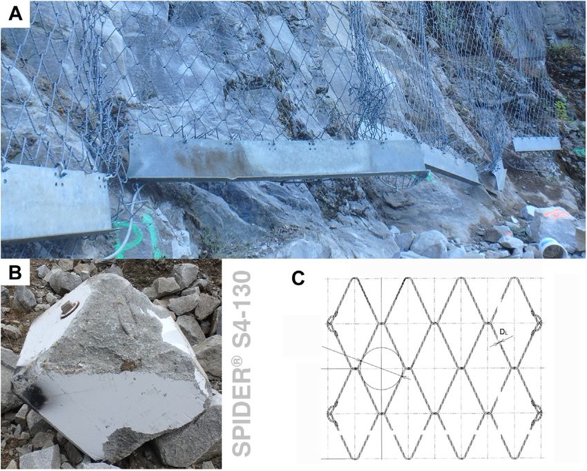
Sautter et al.                                                                                                           Advanced Simulation of Attenuator Barriers

  FIGURE 1 | All photos are property of Geobrugg (www.geobrugg.com). (A) Banya railway rockfall protection. (B) Monserrate walking path. (C) Kaikoura State
  Highway, Attenuator barrier. (D) Attenuator barrier after impact. Photo of the experiment discussed in section 3.

cases. During rock impact events, protective structures are                          accelerations and angular velocities. Since the exact orientation
generally engineered to deform greatly, which reduces peak                           of the rock at impact cannot be determined precisely, these data
system decelerations and safely dissipates large amounts of                          are only compared in terms of their general trends instead of
energy.                                                                              exact values (see section 5.2). In order to better understand the
   In order to allow the protective structure to undergo large                       interaction between impacting objects and highly flexible
deformations, a wide variety of details (such as ring elements and                   protective structures and to better answer practice-oriented
braking elements in Figure 1B) are installed, the direct finite                       questions, numerical methods are used. These allow a detailed
element modeling of which represents a demanding task.                               insight into the structure, its utilization and have the potential to
   Rockfall protective structures may be divided into two                            show optimization possibilities. By employing coupled
different categories: active and passive measures. While near-                       simulations, different numerical methods, each with their
surface nets (see Figure 1A) for slope stabilization represent a so                  individual strengths and domain of application, may be
called active measure and are easier to dimension, passive                           brought together to model and analyze the interaction of
protective measures are installed as soon as the cause of the                        different physical problems.
rockfall cannot be prevented. Passive protection structures are the                      The present work couples the Discrete Element Method
focus of the present work and can in turn be divided into self-                      (DEM) with the Finite Element Method (FEM) to simulate the
cleaning and non-self-cleaning (see Figures 1B,C). In the course                     interaction between impacting objects and highly flexible
of this work an experiment of an Attenuator barrier protective                       protective structures. The DEM is used to simulate the
structure (illustrated in Figure 1D) is numerically replicated. The                  impacting object while the FEM is used to calculate the
principle of an Attenuator is to intercept rockfall trajectories and                 appropriate dynamic structural response. The advantages of
attenuate their kinetic energy, while guiding the rockfall to a                      this choice of simulation methods are explained in the
designated catchment area. These systems have been employed                          following sections. To demonstrate the accuracy and
for several decades as described in Muhunthan et al. (2005) and                      applicability of the aforementioned coupling strategy the 2017
were the subject of many field tests (Arndt et al., 2009; Glover and                  Geobrugg experimental program is modeled and simulated. The
Ammann, 2016; Wyllie et al., 2016). An Attenuator barrier                            resulting data show good agreement with the experimental data
rockfall experiment program conducted by the company                                 demonstrating the efficacy of the numerical method, as well as
Geobrugg in 2017 is the primary experimental focus in this work.                     confirming the effectiveness of the Attenuator barrier design.
   Experiments confirm that the rotation of the impacting object                      Two different experiments are simulated to guarantee the validity
has a substantial influence on the performance of Attenuator                          and applicability of the method presented here.
barriers. This behavior is further investigated with the help of                         The discrete element method is a discrete particle method with
numerical simulations in the present work. Throughout the                            unique strengths in analyzing the movement and interaction of
experimental program, an accelerometer was installed in the                          individual particles. The method was first proposed by Cundall
center of the test objects and recorded data such as                                 and Strack (1979) and has been increasingly adopted since.

Frontiers in Built Environment | www.frontiersin.org                             2                                            June 2021 | Volume 7 | Article 659382
Sautter et al.                                                                                              Advanced Simulation of Attenuator Barriers

Matuttis and Chen (2014) describe in detail the underlying                      In principle, it is conceivable to employ other particle
theories of DEM while many publications deal with the                       methods for the analysis and simulation of the impacting
precise analysis of contact formulations. Special mention                   objects. In contrast to DEM, the Material Point Method
should be made of Shäfer et al. (1996) who has done some                    (MPM) and the Particle Finite Element Method (PFEM)
fundamental work in this topic. Building on this, Schwager                  are continuum-based particle methods. Due to their
and Pöschel (2007); Cummins et al. (2012); Thornton et al.                  continuum-based approach, both methods possess
(2012) have described improved formulations and contact                     particular strengths compared to DEM, for example, in the
models, contributing to the current state of the art. A detailed            modeling of debris flows or avalanches. Due to the properties
description of contact search and calculation of contact between            of rockfall, DEM is preferable in this case [see also Lisjak and
discrete spherical particles and boundary conditions discretized            Grasselli (2010), Lisjak et al. (2010). Further information on
by finite elements was provided by Santasusana (2016),                       MPM can be found in Zhang et al. (2016), Chandra et al.
Santasusana et al. (2016) which lay the foundation for the                  (2019), Larese et al. (2020), Wilson et al. (2020), while Salazar
present work. Gao and Feng (2019) extended this idea by                     et al. (2015), Larese (2016) describe PFEM.
exchanging the FEM with the isogeometric method, however,                       A comprehensive review and prospective on the subject of the
this is not expected to confer any advantages for this paper’s              simulation of rockfall protection systems is given in Volkwein
scope. Irazábal et al. (2019) conducted a detailed investigation of         (2004), Volkwein (2005) and represents the basis for the current
suitable time integrators, especially with regard to the integration        state of the art. The work lead to Escallon et al. (2015) describing
of the rotational motion, which is of great importance in the               highly detailed modeling of flexible protection structures and
present case. Specifically related to the case of rockfall Chau et al.       their components. The exact modeling of the individual
(2002) studied the appropriate coefficient of restitution for                components often turns out to be overhead, especially when
rockfall events. The use of simple spherical particle clustered             the global structural behavior is of interest. In order to reduce the
together to describe arbitrarily shaped objects in DEM was                  complexity of the simulations while accurately analyzing
formulated by Madhusudhan et al. (2009) and subsequently                    protection structure components at selected local areas, a
employed by Sautter et al. (2021) for the analysis of rotation-             hybrid model is described in Tahmasbi et al. (2019). The idea
free rockfall events. This flexible modeling strategy, employed in           is to use a simple element formulation in the boundary regions of
this paper, allows the use of simple contact algorithms without             the protective structure while local locations of interest are
sacrificing the approximate modeling of irregular rock                       modeled with the formulations from Escallon et al. (2015).
geometries. As already mentioned, experiments confirm that                   Other works by Sasiharan et al. (2006), Dhakhal et al. (2011),
the rotation of the impacting objects has a large influence on               Mentani et al. (2018) among others, also employ the concept of
the overall behavior of the impact, which is why the shape of the           representing the complex protection structure with a simpler
rock has to be taken into account. Disc shaped one for example              surface description composed of shell and isotropic membrane
have normally much higher rotational energy compared to cube                elements (Tahmasbi et al., 2019). In the present work, we will take
shaped blocks.                                                              up the idea of membrane elements, and incorporate the
   The FEM is used to numerically solve partial differential                anisotropic material law of Münsch and Reinhardt (1995) to
equations to analyze continuous, deformable bodies. For the                 represent the different behavior in the two main directions that
interested reader, notable FEM references include Basar and                 can be observed in experiments.
Weichert (2000), Belytschko et al. (2000), Holzapfel (2010). A                  From a formal point of view, the structure of the paper is as
general FEM summary follows in subsection 2.2 that also                     follows:
includes a detailed derivation of the finite element
formulations used in this work.                                                • Section 2 briefly describes the underlying coupling theory
   The coupling of the finite element and discrete element                        and the respective components in this multi-physics
numerical methods builds on the work of Santasusana (2016),                      simulation. A summary and description of the finite
Santasusana et al. (2016) and was continued in Sautter et al.                    element formulations used within this work is added in
(2020). The implementation is in an open source multi-phyiscs                    subsection 2.2.
code called KRATOS based on the work of Dadvand et al. (2010),                 • Section 3 discusses the 2017 Geobrugg experiment used for
Dadvand et al. (2013); Ferrándiz et al. (2020). The importance of                validation and calibration.
an open source solution for the analysis and assessment of natural             • Section 4 presents the modeling of the numerical
events such as rockfall [studied in detail by Volkwein (2004),                   simulation used to replicate the experiment. Both the
Volkwein (2005); Zhao et al. (2020b)], strong wind [fluid-                        modeling of the structure itself (in subsection 4.1) and
structure interaction described by Wüchner (2006)] and debris                    the modeling of the impacting object (in subsection 4.2) are
flows [discussed in detail by Wendeler (2008), von Bötticher                      covered.
(2012), Zhao et al. (2020a)] cannot be overemphasized. In                      • Section 5 illustrates the numerical examples and their
combination with the detailed description of element                             results across displacements (in subsection 5.1),
formulations, contact algorithms, and coupling methods this                      translational velocities (in subsection 5.3), and angular
work offers the possibility to carry out independent analyses                    velocities (in subsection 5.2).
of any rockfall events and the evaluation of suitable protective               • Section 6 finalizes this work with a conclusion and an
structures.                                                                      outlook for future research.

Frontiers in Built Environment | www.frontiersin.org                    3                                       June 2021 | Volume 7 | Article 659382
Sautter et al.                                                                                                  Advanced Simulation of Attenuator Barriers

2 DEM-FEM COUPLING                                                               regarding DEM, the method has been increasingly adopted for
                                                                                 the analysis of discrete particles both in research and industry.
To realize the coupled simulation, the DEM and the FEM are                       The motion and interaction between particles and also between
coupled in a staggered framework, summarized in subsection 2.3                   particles and finite element discretized boundary conditions can
[refer to Sautter et al. (2020) for full details], which allows the use of       be simulated very effectively, see Santasusana (2016), Santasusana
any two standalone solvers for the DEM and the FEM components.                   et al. (2016). In the present work only spherical particles are used
In principle, many different methods can be used to analyze the                  which reduces the effort of contact search with arbitrary
problem at hand. In order to find the combination of suitable                     geometries enormously and thus leads to a very efficient
methods, one has to think about the general characteristics of the               simulation method. Although spherical particles are unable to
problem at hand. Rockfall is a discrete event, so one must be able to            model complex geometries by themselves, this work combines
model discrete objects. This can be solved with the FEM, as shown by             spherical particles together into clusters to model complex rock
Volkwein (2004), Volkwein (2005), Sasiharan et al. (2006), Dhakhal               geometries while still using the simple contact search of the
et al. (2011), Escallon et al. (2015); Mentani et al. (2018), Tahmasbi           spherical particles. Madhusudhan et al. (2009) has studied
et al. (2019). The surface of the discrete objects is modeled with the           these in detail and Sautter et al. (2021) has already used
help of points, lines, and surfaces. If one now wants to find the                 clusters of spheres for simple rockfall events. Chapter 4.2
contact to a structure that is also modeled with points, lines, and              describes in detail how this strategy is used in the simulation.
surfaces, very complex contact algorithms are necessary. The contact                 The search for contact with spherical particles has been
between surface/surface, surface/line, and line/line is sometimes very           studied in detail and is exhaustively discussed in Santasusana
demanding and computationally intensive. If, on the other hand, a                (2016), Santasusana et al. (2016). Each particle has a radius Ri and
particle method is used that represents/approximates the discrete                a geometrical center Ci . Contact is found when the distance
objects as simple spheres, the contact check is extremely simplified,             between Ci and another object (particle, line, area or vertex) is
see the work by Santasusana (2016), Santasusana et al. (2016).                   smaller than the respective radius Ri .
Contact algorithms for the combination sphere/surface, sphere/                       As soon as contact is detected, contact forces are calculated.
line, and sphere/vertex are very effective and fast to perform. By               There are a number of different contact laws available, and the user
using clusters of spherical particles, arbitrarily shaped objects can be         has to select the most appropriate for the current case at hand. In
modeled despite the efficient contact algorithms for spheres (Sautter             this work a Hertz-Mindlin spring-dashpot contact model was used
et al., 2021) describes the successful application of these clusters             (abbreviated with HM + D). The corresponding rheological model
already for the simulation of other types of rockfall protection                 is shown in Figures 2A,B. To calculate the contact force, the
systems]. To decide on the appropriate particle method, it is                    normal and tangential spring stiffness kn and kt , the normal and
again helpful to look at the discrete characteristics of the rockfall            tangential damping coefficients cn and ct , and the friction
event. Other particle methods such as MPM [first proposed by                      coefficient μ must be determined. μ is used to limit the
Sulsky et al. (1994)], PFEM (Cremonesi et al., 2020), or Smoothed-               tangential force to Coulomb’s friction limit.
Particle Hydrodynamics(SPH) [first proposed by Gingold and                            Finally the equation of motion according to Newton’s second
Monaghan (1977), Lucy (1977)] are particularly suitable for the                  law is integrated in time and one advances to the next time step.
simulation of non-discrete natural events such as debris flows,                       More detailed descriptions of the DEM can be found in
avalanches, or shallow landslides. For this reason, DEM is chosen                Santasusana (2016), Santasusana et al. (2016). Matuttis and
to model and simulate the impacting objects (in this case rocks). To             Chen (2014) provide an overview of the whole method and
model the structure the FEM is used, as it has proven to be very                 also discuss the use of non-spherical particles. A detailed
effective and well established. It allows to model special structural            discussion of appropriate time integrators may be found in
elements and to effectively assess structural stress and deformation             Irazábal et al. (2019) while Schwager and Pöschel (2007),
states. With the help of the coupling environment in KRATOS [see                 Cummins et al. (2012), Thornton et al. (2012), Shäfer et al.
Dadvand et al., (2010), Dadvand et al., (2013), Ferrándiz et al.                 (1996) discuss the modeling of non-elastic collisions and the
(2020)], which we co-developed, these methods can be efficiently                  appropriate choice of the coefficient of restitution.
combined with each other, providing a suitable simulation
environment for the problem at hand. Subsection 2.1 briefly                       2.2 FEM
describes the DEM and introduces key aspects to give a general                   The FEM is used in this work to discretize the protective
overview of the topic. The FEM is briefly summarized in subsection                structure. As described in Belytschko et al. (2000), Holzapfel
2.2 which includes detailed descriptions of the element formulations             (2010), the virtual work δW is set up with the involvement of the
employed in this study. Throughout this work, bold symbols indicate              d’Alembert forces, the external virtual work δWext , and the
tensors while italics denote scalars.                                            internal virtual work δWint ,

2.1 DEM                                                                                       δW

                                                                                                      int

In contrast to continuum-based particle methods like the MPM                             δW   S : δε dΩ0 +  ρ€
                                                                                                                u · δu dΩ0 − δWext  0.               (1)
(Zhang et al., 2016; Chandra et al., 2019; Larese et al. 2020; Wilson                           Ω0              Ω0
et al. 2020]) or the PFEM, the DEM is a numerical method to
simulate the motion and interaction of discrete particles. Since                    As depicted in Eq. 1 the second Piola-Kirchhoff stress S, its
Cundall and Strack (1979) introduced the first considerations                     energy-conjugate Green-Lagrange strain ε, the density ρ as well as

Frontiers in Built Environment | www.frontiersin.org                         4                                       June 2021 | Volume 7 | Article 659382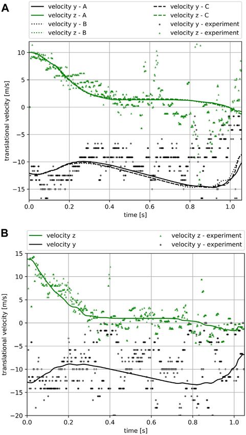
Sautter et al. Advanced Simulation of Attenuator Barriers
FIGURE 2 | (A) DEM-DEM rheological model adapted from Santasusana (2016). (B) DEM-FEM rheological model adapted from Santasusana (2016).
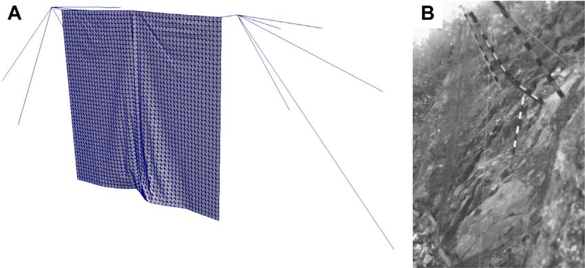
large deformations is the “loose” connection of the net to upper
ropes as illustrated in Figure 3. The net is connected orthogonal
to the dark blue support rope but is allowed to slide along the
rope, impeded only by friction.
To properly model this behavior in a FEM simulation a
sliding cable element formulation [Volkwein (2004), Boulaud
and Douthe (2017)] is employed, which also enables to
integrate a deflection roller into the simulation (left side of
Figure 3A).
Instead of single linear cable elements connecting the nodes ni
and ni+1 (see Figure 3B) the element formulation used in this
FIGURE 3 | Upper support rope. (A) Installation taken from Geobrugg
work considers all discrete nodes along a predefined path in one
(2019). (B) Sliding cable element, FEM discretization. single element. This is realized by computing the total strain of
the whole cable element with respect to the total length l instead
of the single lengths li . According to Volkwein (2004), Boulaud
the degrees of freedom u (here the displacements) and their second and Douthe (2017) the total length l in the current configuration
time derivative u€ zztu2 are integrated over the reference area Ω0 .
2
and the total length L in the reference configuration are calculated
This equilibrium is solved numerically with a Newton’s type as the sum of the respective line segments,
iterative solution technique operating on linearized virtual work nlines nlines
components as discussed in Belytschko et al. (2000). Internal l li , L Li . (4)
element forces Fint,r are expressed with respect to each degree of i i
freedom r in the system, according to,
As described in Belytschko et al. (2000), Holzapfel (2010) these
δW quantities are used to express the 1-dimensional Green-Lagrange
Fint,r . (2)
δur strain ε, and the 1-dimensional 2nd Piola-Kirchhoff stress S,
Additionally, the tangent stiffness matrix K, 1 l 2 − L2
ε , S E · ε, (5)
2 L2
zFint,r
Krs , (3)
zus with the help of the Young’s Modulus E. Including the prestress Spre
the virtual internal work δWint as stated in subsection 2.2 is expressed,
is often needed for Newton’s type solution schemes [see also
Belytschko et al. (2000), Holzapfel (2010)]. δWint Spre + S · δε dΩ0 ,
In the subsequent sections lower case symbols represent Ω0 (6)
quantities in the current configuration (x) while capital letters Spre + E · ε · A · L · δε,
describe quantities in the reference configuration (X).
In view of complex protective structures, such as Attenuator where A represents the reference cross-section of the cable
barriers, the structure must be modeled accurately with attention element. Following the derivation in Boulaud and Douthe
to detail. This work introduces the application of two unique (2017) an explicit formulation for δWint is developed,
finite element formulations to be used in the simulation of such
l
structures: the sliding cable element and the plane-stress δWint · A · E · ε + Spre · T · δu. (7)
membrane element. L
Equation 7 describes the virtual internal work of the sliding cable
2.2.1 Sliding Cable Element element with the help of the ratio between the total current length
Compliant structures, such as Attenuator barriers rely on the l and the total reference length L, including the vector of nodal
ability of large deformations to reduce peak decelerations and virtual displacements δu and the direction of internal forces at
withstand impacting objects. One feature which is used to realize each discrete node of the element assembled in vector T,
Frontiers in Built Environment | www.frontiersin.org 5 June 2021 | Volume 7 | Article 659382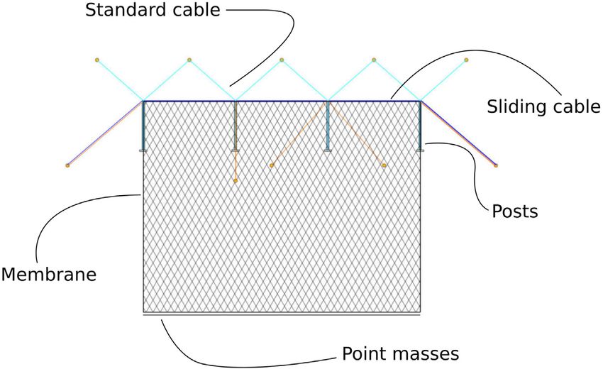
Sautter et al. Advanced Simulation of Attenuator Barriers
FIGURE 4 | Sliding cable elements on two opposing sides applying the tension field theory, described by Nakashino and Natori (2005), to exclude compression
stiffness from the plate in membrane finite elements. (A) Reference configuration, fixed on four corner nodes. (B) Sliding cable element formulation allows for a sliding of
the discrete element nodes.
Δx1 Δy1 Δz1 the general covariant base-vectors that span an arbitrary
T1 − − − , angled local coordinate system {Gi } and {gi } expressed by,
l1 l1 l1
Δxi−1 Δxi Δyi−1 Δyi Δzi−1 Δzi zNj j
Ti − − − , (8) Gi ·X, 2D : θ1 , θ 2 ,
li−1 li li−1 li li−1 li zθi
(9)
Δxn−1 Δyn−1 Δzn−1 zNj j
Tn . gi ·x, 2D : θ1 , θ 2 ,
ln−1 ln−1 ln−1 zθi
in which the standard FEM shape functions Ni are employed
Here n denotes the total number of nodes and the coordinates
(Belytschko et al., 2000). As the element is always a 2-dimensional
x, y, z describe the current configuration and the nodal coordinate
plane within a 3-dimensional frame, the base-vectors G3 and g3
distances, e.g., Δxi xi+1 − xi .
are constructed as a unit vector normal to that plane.
Additionally, the friction is included and needs to be evaluated
Belytschko et al. (2000) notes that these arbitrary base-vectors
at each discrete node in the element by first calculating an equal
are not necessarily orthonormal and are used to calculate the
and opposite force F i Fint,i and subsequently using this force
Green-Lagrange strain tensor ε,
to calculate a friction force ΔNi μF i according to the friction
coefficient μ. Volkwein (2004) discusses that this force must now 1
ε εij Gi ⊗ Gj gij − Gij Gi ⊗ Gj , (10)
be considered in addition to the normal elastic forces in the rope. 2
To validate the correct implementation of the sliding cable
where Gij and gij is the metric of the respective configuration and
element, a simple gravity driven impact simulation is illustrated
Gi expresses the reference contra-variant base-vectors.
in Figures 4A,B, demonstrating the expected large sliding
In order to express the elastic stress-strain relation S C : ε in
deformation of the net shackles.
clear matrix notation the stress and strain are arranged in Voigt
Alternative solutions to enable the sliding of nodes along a ~ · {~ε}. C describes a 4th order material
notation {•} yielding {~S} C
cable element can be achieved using the penalty method [see ~
tensor, while C is of 2 order.
nd
Bauer et al. (2018)], Lagrange multipliers [see Holzapfel
The anisotropic elastic consistent linearized tangent modulus
(2010)], or multi point constraints (MPC) as described in ~ from Münsch and Reinhardt (1995) dependent upon the
C
Abel and Shephard (1979). While the first two methods
Young’s Moduli Ex Ey , Poisson’s ratios ]xy , ]yx , and the shear
minimize the orthogonal distance between an arbitrary node
modulus G is expressed as,
and the axis of the sliding cable, the MPC approach directly
couples degrees of freedom in such a way that the node travels Ex ]xy Ex 0
~ 1 ⎢
⎡
⎢
⎢ ⎤⎥⎥⎥
along the desired path. Compared to these abstracted C ⎣ ]yx Ey
⎢ Ey 0 ⎥⎦, (11)
approaches, the sliding cable formulation, which inherently 1 − ]xy ]yx 0 0 1 − ]xy ]yx G
represents sliding nodes in its formulation, is the most robust ]xy ]yx
solution to the problem presented and adopted in this work. . (12)
Ey Ex
2.2.2 Plate in Membrane Action Since the {Gi } basis is not necessarily orthonormal, the strains
As described in Sasiharan et al. (2006), Dhakhal et al. (2011), naturally defined in that basis must be transformed to a local
Sautter et al. (2021) membrane finite elements are suitable to orthonormal basis {Ai } {Ai }. The construction of such a basis is
approximate the behavior and response of rock-fall cable nets. achieved by normalizing G1 and G3 creating A2 such that it is
With respect to the mesh geometry illustrated in Figure 6C, an orthonormal to A1 and A3 ,
anisotropic material law defined in Eq. 11 appropriately describes
G1 G3
the net’s direction-dependent behavior and is employed A1 , A3 ,
henceforth. |G1 | |G3 |
(13)
Derivation of the 2-dimensional plane-stress membrane G2 − G2 · A 1 A 1
A2 .
element within 3-dimensional space commences by defining |G2 − G2 · A1 A1 |
Frontiers in Built Environment | www.frontiersin.org 6 June 2021 | Volume 7 | Article 659382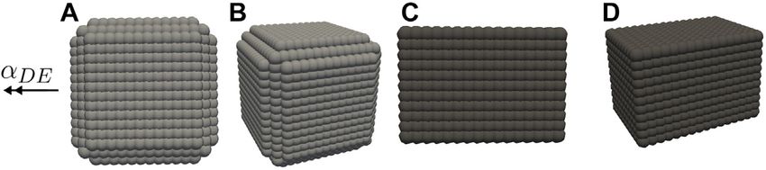
Sautter et al.                                                                                                              Advanced Simulation of Attenuator Barriers

  FIGURE 5 | Strong coupling communication diagram from Sautter et al. (2020). With t as the current time and Δt as the time step size.

The covariant strain coefficients ~εij in the local orthonormal basis                         convergent strong coupling as described by Sautter et al. (2020)
{Ai } transform by the following rule, given in Kiendl (2011),                               (which also includes more details of the coupling).
                                                                                                The steps in Figure 5 are summarized below:
                       ~εkm  εij · Ak · Gi  · Gj · Am .                      (14)
                                                                                                  1. Solve DEM component to obtain the contact force.
2.3 Coupling Procedure                                                                            2. Map the forces to the structure.
A partitioned coupling approach is employed to couple                                             3. Solve the structure with FEM to obtain nodal
independent discrete element and finite element methods                                               displacements, velocities and accelerations.
together in this work. Felippa et al. (2001) note that                                            4. Map displacements, velocities and accelerations back to
partitioned solution schemes possess the notable benefits of                                          the discretized boundary in the DEM solver.
software modularity and also application of the most                                              5. If necessary: Calculate interface residuals as described by
appropriate discretization and solution techniques to each                                           Küttler and Wall (2008), Winterstein et al. (2018), Sautter
individual component. Although this approach allows the use                                          et al. (2020) among others.
of arbitrary DEM and FEM codes, the user must consider the                                        6. If necessary: Repeat steps 1–5 until Eqs 15–17 are satisfied
coupling of the two. Santasusana (2016) has already discussed this                                   to a given tolerance.
in detail and Sautter et al. (2020) has continued this coupling by                                7. Advance in time to next time step.
introducing an additional Gauss-Seidel loop on the interface Γ
level to ensure the convergence of the interface. The basic idea of
the coupling method is the exchange of data between the two                                  3 2017 GEOBRUGG ROCKFALL
independent solvers. The solver of the DEM calculates contact
                                                                                             EXPERIMENTS
forces Fcontact which are dependent on the displacements u and
velocities u_ of the particles P and the discretized boundary                                In 2017 the Swiss company Geobrugg conducted an experimental
conditions ΩD . These forces are mapped [see e.g., Tianyang                                  program to confirm the effectiveness of a novel SPIDER mesh
(2016)] to the finite element mesh of the structure ΩS and by                                 (Geobrugg, 2020). The following section is a brief summary of key
means of FEM the displacements and velocities are calculated                                 test aspects relevant for numerical replication, refer to Hofmann
which are finally mapped to the boundary conditions of the DEM                                et al. (2019) for full testing details.
solver. Multiple studies Wüchner (2006), Winterstein et al.
(2018), Sautter et al. (2020) have confirmed that the simple                                  3.1 Test Site
exchange of this data can lead to divergence of the interface                                The test site was a near-vertical approximately 60 m high slope
conditions,                                                                                  situated in a disused granite quarry in British Columbia, Canada.
                                                                                             The Attenuator design investigated was the hanging net style with
                               uΩD,Γ (t) − uΩS,Γ (t)  0,                         (15)       limited slope contact of the netting as per Figure 6A. The test set
                                ΩD,Γ                ΩS,Γ
                               u_      (t) − u_            (t)  0,               (16)       up consisted of three 8 m steel posts set 9 m apart and anchored to
                           ΩD,Γ              ΩD,Γ                                            the slope with six retention ropes, two lateral support ropes, and
                 Fcontact u        (t), u_         (t), u (t), u_ (t)
                                                             P        P
                                                                                             one top rope penetrating through the post heads. The netting is
                    − Fcontact u    ΩS,Γ
                                            (t), u_ ΩS,Γ (t), uP (t), u_ P (t)              attached to the top rope with shackles in each mesh opening as
                     0,                                                          (17)       detailed in Figure 3A. Three principal zones of attenuation were
                                                                                             investigated by varying the impact, transition, and collection
all of which are dependent on the time t. Figure 5 describes the                             zones of the high tensile steel wire nets. The experiments of
use of additional iteration loops at each time step to achieve the                           2017 are described in greater detail in Hofmann et al. (2019).

Frontiers in Built Environment | www.frontiersin.org                                     7                                      June 2021 | Volume 7 | Article 659382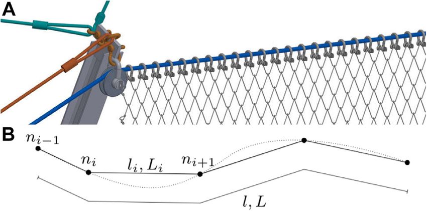
Sautter et al.                                                                                                             Advanced Simulation of Attenuator Barriers

  FIGURE 6 | Experiment setup. (A) Additional weight at the bottom of the protection net to ensure a more controlled structural deformation. (B) Photo of the
                                                                                                                                                          ®
  impacting object T092 (some damage can be observed). The visible metal cap covers the housing of the motion sensors. (C) Technical drawing of the SPIDER S4-130,
  taken from Geobrugg (2020), DL  8.6 mm.

3.2 Site Survey and Rockfall Modeling                                                 every 90+ rotation of the block served as an indicative
A terrain survey of the site was performed by Truline Survey in                       quantification of angular velocity. The cameras were
2016 which was used as basis for rockfall modeling to adapt the                       located so as to have a frontal view on the mesh and a
Attenuator geometry between the testing series of 2016 and 2017.                      perpendicular view on the mesh. This allowed also to
Particularly relevant to this paper, Sautter et al. (2020)                            determine in which plane the block was moving.
demonstrates how such terrain models may be incorporated
into simulations to further enhance accuracy and predictive                           3.4.2 Rock Motion Sensors
confidence.                                                                            The rock motion sensors measured the accelerations and
                                                                                      rotations of the block about its three axes for the duration of
3.3 Impacting Object                                                                  each test. A comparison of the angular velocity obtained from the
The rocks used for testing were either granite blocks of various                      video analysis and the rock motion sensor shows good agreement
characteristic shapes (such as cubic, angular, and disc-like) or                      and therefore provides confidence in the translational velocity
prefabricated concrete blocks with a special housing in the center                    data estimated by video analysis.
for rock motion sensors (see Figure 6B). The blocks and rocks
were then released by an excavator on top of the slope. The rocks                     3.5 Tests Used for Numerical Validation
bounced 3–4 times on the granite slope before impacting the                           The tests used to validate the modeling and simulation used a
netting.                                                                              Geobrugg SPIDER S4/130 mesh [described in Geobrugg (2020)
                                                                                      and visualized in Figure 6C]. Additional weights in the form of
3.4 Instrumentation                                                                   steel bars were shackled to the bottom of the mesh (see Figure 6A)
Experimental instrumentation included load-cells in all ropes,                        to increase the inertia and vertically pre-tension the system and is
high-speed cameras filming the block’s trajectory from different                       incorporated in the simulation with additional point masses
angles and rock motion sensors in the concrete blocks. This work                      (discussed in subsection 4.1.1). The middle post was slightly
will predominantly focus on the trajectory path, translational                        bent after sustaining two rock impacts in previous tests, but the
velocity and rotational velocity experimental data collected.                         integrity and function of the system was not compromised,
                                                                                      accordingly testing was continued, but it was chosen to
3.4.1 High Speed Cameras                                                              incorporate it anyway in the modeling of the structure. The
Analysis of the high speed camera videos with a sampling rate                         blocks used during the test, were a near-cubic 626 kg concrete
of 500 fps facilitated quantification of the rockfall dynamics.                        block with an initial volume of approximately 0.75 × 0.75 ×
By tracking the position of the block through time a                                  0.75m3 called T092 and a 278kg granite block with an initial
translational velocity could be obtained and the tracking of                          volume of approximately 0.75 × 0.51 × 0.48m3 called T089. Since

Frontiers in Built Environment | www.frontiersin.org                              8                                            June 2021 | Volume 7 | Article 659382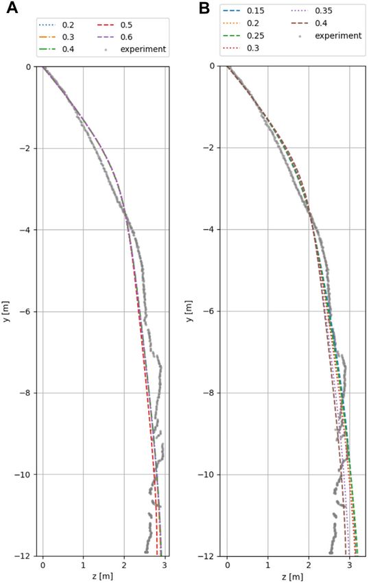
Sautter et al.                                                                                                 Advanced Simulation of Attenuator Barriers

  FIGURE 7 | Participants in the FEM model, adapted from Geobrugg (2019).

the blocks were used for several tests and accumulated greater                  discussed in subsection 2.2.1. This formulation allows
damage after each run (see Figure 6B for T092), the mass before                 internal nodes to slide along the element, while internal
and after each run was the characterizing measurement (instead                  forces are calculated based on the change of the total
of volume).                                                                     length, as discussed in Volkwein (2004); Boulaud and
   Key experimental data pertinent to numerical replication                     Douthe (2017). The following structural properties, based
including translational and rotational velocity at the time of                  on construction plans in Geobrugg (2019), were applied in
netting impact and the rock’s path and mass are summarized                      the simulation: Young’s Modulus E  1.130 · 1011 [N/m2 ], cross
in subsection 4.2.                                                              area A  1.645 · 10− 4 [m2 ], density ρ  7.850 · 103 [kg/m3 ], and
                                                                                the friction coefficient μ  0.25.

4 NUMERICAL MODELING                                                            4.1.3 Standard Cable Element
                                                                                Bracing cables, modeled with standard cable elements, are
4.1 Structural Modeling                                                         anchored in the rock and connected to strategically selected
Figure 7 is adapted from Geobrugg (2019) and depicts the                        points on the supports of the protective structure. As presented
respective participants in the simulation, each of which are                    in Belytschko et al. (2000), a 1-dimensional truss element
discussed below.                                                                formulation is applied and combined with an additional
   Due to the small time steps necessary to resolve the impact, an              check for compression stresses in the element. If such
explicit time integration scheme was selected (instead of an                    stresses are detected the elemental stiffness contribution is
implicit scheme). The central-difference explicit scheme as                     temporarily eliminated from the global system of equations.
described by Belytschko et al. (2000) was used to conduct the                   Realistic structural properties were also obtained from
numerical time integration of the structural response with a time               construction plans provided in Geobrugg (2019) and listed
step of dt  5 · 10− 5 s.                                                       in the following: Young’s Modulus E  1.100 · 1011 [N/m2 ],
                                                                                cross area A  1.160 · 10− 4 [m2 ], and density ρ  7.850 ·
4.1.1 Point Masses                                                              103 [kg/m3 ].
The additional weights at the bottom of the protection net,
depicted in Figure 6, are modeled with single point masses                      4.1.4 Posts
(summing to an additional total mass of Madd  358kg)                           The posts, which predominantly carry vertical loads to support
equally distributed along the lower boundary of the membrane                    the protective structure, are simply supported in the rock. At the
mesh (see Figure 7). Including these masses is critical to properly             top they are connected to both the upper support rope as well as
model both the gravitational forces and the additional dynamic                  the bracing cables (seeFigure 3). In accordance with Belytschko
inertia.                                                                        et al. (2000), these posts may be suitably modeled as 1-
                                                                                dimensional truss elements (neglecting any initial damaged
4.1.2 Sliding Cable Element                                                     bending), with the following data: Young’s Modulus
Modeling of the upper support rope, illustrated in Figure 3,                    E  2.100 · 1011 [N/m2 ], cross area A  2.010 · 10− 3 [m2 ], and
demands a sophisticated element formulation, which is                           density ρ  7.850 · 103 [kg/m3 ].

Frontiers in Built Environment | www.frontiersin.org                        9                                      June 2021 | Volume 7 | Article 659382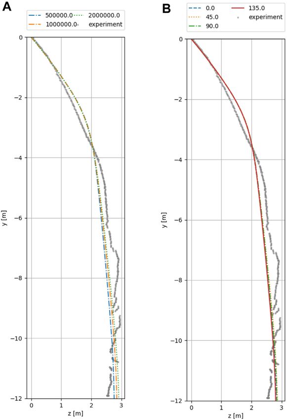
Sautter et al.                                                                                                            Advanced Simulation of Attenuator Barriers

  FIGURE 8 | Deformation panel after dead-load equilibrium (before impact). (A) Simulation. (B) Experiment photographed just before impact.

4.1.5 Protection Net                                                                  Santasusana et al. (2016). Figure 9 presents the DEM cluster
Due to the set-up of the experiment, similar to the set-up in                         models used within this work, and Figure 6B shows the real
Sautter et al. (2021), and the complicated geometry of the SPIDER                     impacting object. While the clusters in Figures 9A,B represent
net system (see Figure 6C), the net has been idealized as a closed                    the test object T092, Figures 9C,D show the cluster
homogeneous surface discretized with plane-stress membrane                            approximation of the test object T089. A study on the proper
finite elements. Publications such as Mentani et al. (2018),                           refinement level of such clusters can be found in Sautter et al.
Tahmasbi et al. (2019) suggest shell elements to be used,                             (2021). Special algorithms are required to create the refined cluster
although they introduce additional complexity and                                     file, with this work employing the algorithms described in Bradshaw
computational expense compared to membrane elements. In                               and O’Sullivan (2002), Bradshaw and O’Sullivan (2004) available in
the interest of simplicity, membrane elements described in                            an online toolkit [http://isg.cs.tcd.ie/spheretree/].
subsection 2.2.2 were employed, which, considering the good                               Within this work several DEM particle properties are varied
agreement achieved with experimental results in section 5,                            and their influence on the simulation result is studied, namely the
appear sufficiently accurate for the present study.                                    friction, coefficient of restitution, and Young’s Modulus.
   The following properties, determined from the mesh technical                       Contrasting this, the following physical properties are constant
drawing in Figure 6C, technical data sheets (Geobrugg, 2020) and                      throughout all simulation runs:
proprietary Geobrugg experimental tensile tests, were applied to
membrane elements for the simulation: Thickness                                       - T092
8.600 · 10− 3 [m], Young’s Modulus Ex  0.23 · 108 [N/m2 ],                              - Mass  6.26 · 102 [kg],
Young’s          Modulus         Ey  1.40 · 108 [N/m2 ],    shear                       - Dimension ≈ 0.75 × 0.75 × 0.75[m3 ],
modulus G  0.81 · 10 [N/m ], Poisson’s ratio ]xy  0.30, and
                         8      2                                                        - Impact translational velocity horizontal u_ z  10.01[m/s],
density ρ  5.814 · 102 [kg/m3 ].                                                        - Impact      translational    velocity    vertical     (gravity
   Although the material behavior is in principle non-linear, the                          direction) u_ y  −12.08[m/s],
large deformations are predominantly rigid and accompanied by                            - Impact rotational velocity ω  22.0[rad/s].
small strains, justifying the assumption of linear elastic material                   - T089
behavior.                                                                                - Mass  2.78 · 102 [kg],
   By comparing Figures 8A,B a perfect agreement between                                 - Dimension ≈ 0.75 × 0.51 × 0.48[m3 ],
the reference computer model and the real structure cannot                               - Impact translational velocity horizontal u_ z  13.78[m/s],
be achieved as some posts in Figure 8B are already                                       - Impact      translational    velocity    vertical     (gravity
damaged. Additionally, the position and alignment of the                                   direction) u_ y  −12.78[m/s],
supporting structure is unlikely to exactly match                                        - Impact rotational velocity ω  10.0[rad/s].
construction plans.
                                                                                         Comparing Figures 6B, 9A it can be observed that the testing
4.2 Impacting Object                                                                  objects have already suffered damage from previous experiments.
In contrast to preceding works, such as Volkwein (2004),                              When comparing the simulation results with the ones obtained
Volkwein (2005), Mentani et al. (2018) this work follows                              by the experiment in section 5 this unavoidable difference should
Sautter et al. (2021) to flexibly model arbitrary objects with                         be considered.
discrete spherical element clusters. The advantage compared to                           An explicit central-difference scheme as described by Matuttis
standard finite element discretized objects is the simplified                           and Chen (2014) was used to conduct the numerical time
contact detection between arbitrary boundary objects and                              integration of the translational velocity of the cluster with a
single spheres contained in the cluster as described by                               time step of dt  5 · 10− 5 s. As presented in Irazábal et al.

Frontiers in Built Environment | www.frontiersin.org                             10                                           June 2021 | Volume 7 | Article 659382
Sautter et al. Advanced Simulation of Attenuator Barriers
FIGURE 9 | Cluster of spheres to model impacting objects. (A) Test object T092 front view. (B) Test object T092 perspective view. (C) Test object T089 front view.
(D) Test object T089 perspective view.
(2019), a more sophisticated time integration approach was used
to integrate the rotational velocity using quaternions (Hamilton.
1844), which is especially critical due to the non-uniform
geometry of the impacting clusters as shown in Figure 9.
5 VALIDATION
The following section presents the simulated Geobrugg 2017
experiment results to ascertain the practical applicability and
accuracy of the aforementioned numerical modeling approaches
and technologies.
For clarity, key assumptions and uncertainties discussed in the
preceding sections are summarized below:
- The exact impact location was estimated from video
records.
- The model of the protective structure is taken from
construction plans. However, it can be seen from
photos and video recordings that the actual structure is
partially crooked and already shows damage.
- The reference angular orientation αDE of the impacting
object describes the rotation around the main axis of the
impacting object at the time of impact. It cannot be
determined and is therefore included in the following
investigation as an unknown variable. This also means
that the angular velocities cannot be absolutely
compared. The orientation of αDE is visualized in
Figure 9A.
- Three further DEM specific parameters cannot be taken
unambiguously from the test and have to be varied to
study their influence. Young’s Modulus EDE , coefficient of
restitution ϵDE and friction μDE are partly problem-
FIGURE 10 | Visualization of object path for varying parameters for
dependent and their influence is not well researched T092. (A) Coefficient of restitution. The result data for 0.2, 0.3, 0.4, and 0.6 are
with regard to Attenuator barriers. nearly identical and thus hardly distinguishable in the graph. (B) Friction.
- As visualized in Figure 6B the impacting test object
already shows damage, which will be neglected in the
modeling of the DEM sphere cluster. barriers are used to protect exposed areas such as motorways
from falling rocks, therefore the path of the object is of particular
The rock trajectory and the general trends of angular and interest. In the following investigation the unknown model
translational velocities are used for comparison with the experiment. parameters were varied to check their influence on the results
of the test run T092. To validate the results the test T089 was
5.1 Trajectories simulated subsequently with the best suitable parameters
The most reliable and functionally-important comparison is the obtained from the investigation of T092. Figures 10, 11
simulated versus experimental rock trajectory. Attenuator illustrate the influence of the DEM parameters for T092
Frontiers in Built Environment | www.frontiersin.org 11 June 2021 | Volume 7 | Article 659382Sautter et al. Advanced Simulation of Attenuator Barriers
FIGURE 11 | Visualization of object path for varying parameters for
T092. (A) Young’s Modulus [N/m2 ]. (B) Angular reference orientation [+ ].
FIGURE 12 | Visualization of object path. Additionally, the free fall
trajectory is added to demonstrate the correctness of the object path at the
(which are not clearly defined and have to varied to study their beginning of the simulation and the effectiveness of the Attenuator barrier. (A)
The three optimal parameter combinations for T092. The solution for
influence). parameter set B is very similar to the one for parameter set A and thus not
easily distinguishable. (B) T089 with parameter set C.
- In Figure 10A the coefficient of restitution is varied
between 0.2 − 0.6 while the Young’s Modulus
EDE 2000000N/m2 , the friction μDE 0.4, and the (see subsection 2.1). The range of EDE in this work does not represent
reference angular orientation αDE 146.25+ . the physical properties of concrete but proved to result in the best
- In Figure 10B the friction is varied between 0.15 − 0.4 fitting results. This could also be observed when the obtained
while the Young’s Modulus EDE 2000000N/m2 , the parameters were used to simulate the test run T089 (see
coefficient of restitution ϵDE 0.6, and the reference Figure 12B). Figure 11A demonstrates that EDE does not heavily
angular orientation αDE 146.25+ . influence this kind of simulation and further studies showed that
- In Figure 11A the Young’s Modulus is varied between choosing a EDE to be near the physical value of the Young’s Modulus
500000N/m2 − 2000000N/m2 while the coefficient of of concrete does not influence the simulation result but will lead to the
restitution ϵDE 0.6, the friction μDE 0.4, and the necessity of much smaller times steps, contradicting the purpose of
reference angular orientation αDE 146.25+ . this work to offer a fast, efficient, simplified model and simulation of
- In Figure 11B the reference angular orientation is varied the Attenuator barriers.
between 0+ − 135+ while the Young’s Modulus An initial observation is that all variations give very good
EDE 2000000N/m2 , the coefficient of restitution agreement with the test results for T092 and accurately predict
ϵDE 0.6, the friction μDE 0.4. the final position of the rock with a maximum error of +10%.
While varying the reference angular orientation seems to have the
While the deformation of the impacting object is not of interest for least influence (see Figure 11B) the proper choice of a suitable
this study the so-called Young’s Modulus EDE represents only an friction value strongly influences the simulation as shown in
algorithmic parameter in the calculation of the DEM contact forces Figure 10B. This sensitivity is expected as this experiment heavily
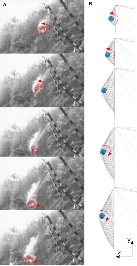
Frontiers in Built Environment | www.frontiersin.org 12 June 2021 | Volume 7 | Article 659382Sautter et al. Advanced Simulation of Attenuator Barriers FIGURE 13 | The test object impacts with a certain angular velocity, stops rotating, slides for a short time period and starts rotating in the opposite direction subsequently. (A) Photos from the experiment. (B) Simulation. Frontiers in Built Environment | www.frontiersin.org 13 June 2021 | Volume 7 | Article 659382
Sautter et al.                                                                                                              Advanced Simulation of Attenuator Barriers

  FIGURE 14 | Visualization of angular velocity about one of the main axis of the impacting object T092. (A) Simulation. (B) General trend from experiment.

depends on the rotation of the impacting object. The variation of                                                  gravity

the Young’s Modulus in Figure 11A as well as the variation of the                                       m     1          m
                                                                                          12.00m  12.08 · t + · 9.81 2 · t 2                 →        t  0.76s,
coefficient of restitution in Figure 10A show little influence, likely                                    s     2          s
since the Attenuator barrier primarily retards via kinetic energy                                                                                               (18)
instead of strain energy.
                                                                                          0.76s to reach the ground. In combination with an initial
    In the following, only the three best parameter variants for T092
                                                                                       horizontal velocity of 10.01m/s the stone will have traveled a
will be discussed, as the quality of the trajectories allows direct
                                                                                       horizontal distance of 10.01 ms · 0.76s ≈ 7.6m. This results in a
conclusions to be drawn about the correctness of the respective
                                                                                       potential risk area that is approximately three times as large as for
velocities. The three optimal parameter combinations are presented
                                                                                       the protective installation (compare Figure 12A).
in the following list and their trajectories are visualized in Figure 12A
                                                                                          The results, which are shown in Figure 12B relate to the
together with the path of a free falling object to demonstrate the
                                                                                       simulation of T089 with the parameter set C of T092. It can be
efficacy of the Attenuator barrier.
                                                                                       clearly seen that the experimental results are properly re-
                                                                                       produced without any further need of parameter investigation.
- Parameter set A:
                                                                                       This ensures that this parameter set can be used to recalculate
   - Friction μDE  0.4,
                                                                                       further scenarios and creates confidence in the accuracy and
   - Coefficient of restitution ϵDE  0.6,
                                                                                       applicability of the study presented here.
   - Young’s Modulus EDE  1 · 106 [N/m2 ],
   - Reference angular orientation αDE  146.25[+ ].
- Parameter set B:                                                                     5.2 Angular Velocity
   - Friction μDE  0.4,                                                               The experimental observations presented in Figure 13A illustrate
   - Coefficient of restitution ϵDE  0.6,                                              the impacting object angularly decelerating and subsequently
   - Young’s Modulus EDE  2 · 106 [N/m2 ],                                            accelerating in the opposing angular direction. Unfortunately,
   - Reference angular orientation αDE  168.75[+ ].                                   the experimental data do not provide any information about
- Parameter set C:                                                                     predominate rotation axis, the individual rotation components of
   - Friction μDE  0.4,                                                               each axis, or the rotational orientation of the specimen at the time
   - Coefficient of restitution ϵDE  0.3,                                              of impact. Nevertheless, it is useful to compare the general
   - Young’s Modulus EDE  2 · 106 [N/m2 ],                                            rotation behavior with the simulation results, with Figure 13B
   - Reference angular orientation αDE  45[+ ].                                       illustrating the simulation exhibits the same rotational trend as
                                                                                       the experiment in Figure 13A. Additionally, Figure 14A
   The data obtained from the simulations is not only in strong                        visualizes the angular velocity about one of the main axes of
accordance with the experiment results but also clearly                                the impacting object, which clearly illustrates the time period in
demonstrates the effectiveness of the herein presented                                 which the aforementioned deceleration and subsequent
Attenuator barrier. A rock at height of 12m with an initial                            acceleration take place. The same behavior can be observed in
vertical velocity in gravity direction of 12.08m/s (as it is the                       Figure 14B, which depicts the general trend of the angular
case for T092) would need,                                                             velocity obtained from the experiment.

Frontiers in Built Environment | www.frontiersin.org                              14                                            June 2021 | Volume 7 | Article 659382
Sautter et al. Advanced Simulation of Attenuator Barriers
statements to be made about future rockfall events in Attenuator
barriers.
6 CONCLUSION
This work has applied an advanced modeling and simulation
approach to characterize the behavior of Attenuator barriers.
Two independent numerical methods were coupled within an
open-source multi-physics code to analyze the interaction of the
impacting object and the protective structure. The impacting
objects were simulated using DEM whereby arbitrarily shaped
rocks were flexibly modeled as clusters of single spherical particles.
This effective procedure allows the simultaneous use of simple
contact algorithms and the possibility to consider the influence of
arbitrary rock shapes. The structure itself was simulated using FEM
employing a variety of advanced element formulations appropriate
for each structural component. A homogeneous anisotropic
membrane element was used to simplify the complicated
protection mesh. As in Sautter et al. (2021), this simplification
was found to be applicable when the global deformation behavior
has to be investigated. A sophisticated yet elegant sliding cable
formulation was applied to model the sliding nodes on the support
ropes, allowing the boundary kinematics of the net to be fully
resolved. Due to the robust implementation in the open-source
code KRATOS [see Dadvand et al. (2010), Dadvand et al. (2013);
Ferrándiz et al. (2020)], this work allows engineers and researchers
alike to perform independent analyses of any rockfall event and the
evaluation of suitable protection structures.
Another objective of this work was evaluating the performance
of Attenuator barriers. It was demonstrated that this type of flexible
protective structure offers dramatically increased protection
against rockfalls by retarding impacts and subsequently guiding
them to designated collection zones. In subsection 5.1 the
simulation and experimental results agree that the Attenuator
barrier considered reduced the danger zone by approximately
FIGURE 15 | Comparison of translational velocity for both the horizontal two thirds compared to a free falling object. The fact that the
direction, z and the vertical in gravity direction, y. (A) The three optimal Young’s modulus and the coefficient of restitution of the DEM
parameter combinations for T092. (B) T089 with parameter set C. cluster have little influence on the trajectory of the impacting object
was expected, since little energy is absorbed by strains and internal
forces and the rock is instead deflected. On the other hand, the
5.3 Translational Velocity correct choice of interface friction was found to be important, as
The translational velocity of the three optimal parameter sets (as the experimental data is strongly influenced by the rotation of the
per subsection 5.1) and the experiment are illustrated in impacting object. To support the conclusions of this study, another
Figure 15A. It can be seen that the deceleration of the test was simulated without varying the unknown parameters. The
impacting rock in the horizontal direction (perpendicular to set of best parameters from the previous tests was applied directly.
the protection net) is accurately modeled by the simulation. The results of this work clearly show that with this procedure the
This is of particular importance for the design of protection experimental results can be calculated with a very good agreement.
structures, since the management of horizontal momentum is the Thus, future questions regarding Attenuator barriers can be
primary arresting mechanism. Although experimental results for answered confidently, quickly and efficiently. The CPU system
the vertical (gravity) direction are substantially scattered, the settings for this study is an Intel(R) Xeon(R) CPU E5-2,623 v4 at
simulation demonstrates a good agreement with the general 2.60GHz, while it takes approximately 700 s (11.667 min) to run
trend of the experimental data. one simulation.
Just as in subsection 5.1, the velocity components of the Live experiments are time-consuming and very costly,
simulation and the experiment of T089 are also compared in the especially if every new change in the design has to be
following. Figure 15B shows that these data could also be investigated experimentally. The numerical analysis of these
reproduced with very good agreement and thus allows suitable tests can support the design process and thus make the
Frontiers in Built Environment | www.frontiersin.org 15 June 2021 | Volume 7 | Article 659382You can also read