Neural Predictive Monitoring under Partial Observability
←
→
Page content transcription
If your browser does not render page correctly, please read the page content below
Neural Predictive Monitoring
                                                               under Partial Observability

                                                        Francesca Cairoli1, Luca Bortolussi1,2, and Nicola Paoletti3
                                                1
                                                     Department of Mathematics and Geosciences, Università di Trieste, Italy
                                                       2
                                                         Modeling and Simulation Group, Saarland University, Germany
arXiv:2108.07134v2 [cs.LG] 17 Aug 2021

                                                    3
                                                      Department of Computer Science, Royal Holloway University, London

                                                Abstract. We consider the problem of predictive monitoring (PM), i.e., pre-
                                                dicting at runtime future violations of a system from the current state. We
                                                work under the most realistic settings where only partial and noisy observations
                                                of the state are available at runtime. Such settings directly affect the accuracy
                                                and reliability of the reachability predictions, jeopardizing the safety of the
                                                system. In this work, we present a learning-based method for PM that produces
                                                accurate and reliable reachability predictions despite partial observability (PO).
                                                We build on Neural Predictive Monitoring (NPM), a PM method that uses deep
                                                neural networks for approximating hybrid systems reachability, and extend it to
                                                the PO case. We propose and compare two solutions, an end-to-end approach,
                                                which directly operates on the rough observations, and a two-step approach,
                                                which introduces an intermediate state estimation step. Both solutions rely
                                                on conformal prediction to provide 1) probabilistic guarantees in the form of
                                                prediction regions and 2) sound estimates of predictive uncertainty. We use the
                                                latter to identify unreliable (and likely erroneous) predictions and to retrain
                                                and improve the monitors on these uncertain inputs (i.e., active learning). Our
                                                method results in highly accurate reachability predictions and error detection,
                                                as well as tight prediction regions with guaranteed coverage.

                                         1    Introduction
                                         We focus on predictive monitoring (PM) of cyber-physical systems (CPSs), that is, the
                                         problem of predicting, at runtime, if a safety violation is imminent from the current
                                         CPS state. In particular, we work under the (common) setting where the true CPS
                                         state is unknown and we only can access partial (and noisy) observations of the system.
                                            With CPSs having become ubiquitous in safety-critical domains, from autonomous
                                         vehicles to medical devices [4], runtime safety assurance of these systems is paramount.
                                         In this context, PM has the advantage, compared to traditional monitoring [6], of
                                         detecting potential safety violations before they occur, in this way enabling preemptive
                                         countermeasures to steer the system back to safety (e.g., switching to a failsafe mode as
                                         done in the Simplex architecture [18]). Thus, effective PM must balance between predic-
                                         tion accuracy, to avoid errors that can jeopardize safety, and computational efficiency,
                                         to support fast execution at runtime. Partial observability (PO) makes the problem
                                         more challenging, as it requires some form of state estimation (SE) to reconstruct the
                                         CPS state from observations: on top of its computational overhead, SE introduces
                                         estimation errors that propagate in the reachability predictions, affecting the PM
                                         reliability. Existing PM approaches either assume full state observability [9] or cannot
                                         provide correctness guarantees on the combined estimation-prediction process [13].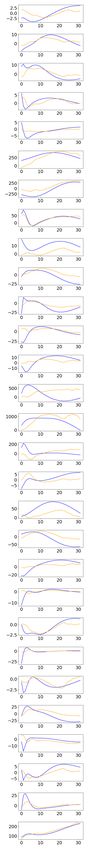
2       F. Cairoli et al.

   We present a learning-based method for predictive monitoring designed to produce
efficient and highly reliable reachability predictions under noise and partial observability.
We build on neural predictive monitoring (NPM) [9,10], an approach that employs
neural network classifiers to predict reachability at any given state. Such an approach is
both accurate, owing to the expressiveness of neural networks (which can approximate
well hybrid systems reachability given sufficient training data [26]), and efficient, since
the analysis at runtime boils down to a simple forward pass of the neural network.
   We extend and generalize NPM to the PO setting by investigating two solution
strategies: an end-to-end approach where the neural monitor directly operates on the
raw observations (i.e., without reconstructing the state); and a two-step approach,
where it operates on state sequences estimated from observations using a dedicated
neural network model. See Fig 1 for an overview of the approach.
   Independently of the strategy chosen for handling PO, our approach offers two ways of
quantifying and enhancing PM reliability. Both are based on conformal prediction [5,34],
a popular framework for reliable machine learning. First, we complement the predictions
of the neural monitor and state estimator with prediction regions guaranteed to cover
the true (unknown) value with arbitrary probability. To our knowledge, we are the
first to provide probabilistic guarantees on state estimation and reachability under PO.
Second, as in NPM, we use measures of predictive uncertainty to derive optimal criteria
for detecting (and rejecting) potentially erroneous predictions. These rejection criteria
also enable active learning, i.e., retraining and improving the monitor on such identified
uncertain predictions.
   We evaluate our method on a benchmark of six hybrid system models. Despite PO, we
obtain highly accurate reachability predictions (with accuracy above 99% for most case
studies). These results are further improved by our uncertainty-based rejection criteria,
which manage to preemptively identify the majority of prediction errors (with a detection
rate close to 100% for most models). In particular, we find that the two-step approach
tends to outperform the end-to-end one. The former indeed benefits from a neural SE
model, which provides high-quality state reconstructions and is empirically superior
to Kalman filters [35] and moving horizon estimation [2],two of the main SE methods.
Moreover, our method produces prediction regions that are efficient (i.e., tight) yet
satisfy the a priori guarantees. Finally, we show that active learning not just improves
reachability prediction and error detection, but also increases both coverage and efficiency
of the prediction regions, which implies stronger guarantees and less conservative regions.

Fig. 1. Overview of the NPM framework under partial observability. The components used at
runtime have a thicker border.
Neural Predictive Monitoring under Partial Observability            3

2      Problem Statement
We consider hybrid systems (HS) with discrete time and deterministic dynamics and
state space S =V ×Q, where V ⊆Rn is the domain of the continuous variables, and
Q is the set of discrete modes.
          vi+1 =Fqi (vi,ai,ti); qi+1 =Jqi (vi); ai =Cqi (vi); yi =µ(vi,qi)+wi,         (1)
    where vi =v(ti), qi =q(ti), ai =a(ti), yi =y(ti) and ti =t0 +i·∆t. Given a mode q ∈Q,
Fq is the mode-dependent dynamics of the continuous component, Jq is mode switches
(i.e., discrete jumps), Cq is the (given) control law. Partial and noisy observations
yi ∈Y are produced by the observation function µ and the additive measurement noise
wi ∼W (e.g., white Gaussian noise).
    Predictive monitoring of such a system corresponds to deriving a function that
approximates a given reachability specification Reach(U,s,Hf ): given a state s=(v,q)
and a set of unsafe states U, establish whether the HS admit a trajectory starting from
s that reaches U in a time Hf . The approximation is w.r.t. some given distribution
of HS states, meaning that we can admit inaccurate reachability predictions if the state
has zero probability. We now illustrate the PM problem under the ideal assumption
that the full HS can be accessed.
Problem 1 (PM for HS under full observability). Given an HS (1) with state space
S, a distribution S over S, a time bound Hf and set of unsafe states U ⊂ S, find a
function h∗ :S →{0,1} that minimizes
                                     the probability
                                 ∗

                        P rs∼S h (s)6= 1 Reach(U,s,Hf ) ,
where 1 is the indicator function. A state s ∈ S is called positive w.r.t a predictor
h:S →{0,1} if h(s)=1. Otherwise, s is called negative.
  As discussed in the next section, finding h∗, i.e., finding a function approximation
with minimal error probability, can be solved as a supervised classification problem,
provided that a reachability oracle is available for generating supervision data.
  The problem above relies on the assumption that full knowledge about the HS state is
available. However, in most practical applications, state information is partial and noisy.
Under PO, we only have access to a sequence of past observations yt =(yt−Hp ,...,yt)
which are generated as per (1), that is, by applying the observation function µ and
measurement noise to the unknown state sequence st−Hp ,...,st.
  In the following, we consider the distribution Y over Y Hp of the observations se-
quences yt =(yt−Hp ,...,yt) induced by state st−Hp ∼S, HS dynamics (1), and iid noise
wt =(wt−Hp ,...,wt)∼W Hp .
Problem 2 (PM for HS under noise and partial observability). Given the HS and
reachability specification of Problem
                                     1, find a function g∗ :Y Hp →{0,1} that minimizes
                                    ∗

                         P ryt ∼Y g yt =  6 1 Reach(U,st,Hf ) .
   In other words, g∗ should predict reachability values given in input only a sequence
of past observations, instead of the true HS state. In particular, we require a sequence
of observations for the sake of identifiability. Indeed, for general non linear systems,
a single observation does not contain enough information to infer the HS state4.
 4
     Feasibility of state reconstruction is affected by the time lag and the sequence length. Our
     focus is to derive the best predictions for fixed lag and sequence length, not to fine-tune
     these to improve identifiability.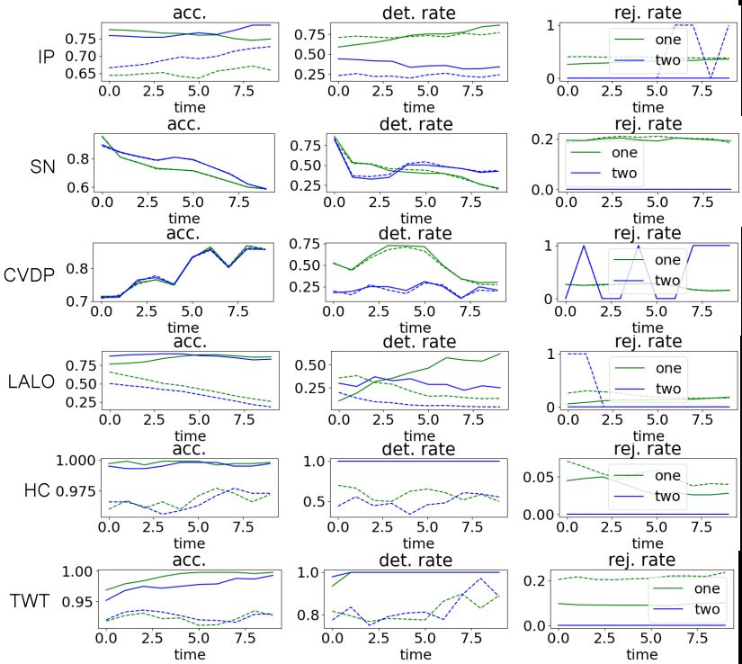
4       F. Cairoli et al.

   The predictor g is an approximate solution and, as such, it can commit safety-critical
prediction errors. Building on [9], we endow the predictive monitor with an error detection
criterion R. This criterion should be able to preemptively identify – and hence, reject –
sequences of observations y where g’s prediction is likely to be erroneous (in which case R
evaluates to 1, 0 otherwise). R should also be optimal in that it has minimal probability
of detection errors. The rationale behind R is that uncertain predictions are more likely
to lead to prediction errors. Hence, rather than operating directly over observations
y, the detector R receives in input a measure of predictive uncertainty of g about y.

Problem 3 (Uncertainty-based error detection under noise and partial observability).
Given an approximate reachability predictor g for the HS and reachability specification
of Problem 2, and a measure of predictive uncertainty ug : Y Hp → D over some
uncertainty domain D, find an optimal error detection rule, Rg∗ : D → {0,1}, that
minimizes the probability
               P ryt ∼Y 1 g(yt)6= 1(Reach(U,st,Hf )) =  6 Rg∗(ug (yt)).

In the above problem, we consider all kinds of prediction errors, but the definition and
approach could be easily adapted to focus on the detection of only e.g., false negatives
(the most problematic errors from a safety-critical viewpoint).
   The general goal of Problems 2 and 3 is to minimize the risk of making mistakes in pre-
dicting reachability and predicting predictions errors, respectively. We are also interested
in establishing probabilistic guarantees on the expected error rate, in the form of predic-
tions regions guaranteed to include the true reachability value with arbitrary probability.

Problem 4 (Probabilistic guarantees). Given the HS and reachability specification of
Problem 2, find a function Γ  :Y Hp →2{0,1}, mapping a sequence of past observations
y into a prediction region for the corresponding reachability value, i.e., a region that
satisfies, for any error probability
                                    level ∈(0,1), the validity property below


                     P ryt ∼Y 1 Reach(U,st,Hf ) ∈Γ yt ≥1−.

Among the maps that satisfy validity, we seek the most efficient one, meaning the one
with the smallest, i.e. less conservative, prediction regions.

3     Methods
In this section, we first describe our learning-based solution to PM under PO (Problem 2).
We then provide background on conformal prediction (CP) and explain how we apply
this technique to endow our reachability predictions and state estimates with probabilis-
tic guarantees (Problem 4). Finally, we illustrate how CP can be used to derive measures
of predictive uncertainty to enable error detection (Problem 3) and active learning.

3.1   Predictive Monitoring under Noise and Partial Observability
There are two natural learning-based approaches to tackle Problem 2 (see Fig. 2):
1. an end-to-end solution that learns a direct mapping from the sequence of past
   measurements yt to the reachability label {0,1}.
2. a two-step solution that combines steps (a) and (b) below: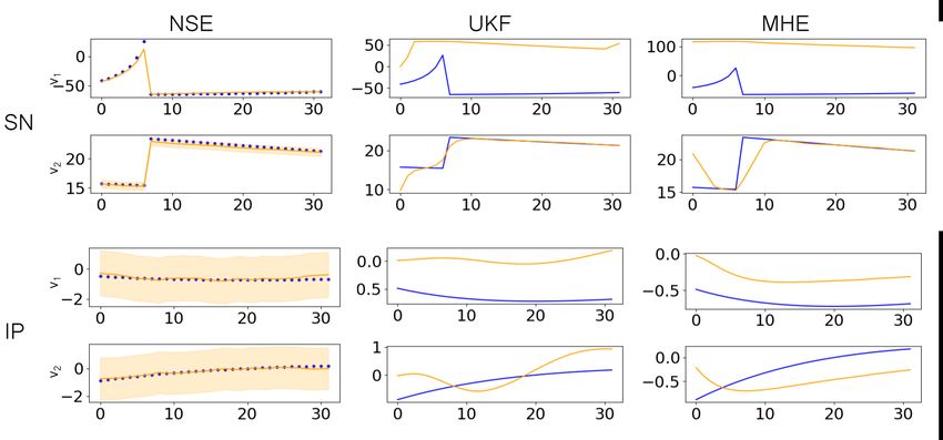
Neural Predictive Monitoring under Partial Observability        5

                           st =(st−Hp ,...,st )

              (2.a) state-estimator                           (2.b) state-classifier
                                                  (1) end-to-end
                          yt =(yt−Hp ,...,yt )                         Reach(U,st ,Hf )

             Fig. 2. Diagram of NSC under noise and partial observability.

 (a) learns a state estimator able to reconstruct the history of full states st =
     (st−Hp ,...,st) from the sequence of measurements yt =(yt−Hp ,...,yt);
 (b) learns a state classifier mapping the sequence of states st to the reachability label
     {0,1};

Dataset Generation. Since we aim to solve the PM problem as one of supervised
learning, the first step is generating a suitable training dataset. For this purpose, we
need reachability oracles to label states s as safe (negative), if ¬Reach(U,s,Hf ), or
unsafe (positive) otherwise. Given that we consider deterministic HS dynamics, we use
simulation (rather than reachability checkers like [12,3,8]) to label the states.
   The reachability of the system at time t depends only on the state of the system
at time t, however, one can decide to exploit more information and make a prediction
based on the previous Hp states. Formally, the generated dataset under full observability
can be expressed as DNP M = {(sit,li)}N                  i     i       i             i
                                            i=1 , where st = (st−Hp ,st−Hp +1 ,...,st ) and
li =1(Reach(U,sit,Hf )) . Under partial observability, we use the (known) observation
function µ:S →Y to build a dataset DP O−NP M made of tuples (yt,st,lt), where yt is
a sequence of noisy observations for st, i.e., such that ∀j ∈{t−Hp,...,t} yj =µ(sj )+wj
and wj ∼W. The distribution of st and yt is determined by the distribution S of the
initial state of the sequences, st−Hp .
   We consider two different distributions: independent, where the initial states st−Hp are
sampled independently, thus resulting in independent state/observation sequences; and
sequential, where states come from temporally correlated trajectories in a sliding-window
fashion. The latter is more suitable for real-world runtime applications, where obser-
vations are received in a sequential manner. On the other hand, temporal dependency
violates the exchangeability property, which affects the theoretical validity guarantees
of CP, as we will soon discuss.
   Starting from DP O−NP M , the two alternative approaches, end-to-end and two-step,
can be developed as follows.

End-to-end solution. We train a one-dimensional convolutional neural net (CNN)
that learns a direct mapping from yt to lt, i.e., we solve a simple binary classification
problem. This approach ignores the sequence of states st. The canonical binary cross-
entropy function can be considered as loss function for the weights optimization process.

Two-step solution. A CNN regressor, referred to as Neural State Estimator (NSE),
is trained to reconstruct the sequence of states ŝt from the sequence of noisy observations
yt. This is combined with, a CNN classifier, referred to as Neural State Classifier (NSC),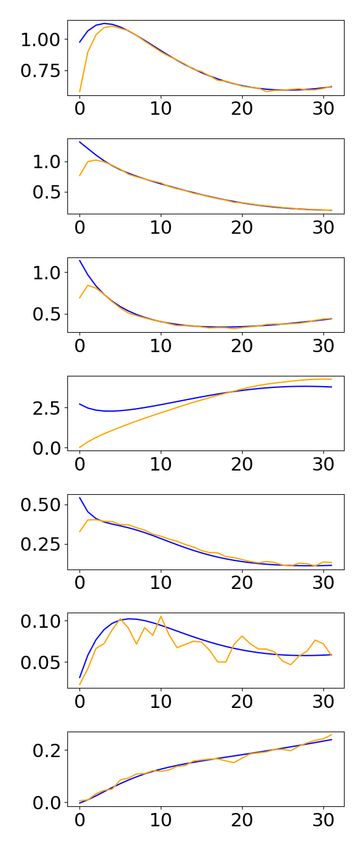
6       F. Cairoli et al.

trained to predict the reachability label lt from the sequence of states st. The mean
square error between the sequences of real states st and the reconstructed ones ŝt is
a suitable loss function for the NSE, whereas for the NSC we use, once again, a binary
cross-entropy function.
   The network resulting from the combination of the the NSE and the NSC maps the
sequence of noisy measurements into the safety label, exactly as required in Problem 2.
However, the NSE inevitably introduces some errors in reconstructing st. Such error
is then propagated when the NSC is evaluated on the reconstructed state, ŝt, as it is
generated from a distribution different from S, affecting the overall accuracy of the
combined net. To alleviate this problem, we introduce a fine-tuning phase in which
the weights of the NSE and the weights of the NSC are updated together, minimizing
the sum of the two respective loss functions. In this phase, the NSC learns to classify
correctly the state reconstructed by the NSE, ŝt, rather than the real state st, so to
improve the task specific accuracy.

Neural State Estimation. The two-step approach has an important additional advantage,
the NSE. In general, any traditional state estimator could have been used. Nevertheless,
non-linear systems make SE extremely challenging for existing approaches. On the
contrary, our NSE reaches very high reconstruction precision (as demonstrated in the
result section). Furthermore, because of the fine-tuning, it is possible to calibrate the
estimates to be more accurate in regions of the state-space that are safety-critical.

3.2   Conformal Prediction for regression and classification
In the following, we provide background on conformal prediction considering a generic
prediction model. Let X be the input space, T be the target space, and define Z =X ×T .
Let Z be the data-generating distribution, i.e., the distribution of the points (x,t)∈Z.
The prediction model is represented as a function f : X → T . For a generic input x,
we denote with t the true target value of x and with t̂ the prediction by f. Test inputs,
whose unknown true target values we aim to predict, are denoted by x∗.
   In our setting of reachability prediction, inputs are observation sequences, target
values are the corresponding reachability values. The data distribution Z is the joint
distribution of observation sequences and reachability values induced by state st−HP ∼S
and iid noise vector wt ∼W Hp .
   Conformal Prediction associates measures of reliability to any traditional supervised
learning problem. It is a very general approach that can be applied across all exist-
ing classification and regression methods [5,34]. CP produces prediction regions with
guaranteed validity, thus satisfying the statistical guarantees illustrated in Problem 4.
Definition 1 (Prediction region). For significance level ∈(0,1) and test input x∗,
the -prediction region for x∗, Γ∗ ⊆T , is a set of target values s.t.
                                   P r (t∗ ∈Γ∗)=1−.                           (2)
                                 (x∗ ,t∗ )∼Z

   The idea of CP is to construct the prediction region by “inverting” a suitable hypothesis
test: given a test point x∗ and a tentative target value t0, we exclude t0 from the prediction
region only if it is unlikely that t0 is the true value for x∗. The test statistic is given by
a so-called nonconformity function (NCF) δ :Z →R, which, given a predictor f and a
point z =(x,t), measures the deviation between the true value t and the corresponding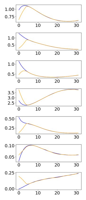
Neural Predictive Monitoring under Partial Observability          7

prediction f(x). In this sense, δ can be viewed as a generalized residual function. In other
words, CP builds the prediction region Γ∗ for a test point x∗ by excluding all targets
t0 whose NCF values areunlikely to follow the NCF distribution of the true targets:
                     Γ∗ = t0 ∈T |P r(x,t)∼Z (δ(x∗,t0)≥δ(x,t))> .                       (3)
The probability term in Eq. 3 is often called p-value. From a practical viewpoint, the
NCF distribution P r(x,t)∼Z (δ(x,t)) cannot be derived in an analytical form, and thus
we use an empirical approximation derived using a sample Zc of Z. This approach
is called inductive CP [24] and Zc is referred to as calibration set.
Remark 1 (Assumptions and guarantees of inductive CP). Importantly, CP prediction
regions have finite-sample validity [5], i.e., they satisfy (2) for any sample of Z (or
reasonable size), and not just asymptotically. On the other hand, CP’s theoretical
guarantees hold under the exchangeability assumption (a “relaxed” version of iid) by
which the joint probability of any sample of Z is invariant to permutations of the
sampled points. Of the two observation distributions discussed in Section 2, we have
that independent observations are exchangeable but sequential ones are not (due to the
temporal dependency). Even though sequential data violate CP’s theoretical validity,
we find that the prediction regions still attain empirical coverage consistent with the
nominal coverage (see results section), that is, the probabilistic guarantees still hold in
practice (as also found in previous work on CP and time-series data [5]).
Validity and Efficiency. CP performance is measured via two quantities: 1) validity
(or coverage), i.e. the empirical error rate observed on a test sample, which should
be as close as possible to the significance level , and 2) efficiency, i.e. the size of the
prediction regions, which should be small. CP-based prediction regions are automatically
valid (under the assumptions of Remark 1), whereas the efficiency depends on the
chosen nonconformity function and thus the underlying model.

CP for classification. In classification, the target space is a discrete set of possible
labels (or classes) T ={`1,...,`c}. We represent the classification model as a function f :
X →[0,1]c mapping inputs into a vector of class likelihoods, such that the predicted class
is the one with the highest likelihood5. Classification is relevant for predictive monitoring
as the reachability predictor of Problem 2 is indeed a binary classifier (T ={0,1}) telling
whether or not an unsafe state can be reached given a sequence of observation.
   The inductive CP algorithm for classification is divided into an offline phase, executed
only once, and an online phase, executed for every test point x∗. In the offline phase
(steps 1–3 below), we train the classifier f and construct the calibration distribution, i.e.,
the empirical approximation of the NCF distribution. In the online phase (steps 4–5),
we derive the prediction region for x∗ using the computed classifier and distribution.
1. Draw sample Z 0 of Z. Split Z 0 into training set Zt and calibration set Zc.
2. Train classifier f using Zt. Use f to define an NCF δ.
3. Construct the calibration distribution by computing, for each zi ∈Zc, the NCF score
    αi =δ(zi).
4. For each label `j ∈T , compute α∗j =δ(x∗,`j ), i.e., the NCF score for x∗ and `j , and
    the associated p-value pj∗:
                           |{zi ∈Zc |αi >α∗j }|    |{zi ∈Zc |αi =α∗j }|+1
                     pj∗ =                      +θ                          ,             (4)
                                 |Zc|+1                     |Zc|+1
 5
     Ties can be resolved by imposing an ordering over the classes.
8         F. Cairoli et al.

    where θ ∈U[0,1] is a tie-breaking random variable.
5. Return the prediction region Γ∗ ={`j ∈T |pj∗ >}.
In defining the NCF δ, we should aim to obtain high δ values for wrong predictions
and low δ values for correct ones. Thus, a natural choice in classification is to define
δ(x,lj ) = 1−f(x)j , where f(x)j is the likelihood predicted by f for class lj . Indeed,
if lj is the true target for x and f correctly predicts lj , then f(x)j is high (the highest
among all classes) and δ(x,lj ) is low; the opposite holds if f does not predict lj .

CP for Regression. In regression we have a continuous target space T ⊆Rn. Thus,
the regression case is relevant for us because our state estimator can be viewed as a
regression model, where T is the state space.
   The CP algorithm for regression is similar to the classification one. In particular,
the offline phase of steps 1–3, i.e., training of regression model f and definition of NCF
δ, is the same (with obviously a different kind of f and δ).
   The online phase changes though, because T is a continuous space and thus, it is
not possible to enumerate the target values and compute for each a p-value. Instead,
we proceed in an equivalent manner, that is, identify the critical value α() of the
calibration distribution, i.e., the NCF score corresponding to a p-value of . The resulting
-prediction region is given by Γ∗ = f(x∗)±α(), where α() is the (1−)-quantile of
the calibration distribution, i.e., the b·(|Zc|+1)c-th largest calibration score6.
   A natural NCF in regression, and the one used in our experiments, is the norm of
the difference between the real and the predicted target value, i.e., δ(x)=||t−f(x)||.

3.3     CP-based quantification of predictive uncertainty

We illustrate how to complement reachability predictions with uncertainty-based error
detection rules, which leverage measures of predictive uncertainty to preemptively
identify the occurrence of prediction errors. Detecting errors efficiently requires a fine
balance between the number of errors accurately prevented and the overall number
of discarded predictions.
   We use two uncertainty measures, confidence and credibility, that are extracted from
the CP algorithm for classification. The method discussed below was first introduced
for NPM [9], but here this is extended to the PO case.

Confidence and credibility. Let us start by observing that, for significance levels
1 ≥2, the corresponding prediction regions are such that Γ 1 ⊆Γ 2 . It follows that,
given an input x∗, if  is lower than all its p-values, i.e.  < minj=1,...,c pj∗, then the
region Γ∗ contains all the labels. As  increases, fewer and fewer classes will have a
p-value higher than . That is, the region shrinks as  increases. In particular, Γ∗ is
empty when ≥maxj=1,...,c pj∗.
   The confidence of a point x∗ ∈X, 1−γ∗, measures how likely is our prediction for
x∗ compared to all other possible classifications (according to the calibration set). It
6
    Such prediction intervals have the same width (α() ) for all inputs. There are techniques
    like [30] that allow to construct intervals with input-dependent widths, which can be
    equivalently applied to our problem.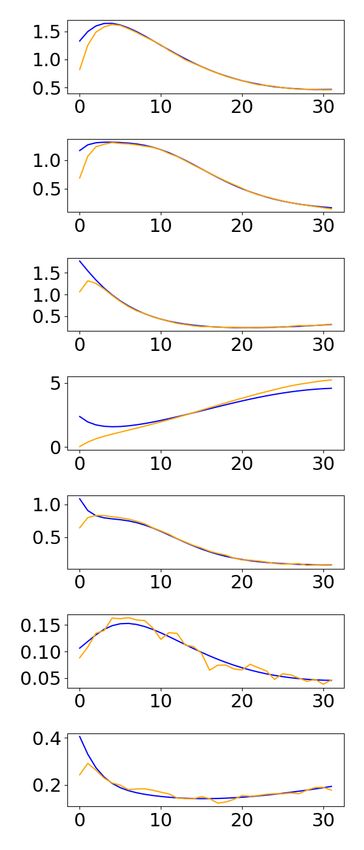
Neural Predictive Monitoring under Partial Observability            9

is computed as one minus the smallest value of  for which the conformal region is
a single label, i.e. the second largest p-value γ∗:
                                  1−γ∗ =sup{1−:|Γ∗|=1}.
    The credibility, c∗, indicates how suitable the training data are to classify that specific
example. In practice, it is the smallest  for which the prediction region is empty, i.e.
the highest p-value according to the calibration set, which corresponds to the p-value
of the predicted class:
                                     c∗ =inf{:|Γ∗|=0}.
    Note that if γ∗ ≤, then the corresponding prediction region Γ∗ contains at most
one class. If both γ∗ ≤ and c∗ > hold, then the prediction region contains exactly one
class, denoted as ˆ`∗, i.e., the one predicted by f. In other words, the interval [γ∗,c∗)
contains all the  values for which we are sure that Γ∗ ={ˆ`∗}. It follows that the higher
1−γ∗ and c∗ are, the more reliable the prediction ˆ`∗ is, because we have an expanded
range [γ∗,c∗) of significance values by which ˆ`∗ is valid. Indeed, in the extreme scenario
where c∗ =1 and γ∗ =0, then Γ∗ ={ˆ`∗} for any value of . This is why, as we will soon
explain, our uncertainty-based rejection criterion relies on excluding points with low
values of 1−γ∗ and c∗. In binary classification problems, each point x∗ has only two
p-values, one for each class, which coincide with c∗ (p-value of the predicted class) and
γ∗ (p-value of the other class).
    Given a reachability predictor g, the uncertainty function ug can be defined as
the function mapping a sequence of observations y∗ into the confidence γ ∗ and the
credibility c∗ of g(y∗), thus ug (y∗)=(γ ∗,c∗). In order to learn a good decision rule to
identify trustworthy predictions, we solve another binary classification problem on the
uncertainty values. In particular, we use a cross-validation strategy to compute values
of confidence and credibility over the entire calibration set, as it is not used to train the
classifier, and label each point as 0 if it is correctly classified by the predictor and as 1
if it is misclassified. We then train a Support Vector Classifier (SVC) that automatically
learns to distinguish points that are misclassified from points that are correctly classified
based on the values of confidence and credibility. In particular, we choose a simple
linear classifier as it turns out to perform satisfactorily well, especially on strongly
unbalanced datasets. Nevertheless, other kinds of classifiers can be applied as well.
    To summarize, given a predictor g and a new sequence of observations y∗, we
obtain a prediction about its safety, g(y∗)= l̂∗, and a quantification of its uncertainty,
u∗ = ug (y∗) = (γ ∗,c∗). If we feed u∗ to the rejection rule Rg we obtain a prediction
about whether or not the prediction of g about y∗ can be trusted.

3.4   Active Learning (AL)

NPM depends on two related learning problems: the reachabiliy predictor g and the
rejection rule Rg . We leverage the uncertainty-aware active learning solution presented
in [10], where the re-training points are derived by first sampling a large pool of
unlabeled data, and then considering only those points where the current predictor g is
still uncertain, i.e. those points which are rejected by our rejection rule Rg . A fraction
of the labeled samples is added to the training set, whereas the remaining part is added
to the calibration set, keeping the training/calibration ratio constant. As a matter of
fact, a principled criterion to select the most informative samples would benefit both
10      F. Cairoli et al.

the accuracy and the efficiency of the method, as the size of the calibration set affects
the runtime efficiency of the error detection rule.
   The addition of such actively selected points results in a shift of the data generating
distribution, that does not match anymore the distribution of the test samples. This
implies that the theoretical guarantees of CP are lost. However, as we will show in
the experiments, AL typically results in an empirical increase of the coverage, i.e., in
even stronger probabilistic guarantees. The reason is that AL is designed to improve
on poor predictions, which, as such, have prediction regions more likely to miss the
true value. Improving such poor predictions thus directly cause an increased coverage
(assuming that the classifier remains accurate enough on the inputs prior to AL).

4     Experimental Evaluation
We evaluate both end-to-end and two-step approaches under PO on six benchmarks
of cyber-physical systems with dynamics presenting a varying degree of complexity and
with a variety of observation functions. We include white Gaussian noise to introduce
stochasticity in the observations.

4.1   Case Studies
– IP: classic two-dimensional non-linear model of an Inverted Pendulum on a cart.
  Given a state s=(s1,s2), we observe a noisy measure of the energy of the system
  y =s2/2+cos(s1)−1+w, where w ∼N (0,0.005). Unsafe region U ={s:|s1|≥π/6}.
  Hp =1, Hf =5.
– SN: a two-dimensional non-linear model of the Spiking Neuron action potential.
  Given a state s = (s1,s2) we observe a noisy measure of s2, y = s2 + w, with
  w ∼N (0,0.1). Unsafe region U ={s:s1 ≤−68.5}. Hp =4, Hf =16.
– CVDP: a four-dimensional non-linear model of the Coupled Van Der Pol oscilla-
  tor [15], modeling two coupled oscillators. Given a state s=(s1,s2,s3,s4) we observe
  y =(s1,s3)+w, with w ∼N (0,0.01·I2). Unsafe region U ={s:s2 ≥2.75∧s2 ≥2.75}.
  Hp =8, Hf =7.
– LALO: the seven-dimensional non-linear Laub Loomis model [15] of a class
  of enzymatic activities. Given a state s = (s1, s2, s3, s4, s5, s6, s7) we observe
  y = (s1,s2,s3,s5,s6,s7)+w, with w ∼ N (0,0.01·I6). Unsafe region U = {s : s4 ≥ 4.5}.
  Hp =5, Hf =20.
– TWT: a three-dimensional non-linear model of a Triple Water Tank. Given a
  state s = (s1,s2,s3) we observe y = s + w, with w ∼ N (0,0.01 · I3). Unsafe region
            3
  U ={s:∨i=1   si ∈
                  6 [4.5,5.5]}. Hp =1, Hf =1.
– HC: the 28-dimensional linear model of an Helicopter controller. We observe only
  the altitude, i.e. y =s8 +w, with w ∼N (0,1). Unsafe region U ={s:s8
Neural Predictive Monitoring under Partial Observability 11
version), (3) train the NPM (either end-to-end or two-step), (4) train the CP-based
error detection rules, (5) perform active learning and (6) evaluate both the initial and
the active NPM on a test set. From here on, we call initial setting the one with no
active learning involved. The technique is fully implemented in Python7. In particu-
lar, PyTorch [25] is used to craft, train and evaluate the desired CNN architectures.
Details about the CNN architectures and the settings of the optimization algorithm
are described in Appendix D. The source code for all the experiments can be found
at the following link: https://github.com/francescacairoli/Stoch_NSC.git
Datasets. For each case study we generate both an independent and a sequential dataset.
– Independent: the train set consists of 50K independent sequences of states of length
32, the respective noisy measurements and the reachability labels. The calibration
and test set contains respectively 8.5K and 10K samples.
– Sequential: for the train set, 5K states are randomly sampled. From each of these states
we simulate a long trajectory. From each long trajectory we obtain 100 sub-trajectories
of length 32 in a sliding window fashion. The same procedure is applied to the test
and calibration set, where the number of initial states is respectively 1K and 850.
Data are scaled to the interval [−1,1] to avoid sensitivity to different scales. While the
chosen datasets are not too large, our approach would work well even with smaller
datasets, resulting however in lower accuracy and higher uncertainty. In these cases,
our proposed uncertainty-based active learning would represent the go-to solution as
is designed for situations where data collection is particularly expensive.
Computational costs. NPM is designed to work at runtime in safety-critical applications,
which translates in the need of high computational efficiency together with high reliability.
The time needed to generate the dataset and to train both methods does not affect the
runtime efficiency of the NPM, as it is performed only once (offline). Once trained, the
time needed to analyse the reachability of the current sequence of observations is the
time needed to evaluate one (or two) CNN, which is almost negligible (in the order of
microseconds on GPU). On the other hand, the time needed to quantify the uncertainty
depends on the size of the calibration set. This is one of the reasons that make active
learning a preferable option, as it adds only the most significant points to the dataset.
It is important to notice that the percentage of points rejected, meaning points with
predictions estimated to be unreliable, affects considerably the runtime efficiency of the
methods. Therefore, we seek a trade-off between accuracy and runtime efficiency. Training
the end-to-end approach takes around 15 minutes. Training the two-step approach takes
around 40 minutes: 9 for the NSE, 11 for the NSC and 20 minutes for the fine-tuning.
Making a single prediction takes around 7×10⁻⁷ seconds in the end-to-end scenario and
9×10⁻⁷ seconds in the two-step scenario. Training the SVC takes from 0.5 to 10 seconds,
whereas computing values of confidence and credibility for a single point takes from 0.3
to 2 ms. Actively query new data from a pool of 50K samples takes around 5 minutes.
Performance measures. The measures used to quantify the overall performance of the
NPM under PO (both end-to-end and two-step) are: the accuracy of the reachability
predictor, the error detection rate and the rejection rate. We seek high accuracies and
7
The experiments were performed on a computer with a CPU Intel x86, 24 cores and a
128GB RAM and 15GB of GPU Tesla V100.12 F. Cairoli et al.
detection rates without being overly conservative, meaning keeping a rejection rate as
low as possible. We also check if and when the statistical guarantees are met empirically,
via values of coverage and efficiency. We analyse and compare the performances of
NPM under PO on different configurations: an initial and active configuration for
independent states and a temporally correlated (sequential) configuration. Additionally,
we test the method for anomaly detection.
4.3 Results
Initial setting. Table 1 compares the performances of the two approaches to PO-NPM
via predictive accuracy, detection rate, i.e. the percentage of prediction errors, either
false-positives (FP) or false-negatives (FN), recognized by the error detection rule, and
the overall rejection over the test set. We can observe how both methods work well
despite PO, i.e., they reach extremely high accuracies and high detection rate. However,
the two-step approach seems to behave slightly better than the end-to-end. As a matter
of fact, accuracy is almost always greater than 99% with a detection rate close to 100.00.
The average rejection rate is around 11% in the end-to-end scenario, and reduces to
9% in the two-step scenario, making the latter less conservative ant thus more efficient
from a computational point of view. These results come with no surprise, because,
compared to the end-to-end one, the two-step approach leverages more information
available in the dataset for training, that is the exact sequence of states.
End-to-end Two-step
Model Acc. Det. FN FP Rej. Acc. Det. FN FP Rej.
SN 97.72 94.30 79/88 136/140 11.30 97.12 95.49 53/54 222/234 19.98
IP 96.27 93.48 148/155 153/167 27.32 98.42 91.14 81/91 63/66 10.01
CVDP 99.19 100.00 30/30 51/51 5.75 99.68 100.00 17/17 15/15 3.51
TWT 98.93 95.51 18/20 67/69 7.45 98.93 96.26 52/56 51/51 10.46
LALO 98.88 99.11 66/66 45/46 7.39 99.24 100.00 52/52 24/24 6.11
HC 99.63 100.00 19/19 15/15 8.47 99.84 100.00 8/8 8/8 4.03
Table 1. Initial results: Acc. is the accuracy of the PO-NPM, Det. the detection rate, Rej.
the rejection rate of the error detection rule and FN (FP) is the number of detected false
negative (positive) errors.
Benefits of active learning. Table 2 presents the results after one iteration of active
learning. Additional data were selected from a pool of 50K points, using the error
detection rule as query strategy. We observe a slight improvement in the performance,
mainly reflected in higher detection rates and smaller rejection rates, with an average
that reduces to 8% for the end-to-end and to 6% for the two-step.
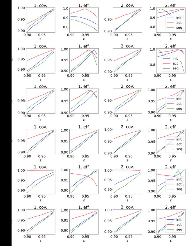
Probabilisic guarantees. In our experiments, we measured the efficiency as the percentage
of singleton prediction regions over the test set. Table 3 compares the empirical coverage
and the efficiency of the CP prediction regions in the initial and active scenario for
both the end-to-end and two-step classifiers. The confidence level is set to (1−)=95%.
Fig. 6 in Appendix C shows coverage and efficiency for different significance levels
(ranging from 0.01 to 0.1). CP provides theoretical guarantees on the validity, meaningNeural Predictive Monitoring under Partial Observability 13
End-to-end Two-step
Model Acc. Det. FN FP Rej. Acc. Det. FN FP Rej.
SN 98.06 94.87 81/88 104/107 9.80 98.41 100.00 55/55 104/104 12.00
IP 99.47 87.91 150/166 119/140 15.44 98.75 92.86 63/69 52/56 7.72
CVDP 99.10 95.55 43/46 43/44 4.81 99.69 100.00 19/19 12/12 2.48
TWT 99.04 100.00 45/45 62/62 10.45 99.07 94.62 44/49 44/44 6.20
LALO 98.79 96.69 87/90 30/31 6.88 99.27 100.00 40/40 33/33 4.28
HC 99.86 100.00 5/5 9/9 2.35 99.79 100.00 17/17 4/4 2.73
Table 2. Active results (1 iteration): Acc. is the accuracy of the PO-NPM, Det. the
detection rate, Rej. the rejection rate of the error detection rule and FN (FP) is the number
of detected false negative (positive) errors.
empirical coverage matching the expected one of 95%, only in the initial setting. As
a matter of fact, with active learning we modify the data-generating distribution of the
training and calibration sets, while the test set remains the same, i.e., sampled from
the original data distribution. As a result, we observe (Table 3) that both methods in
the initial setting are valid. In the active scenario, even if theoretical guarantees are lost,
we obtain both better coverage and higher efficiency. This means that the increased
coverage is not due to a more conservative predictor but to an improved accuracy.
End-to-end Two-step
initial active initial active
Model Cov. Eff. Cov. Eff. Cov. Eff. Cov. Eff.
SN 95.12 95.70 97.19 98.50 94.80 99.54 97.32 98.37
IP 95.30 89.31 96.60 99.62 94.85 94.92 97.28 97.88
CVDP 95.73 95.73 98.00 98.02 95.63 95.63 98.31 98.34
TWT 96.43 96.43 99.99 97.26 96.60 96.97 99.66 97.20
LALO 94.59 94.61 97.28 98.52 94.66 94.66 97.48 97.55
HC 95.03 95.03 97.65 97.65 94.97 94.97 97.69 97.69
Table 3. Coverage and efficiency for both the approaches to PO-NPM. Initial results are
compared with results after one active learning iteration. Expected coverage 95%.
Table 4 shows values of coverage and efficiency for the two separate steps (state
estimation and reachability prediction) of the two-step approach. Recall that the
efficiency in the case of regression, and thus of state estimation, is given by the volume
of the prediction region. So, the smaller the volume, the more efficient the regressor.
The opposite holds for classifiers, where a large value of efficiency means tight prediction
regions. It is interesting to observe how active learning makes the NSC reach higher
coverages at the cost of more conservative prediction regions (lower efficiency), whereas
the NSE coverage is largely unaffected by active learning (except for TWT). Reduction
in NSC efficiency, differently from the two-step combined approach, is likely due to
an adaptation of the method to deal with and correct noisy estimates. Such behaviour
suggests that the difficulty in predicting the reachability of a certain state is independent
of how hard it is to reconstruct that state8.
8
We select re-training points based on the uncertainty of the reachability predictor; if the SE
performed badly on those same points, re-training would have led to a higher SE accuracy
and hence, increased coverage.14 F. Cairoli et al.
NSC NSE
initial active initial active
Model Cov. Eff. Cov. Eff. Cov. Eff. Cov. Eff.
SN 94.82 99.51 97.23 90.12 94.49 1.361 95.18 1.621
IP 94.51 99.69 97.23 91.63 94.65 3.064 95.44 3.233
CVDP 95.60 95.64 98.25 98.32 95.37 0.343 96.40 0.358
TWT 96.68 96.98 98.72 95.61 95.07 0.770 100.00 1.366
LALO 94.88 98.18 98.01 80.86 95.29 0.6561 95.36 0.8582
HC 94.67 94.74 97.33 99.12 94.50 12.44 94.58 12.464
Table 4. Coverage and efficiency for the two steps of the two-step approach. NSC is a classifier,
whereas NSE is a regressor. Initial results are compared with results after one active learning
iteration. Expected coverage 95%.
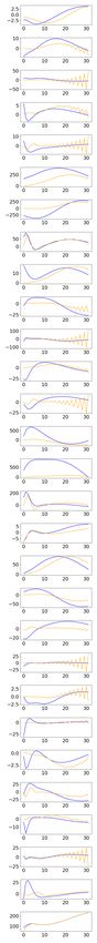
State estimator. We compare the performances of the NSE with two traditional state
estimation techniques: Unscented Kalman Filters9 (UKF) [35] and Moving Horizon
Estimation10 (MHE) [1]. In particular, for each point in the test set we compute the
relative error given by the norm of the difference between the real and reconstructed
state trajectories divided by the maximum range of state values. The results, presented
in full in Appendix E, show how our neural network-based state estimator significantly
outperforms both UKF and MHE in our case studies. Moreover, unlike the existing SE
approaches, our state estimates come with a prediction region that provides probabilistic
guarantees on the expected reconstruction error, as shown in Fig. 3.
Fig. 3. Comparison of different state estimators on a state of the SN (top) and IP (bottom)
model. Blue is the exact state sequence, orange is the estimated one.
Sequential data. All the results presented so far consider a dataset DP O−NP M of
observation sequences generated by independently sampled initial states. However, we are
interested in applying NPM at runtime to systems that are evolving in time. States will
thus have a temporal correlation, meaning that we lose the exchangeability requirement
9
pykalman library: https://pykalman.github.io/
10
do-mpc library: https://www.do-mpc.com/en/latest/Neural Predictive Monitoring under Partial Observability 15
behind the theoretical validity of CP regions. Table 5 shows the performance of predictor
and error detection trained and tested on sequential data. In general, accuracy and
detection rates are still very high (typically above 95%), but the results are on average
worse than the independent counterpart. The motivation could be two-fold: on one side,
it is reasonable to assume that a recurrent neural net would perform better on sequential
data, compared to CNN, on the other, the samples contained in the sequential dataset
are strongly correlated and thus they may cover only poorly the state space. The table
also shows values of coverage and efficiency of both the end-to-end and the two-step
approach. Even if theoretical validity is lost, we still observe empirical coverages that
match the nominal value of 95%, i.e., the probabilistic guarantees are satisfied in practice.
End-to-end Two-step
Model Acc. Det. Rej. Cov. Eff. Acc. Det. Rej. Cov Eff.
SN 94.96 85.83 19.74 93.93 97.73 90.37 81.93 26.59 95.01 88.66
IP 94.17 91.08 31.74 95.31 84.32 91.47 98.01 30.81 95.23 90.23
CVDP 98.97 99.12 7.97 94.88 94.92 98.33 98.20 9.89 94.89 95.19
TWT 96.95 95.33 16.84 93.42 94.52 95.74 92.72 23.52 93.60 96.16
LALO 98.99 97.75 7.18 95.93 97.08 99.26 100.00 5.37 95.78 95.80
HC 99.57 100.00 3.89 94.29 94.29 99.64 97.22 3.84 94.51 94.52
Table 5. Sequential results: Acc. is the accuracy of the PO-NPM, Det. the detection rate,
Rej. the rejection rate, Cov. the CP coverage and Eff. the CP efficiency.
Anomaly detection. The data-generating distribution at runtime is assumed to coincide
with the one used to generate the datasets. However, in practice, such distribution is
typically unknown and subject to runtime deviations. Thus, we are interested to observe
how the sequential PO-NPM behave when an anomaly takes place. In our experiments,
we model an anomaly as an increase in the variance of the measurement noise, i.e.
W 0 = N (0,0.25·I). Fig. 4 compares the performances with VS without anomaly on
a single case study (the other case studies are shown in Appendix B). We observe that
the anomaly causes a drop in accuracy and error detection rate, which comes with an
increase in the number of predictions rejected because deemed to be unreliable. These
preliminary results show how an increase in the NPM rejection rate could be used as
a significant measure to preemptively detect runtime anomalies.
Fig. 4. Anomaly detection (TWT model). Dashed lines denotes the performances on
observations with anomaly in the noise. Blue is for the two-step approach, green for the
end-to-end.16 F. Cairoli et al.
5 Related work
Our approach extends and generalize neural predictive monitoring [9,10] to work under
partial observability. To our knowledge, the only existing work to focus on PM and PO
is [13], which combines Bayesian estimation with pre-computed reach sets to reduce
the runtime overhead. While their reachability bounds are certified, no correctness
guarantees can be established for the estimation step. Our work instead provides
probabilistic guarantees as well as techniques for preemptive error detection. A related
but substantially different problem is to verify signals with observation gaps using state
estimation to fill the gaps [33,20].
In [28] a model-based approach to predictive runtime verification is presented. How-
ever, PO and computational efficiency are not taken into account. A problem very
similar to ours is addressed in [19], but for a different class of systems (MDPs).
Learning-based approaches for reachability prediction of hybrid and stochastic systems
include [11,26,14,31,36,16]. Of these, [36] develop, akin to our work, error detection
techniques, but using neural network verification methods [17]. Such verification meth-
ods, however, do not scale well on large models and support only specific classes of
neural networks. On the opposite, our uncertainty-based error detection can be applied
to any ML-based predictive monitor. Learning-based PM approaches for temporal
logic properties [29,22] typically learn a time-series model from past observations and
then use such model to infer property satisfaction. In particular, [29] provide (like
we do) guaranteed prediction intervals, but (unlike our method) they are limited to
ARMA/ARIMA models. Ma et al [22] use uncertainty quantification with Bayesian
RNNs to provide confidence guarantees. However, these models are, by nature, not
well-calibrated (i.e., the model uncertainty does not reflect the observed one [21]),
making the resulting guarantees not theoretically valid11.
PM is at the core of the Simplex architecture [32,18] and recent extensions thereof [27,23],
where the PM component determines when to switch to the fail-safe controller to prevent
imminent safety violations. In this context, our approach can be used to guarantee
arbitrarily small probability of wrongly failing to switch.
6 Conclusion
We presented an extension of the Neural Predictive Monitoring [10] framework to work
under the most realistic settings of noise and partially observability. We proposed two
alternative solution strategies: an end-to-end solution, predicting reachability directly
from raw observations, and a two-step solution, with an intermediate state estimation
step. Both methods produce extremely accurate predictions, with the two-step approach
performing better overall than the end-to-end version, and further providing accurate
reconstructions of the true state. The online computational cost is negligible, making this
method suitable for runtime applications. The method is equipped with an error detection
rule to prevent reachability prediction errors, as well as with prediction regions providing
probabilistic guarantees. We demonstrated that error detection can be meaningfully
used for active learning, thereby improving our models on the most uncertain inputs.
11
The authors develop a solution for Bayesian RNNs calibration, but such solution in turn
is not guaranteed to produce well-calibrated models.Neural Predictive Monitoring under Partial Observability 17
As future work, we plan to extend this approach to fully stochastic models, inves-
tigating the use of deep generative models for state estimation. We will further explore
the use of recurrent or attention-based architectures in place of convolutional ones to
improve performance for sequential data.
References
1. Allan, D.A., Rawlings, J.B.: Moving horizon estimation. In: Handbook of Model Predictive
Control, pp. 99–124. Springer (2019)
2. Allgöwer, F., Badgwell, T.A., Qin, J.S., Rawlings, J.B., Wright, S.J.: Nonlinear predictive
control and moving horizon estimation—an introductory overview. Advances in control
pp. 391–449 (1999)
3. Althoff, M., Grebenyuk, D.: Implementation of interval arithmetic in CORA 2016. In:
Proc. of the 3rd International Workshop on Applied Verification for Continuous and
Hybrid Systems (2016)
4. Alur, R.: Principles of cyber-physical systems. MIT Press (2015)
5. Balasubramanian, V., Ho, S.S., Vovk, V.: Conformal prediction for reliable machine
learning: theory, adaptations and applications. Newnes (2014)
6. Bartocci, E., Deshmukh, J., Donzé, A., Fainekos, G., Maler, O., Ničković, D., Sankara-
narayanan, S.: Specification-based monitoring of cyber-physical systems: a survey on theory,
tools and applications. In: Lectures on Runtime Verification, pp. 135–175. Springer (2018)
7. Bengio, Y., CA, M.: Rmsprop and equilibrated adaptive learning rates for nonconvex
optimization. corr abs/1502.04390 (2015)
8. Bogomolov, S., Forets, M., Frehse, G., Potomkin, K., Schilling, C.: JuliaReach: a toolbox
for set-based reachability. In: Proceedings of the 22nd ACM International Conference
on Hybrid Systems: Computation and Control. pp. 39–44 (2019)
9. Bortolussi, L., Cairoli, F., Paoletti, N., Smolka, S.A., Stoller, S.D.: Neural predictive moni-
toring. In: International Conference on Runtime Verification. pp. 129–147. Springer (2019)
10. Bortolussi, L., Cairoli, F., Paoletti, N., Smolka, S.A., Stoller, S.D.: Neural predictive
monitoring and a comparison of frequentist and bayesian approaches. International
Journal on Software Tools for Technology Transfer, to appear (2021)
11. Bortolussi, L., Milios, D., Sanguinetti, G.: Smoothed model checking for uncertain
continuous-time Markov chains. Information and Computation 247, 235–253 (2016)
12. Chen, X., Ábrahám, E., Sankaranarayanan, S.: Flow*: An analyzer for non-linear hybrid
systems. In: International Conference on Computer Aided Verification. pp. 258–263.
Springer (2013)
13. Chou, Y., Yoon, H., Sankaranarayanan, S.: Predictive runtime monitoring of vehicle
models using bayesian estimation and reachability analysis. In: Intl. Conference on
Intelligent Robots and Systems (IROS) (2020)
14. Djeridane, B., Lygeros, J.: Neural approximation of PDE solutions: An application to
reachability computations. In: Proceedings of the 45th IEEE Conference on Decision
and Control. pp. 3034–3039. IEEE (2006)
15. Ernst, G., Arcaini, P., Bennani, I., Donze, A., Fainekos, G., Frehse, G., Mathesen,
L., Menghi, C., Pedrinelli, G., Pouzet, M., et al.: Arch-comp 2020 category report:
Falsification. EPiC Series in Computing (2020)
16. Granig, W., Jakšić, S., Lewitschnig, H., Mateis, C., Ničković, D.: Weakness monitors
for fail-aware systems. In: International Conference on Formal Modeling and Analysis
of Timed Systems. pp. 283–299. Springer (2020)
17. Ivanov, R., Weimer, J., Alur, R., Pappas, G.J., Lee, I.: Verisig: verifying safety properties
of hybrid systems with neural network controllers. In: Proceedings of the 22nd ACM
International Conference on Hybrid Systems: Computation and Control. pp. 169–178 (2019)18 F. Cairoli et al.
18. Johnson, T.T., Bak, S., Caccamo, M., Sha, L.: Real-time reachability for verified simplex
design. ACM Transactions on Embedded Computing Systems (TECS) 15(2), 1–27 (2016)
19. Junges, S., Torfah, H., Seshia, S.A.: Runtime monitors for markov decision processes. In:
International Conference on Computer Aided Verification. pp. 553–576. Springer (2021)
20. Kalajdzic, K., Bartocci, E., Smolka, S.A., Stoller, S.D., Grosu, R.: Runtime verification
with particle filtering. In: International Conference on Runtime Verification. pp. 149–166.
Springer (2013)
21. Kuleshov, V., Fenner, N., Ermon, S.: Accurate uncertainties for deep learning using
calibrated regression. In: International Conference on Machine Learning. pp. 2796–2804.
PMLR (2018)
22. Ma, M., Stankovic, J.A., Bartocci, E., Feng, L.: Predictive monitoring with logic-calibrated
uncertainty for cyber-physical systems. CoRR abs/2011.00384v2 (2020)
23. Mehmood, U., Stoller, S.D., Grosu, R., Roy, S., Damare, A., Smolka, S.A.: A distributed
simplex architecture for multi-agent systems. arXiv preprint arXiv:2012.10153 (2020)
24. Papadopoulos, H.: Inductive conformal prediction: Theory and application to neural
networks. In: Tools in artificial intelligence. InTech (2008)
25. Paszke, A., Gross, S., Chintala, S., Chanan, G., Yang, E., DeVito, Z., Lin, Z., Desmaison,
A., Antiga, L., Lerer, A.: Automatic differentiation in pytorch. In: NIPS-W (2017)
26. Phan, D., Paoletti, N., Zhang, T., Grosu, R., Smolka, S.A., Stoller, S.D.: Neural state
classification for hybrid systems. In: International Symposium on Automated Technology
for Verification and Analysis (ATVA 2018). pp. 422–440. Springer (2018)
27. Phan, D.T., Grosu, R., Jansen, N., Paoletti, N., Smolka, S.A., Stoller, S.D.: Neural
simplex architecture. In: NASA Formal Methods Symposium. pp. 97–114. Springer (2020)
28. Pinisetty, S., Jéron, T., Tripakis, S., Falcone, Y., Marchand, H., Preoteasa, V.: Predictive
runtime verification of timed properties. Journal of Systems and Software 132, 353–365
(2017)
29. Qin, X., Deshmukh, J.V.: Predictive monitoring for signal temporal logic with probabilistic
guarantees. In: Proceedings of the 22nd ACM International Conference on Hybrid
Systems: Computation and Control. pp. 266–267. ACM (2019)
30. Romano, Y., Patterson, E., Candès, E.J.: Conformalized quantile regression. arXiv
preprint arXiv:1905.03222 (2019)
31. Royo, V.R., Fridovich-Keil, D., Herbert, S., Tomlin, C.J.: Classification-based approximate
reachability with guarantees applied to safe trajectory tracking. arXiv preprint
arXiv:1803.03237 (2018)
32. Sha, L., et al.: Using simplicity to control complexity. IEEE Software 18(4), 20–28 (2001)
33. Stoller, S.D., Bartocci, E., Seyster, J., Grosu, R., Havelund, K., Smolka, S.A., Zadok,
E.: Runtime verification with state estimation. In: International conference on runtime
verification. pp. 193–207. Springer (2011)
34. Vovk, V., Gammerman, A., Shafer, G.: Algorithmic learning in a random world. Springer
Science & Business Media (2005)
35. Wan, E.A., Van Der Merwe, R.: The unscented kalman filter for nonlinear estimation. In:
Proceedings of the IEEE 2000 Adaptive Systems for Signal Processing, Communications,
and Control Symposium (Cat. No. 00EX373). pp. 153–158. Ieee (2000)
36. Yel, E., Carpenter, T.J., Di Franco, C., Ivanov, R., Kantaros, Y., Lee, I., Weimer, J., Bezzo,
N.: Assured runtime monitoring and planning: Toward verification of neural networks for
safe autonomous operations. IEEE Robotics & Automation Magazine 27(2), 102–116 (2020)You can also read