National Forest Inventories capture the multifunctionality of managed forests in Germany
←
→
Page content transcription
If your browser does not render page correctly, please read the page content below

Simons et al. Forest Ecosystems     (2021) 8:5
https://doi.org/10.1186/s40663-021-00280-5

 RESEARCH                                                                                                                                           Open Access

National Forest Inventories capture the
multifunctionality of managed forests in
Germany
Nadja K. Simons1,2* , María R. Felipe-Lucia3,4, Peter Schall3, Christian Ammer5,6, Jürgen Bauhus7, Nico Blüthgen8,
Steffen Boch9,10, François Buscot11,12, Markus Fischer9, Kezia Goldmann11, Martin M. Gossner13,14, Falk Hänsel15,
Kirsten Jung16, Peter Manning17, Thomas Nauss15, Yvonne Oelmann18, Rodica Pena6,19,20, Andrea Polle6,20,
Swen C. Renner21, Michael Schloter22,23, Ingo Schöning24, Ernst-Detlef Schulze24, Emily F. Solly24,25,
Elisabeth Sorkau18, Barbara Stempfhuber22, Tesfaye Wubet12,26, Jörg Müller27,28, Sebastian Seibold1,29 and
Wolfgang W. Weisser1

  Abstract
  Background: Forests perform various important ecosystem functions that contribute to ecosystem services. In
  many parts of the world, forest management has shifted from a focus on timber production to multi-purpose
  forestry, combining timber production with the supply of other forest ecosystem services. However, it is unclear
  which forest types provide which ecosystem services and to what extent forests primarily managed for timber
  already supply multiple ecosystem services. Based on a comprehensive dataset collected across 150 forest plots in
  three regions differing in management intensity and species composition, we develop models to predict the
  potential supply of 13 ecosystem services. We use those models to assess the level of multifunctionality of
  managed forests at the national level using national forest inventory data.
  Results: Looking at the potential supply of ecosystem services, we found trade-offs (e.g. between both bark
  beetle control or dung decomposition and both productivity or soil carbon stocks) as well as synergies (e.g.
  for temperature regulation, carbon storage and culturally interesting plants) across the 53 most dominant
  forest types in Germany. No single forest type provided all ecosystem services equally. Some ecosystem
  services showed comparable levels across forest types (e.g. decomposition or richness of saprotrophs), while
  others varied strongly, depending on forest structural attributes (e.g. phosphorous availability or cover of
  edible plants) or tree species composition (e.g. potential nitrification activity). Variability in potential supply of
  ecosystem services was only to a lesser extent driven by environmental conditions. However, the geographic
  variation in ecosystem function supply across Germany was closely linked with the distribution of main tree
  species.
  (Continued on next page)

* Correspondence: nadja.simons@tu-darmstadt.de
1
 Terrestrial Ecology Research Group, Technische Universität München,
Hans-Carl-von-Carlowitz-Platz 2, 85354 Freising, Germany
2
 Present address: Ecological Networks, Technische Universität Darmstadt,
Schnittspahnstraße 3, 64287 Darmstadt, Germany
Full list of author information is available at the end of the article

                                       © The Author(s). 2021 Open Access This article is licensed under a Creative Commons Attribution 4.0 International License,
                                       which permits use, sharing, adaptation, distribution and reproduction in any medium or format, as long as you give
                                       appropriate credit to the original author(s) and the source, provide a link to the Creative Commons licence, and indicate if
                                       changes were made. The images or other third party material in this article are included in the article's Creative Commons
                                       licence, unless indicated otherwise in a credit line to the material. If material is not included in the article's Creative Commons
                                       licence and your intended use is not permitted by statutory regulation or exceeds the permitted use, you will need to obtain
                                       permission directly from the copyright holder. To view a copy of this licence, visit http://creativecommons.org/licenses/by/4.0/.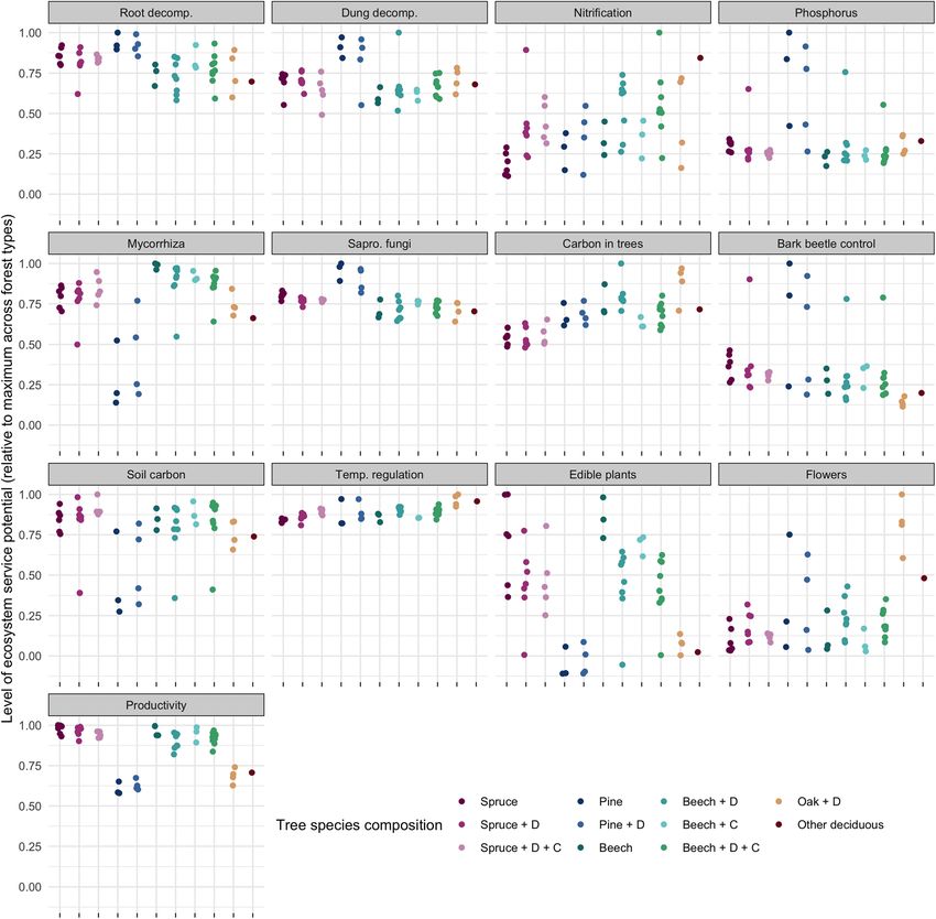
Simons et al. Forest Ecosystems   (2021) 8:5                                                                     Page 2 of 19

 (Continued from previous page)
 Conclusions: Our results show that forest multifunctionality is limited to subsets of ecosystem services. The
 importance of tree species composition highlights that a lack of multifunctionality at the stand level can be
 compensated by managing forests at the landscape level, when stands of complementary forest types are
 combined. These results imply that multi-purpose forestry should be based on a variety of forest types
 requiring coordinated planning across larger spatial scales.
 Keywords: Ecosystem processes and services, Forest management, Structural diversity, Tree species composition,
 Trade-offs and synergies, Forest productivity

Background                                                       et al. 2018). Here, we model the potential supply of eco-
Forests supply multiple regulating, material and non-            system services independently of their actual use or de-
material ecosystem services, i.e. nature’s contributions to      mand (i.e. ecosystem-function multifunctionality) based
people (IPBES 2019), including timber and other non-             on forest attributes such as stand density or tree species
timber products, wild food, carbon sequestration,                composition and other abiotic variables collected across
groundwater recharge, flood regulation, protection from          a range of forest plots in Germany. Ecosystem services
soil erosion, recreational opportunities and habitat             which are mainly driven by demand or (cascading) uses,
provision (Bauhus et al. 2010; Gamfeldt et al. 2013;             such as tourism, long-term climate change mitigation or
Miura et al. 2015; Mori 2017; van der Plas et al. 2017;          replacement of fossil fuels, were not included as data
Storch et al. 2018). Both national (BMELV 2011) and              were not available at the relevant local scales. We use
international (FAO 2013) policy guidelines call for new          those models (also termed ‘production functions’ (Nel-
strategies in forest management, i.e. multi-purpose for-         son et al. 2009; Tallis and Polasky 2011)) to predict the
estry, to deliver as many of these ecosystem services as         potential supply of forest ecosystems across Germany,
possible simultaneously. Yet, the major goal in managed          using data from the National Forest Inventory (NFIs).
forests is typically the production of timber and other          NFIs provide standardized values for forest attributes
wood products, which provide the main or only source             and have long been used to assess the success of forest
of income for forestry. In addition, it is likely that not all   management strategies (Vidal et al. 2016a; Vidal et al.
ecosystem services can be maximized simultaneously,              2016b) and have been explored for assessments of eco-
due to trade-offs between different services (van der Plas       system services or their underlying functions (Gamfeldt
et al. 2016; Mouchet et al. 2017; van der Plas et al. 2017;      et al. 2013; Corona 2016; van der Plas et al. 2017; Storch
Turkelboom et al. 2018). Nevertheless, recent studies            et al. 2018). Based on the predicted potential supply of
found a large potential for forest multifunctionality at         ecosystem services, we evaluate the multifunctionality of
local (Felipe-Lucia et al. 2018) and continental scales          managed forests at the national level.
(van der Plas et al. 2017). In order to unlock this poten-
tial, it is crucial to understand the degree to which man-       Methods
aged forests already reflect multi-purpose forestry and          Calibration sites
how multifunctionality differs at the stand scale between        We sampled 150 forest plots of 100 m × 100 m distrib-
different forest types.                                          uted across three regions in Germany (Schwäbische Alb
   Generally, multi-purpose forestry aims at the supply of       in the South-West, Hainich-Dün in the Center and
additional ecosystem services (i.e. benefits humans ob-          Schorfheide-Chorin in the North-East of Germany) and
tain from ecosystems) together with timber production,           covering the dominating forest types in Central Europe
such as non-timber products (e.g. berries, mushrooms,            up to 800 m elevation, except floodplain forests. The
game) and recreational activities. The supply of ecosys-         plots are part of the long-term research platform Bio-
tem services can be measured either directly through de-         diversity Exploratories (Fischer et al. 2010) and include a
mand for or use of an ecosystem service, or indirectly           range of management intensities from unmanaged for-
through ecosystem functions or processes which con-              ests to conifer plantations.
tribute to ecosystem services directly or indirectly (Gar-
land et al. 2020). The level of multifunctionality of a          German National Forest Inventory (predicted) sites
forest can hence be assessed either as the potential of a        We used data from the most recent German National
forest to supply multiple ecosystem functions (stand             Forest Inventory (NFI) in 2012. The NFI was conducted
scale or ecosystem-function multifunctionality) or as the        on 27,121 plots arranged on a regular 4 km × 4 km basic
actual use of the forest for multiple activities (landscape      grid. At each grid, an inventory cluster of four plots with
scale or ecosystem-service multifunctionality) (Manning          a side length of 150 m is located, with the cluster

Simons et al. Forest Ecosystems   (2021) 8:5                                                                  Page 3 of 19

coordinate indicating the location of the south-west plot.     photosynthesized carbon, which they channel into the
Each of the four plots is defined by a central sampling        soil, making a major contribution to long term C seques-
point for measurements on individual trees and circles         tration (Clemmensen et al. 2013; Pena 2016).
of different radii for measurements of additional forests         Higher species richness of soil fungal communities has
structures (Polley 2011). Only clusters with at least one      been associated with higher functional diversity (Courty
plot located within a forested area were surveyed. For         et al. 2010; Clemmensen et al. 2013) and therefore
this study, we also excluded plots where access is hin-        healthier forests, as fungi have different roles in decom-
dered by difficult site conditions or restricted due to        position (van der Wal et al. 2013), water and nutrient
protected areas.                                               uptake (Courty et al. 2010; Pena et al. 2013; Pena and
                                                               Polle 2014), enzyme production (Buee et al. 2007;
Potential supply of ecosystem services                         Pritsch and Garbaye 2011), and soil health (Lehmann
In each of the calibration sites, we collected data on in-     et al. 2019). We sampled the whole fungal community
dicators (sensu Garland et al. 2020) of the potential sup-     following the above-mentioned description of the joint
ply of 15 ecosystem services (Supplementary Table 1),          soil-campaign campaign. DNA was separately extracted
which cover the three main categories established by the       from soil and root samples; afterwards amplified using
Intergovernmental Science-Policy Platform on Biodiver-         ITS-primer sets and prepared for 454 pyrosequencing
sity and Ecosystem Services IPBES (IPBES 2019) (regu-          (Goldmann et al. 2015; Schröter et al. 2015). To cope
lating, material and non-material services). We included       with different sequencing approaches bioinformatically,
indicators for ‘climate regulation’ (carbon storage in         raw root and soil sequences were initially trimmed sep-
trees, soil carbon stocks, local temperature regulation);      arately using MOTHUR (Schloss et al. 2009): ambiguous
‘formation, protection and decontamination of soils and        bases, homo-polymers and primer differences of more
sediments’ (root decomposition, dung decomposition,            than eight bases were removed; all primer and barcode
potential nitrification activity, phosphorus availability,     sequences were discarded; and sequence reads with a
mycorrhiza and saprotrophic fungal richness); ‘regula-         quality score lower than 20 and read length less than
tion of detrimental organisms and biological processes’        360 bp were removed. Afterwards, ITSx was used to
(bark beetle control); ‘food and feed’ (edible fungal rich-    identify, cut and align the ITS2 region in both sequence
ness, cover of edible plants); ‘materials, companionship       sets (Bengtsson-Palme et al. 2013). Moreover, sequences
and labor’ (forest productivity, as a proxy for timber pro-    identified as plant-borne were removed. This was im-
duction); as well as ‘learning and inspiration’ (cover of      portant, since plant contaminations particularly occurred
culturally interesting plants, bird species richness). While   in sequencing of root fungi. Then, we performed a
the selected set of indicators represent the potential sup-    chimera check of both datasets using the uchime algo-
ply of multiple forest ecosystem services, our sampling        rithm (Edgar et al. 2011) implemented in MOTHUR.
procedures could not assess the actual use and demand          Potential chimeric sequences were discarded subse-
of other (more sensitive) ecosystem services, such as          quently. In order to gain shared operational taxonomic
hunting or recreational value.                                 units (OTU) from root and soil sequences, the two data-
   Soil-related ecosystem services were sampled in a joint     sets were combined before the clustering. VSearch
soil-sampling campaign that took place in May 2011.            (Rognes et al. 2016) was executed to obtain OTUs using
Within each of the 150 plots, 14 samples were taken of         97% sequence similarity. An additional chimera check
the upper 10 cm of the mineral soil along two 40 m long        was carried out thereafter (again using the uchime algo-
transects using cores with a diameter of 5 cm. The 14          rithm implemented in MOTHUR). The taxonomical as-
soil samples were mixed into a composite sample before         signment was done using MOTHUR against the UNITE
further analysis. Mycorrhizal and saprotrophic fungi           fungal database (version 7.2) (Kõljalg et al. 2013). In
richness (Buscot et al. 2018a, 2018b; Wubet et al. 2018;       addition, the database FunGuild (version 1.0) (Nguyen
Schröter et al. 2019), richness of edible fungi (Allan         et al. 2016) was used for functional assignment of fungal
et al. 2014), potential nitrification activity (Schloter and   OTU. The richness of saprotrophic fungi OTUs and
Stempfhuber 2018), phosphorus availability (Sorkau and         mycorrhizal fungi OTUs were used to estimate the po-
Oelmann 2018), and soil carbon (Schöning et al. 2018a)         tential supply of ecosystem services.
were determined from those composite soil samples.

Richness of mycorrhiza and saprotrophic fungi                  Richness of edible fungi
Saprotrophic fungi contribute to nutrient turnover by          Mushroom collection or observation is common in for-
decomposing the organic material produced by plants            ests, and in addition to providing a type of wild food, it
(Baldrian and Valaskova 2008) while mycorrhizal fungi          is an important recreational activity (Millennium Ecosys-
facilitate the plant nutrient uptake in return for             tem Assessment 2005; Haines-Young and Potschin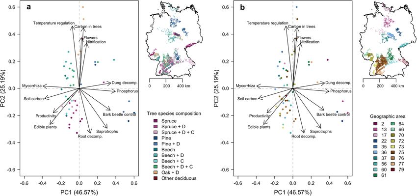
Simons et al. Forest Ecosystems    (2021) 8:5                                                                  Page 4 of 19

2013). We estimated the potential of our forests to har-        using the same elemental analyzer and total organic car-
bor edible fungi by analyzing fungal species pools in for-      bon was afterwards determined from the difference be-
est soils following the abovementioned description of           tween total and inorganic carbon (Schöning et al.
the joint soil-sampling campaign. Edible fungi were             2018a). Organic carbon stocks were determined by
identified following the criteria of the German Myco-           multiplying organic carbon concentrations with the total
logical Society, excluding those species with inconsistent      soil mass (0–10 cm) per unit area (< 2 mm) per m2 in
edible value (Deutsche Gesellschaft für Mykologie e.V.          each plot.
2015). We used species richness of edible fungi as a
proxy of potential edible fungi observation (See complete       Root decomposition
list in Felipe-Lucia et al. (2018) Supplementary Table 9).      Fine root decomposition plays an important role in
                                                                element cycling in forest ecosystems (Hobbie 1992). We
Potential nitrification activity                                measured decomposition of fine roots (< 2 mm) within
Nitrogen (N) can be a limiting element for plant growing        the upper 10 cm of the mineral soil. Three polyester lit-
and therefore limit the functioning of the ecosystem            terbags per plot, with a mesh size of 100 μm, were filled
(Vitousek and Howarth 1991; LeBauer and Treseder                with fine roots collected from 2-year-old European
2008). We investigated the nitrification process in forest      beech (Fagus sylvatica L.). These were buried in each of
soils in terms of potential nitrification activity. Soil sam-   the plots in October 2011 and were then harvested after
ples were collected during the joint soil-sampling cam-         12 months in October 2012. We used the percentage of
paign as described above. Potential nitrification measures      root litter mass loss as a proxy of decomposition (Solly
were derived from the abundance of nitrifying bacteria fol-     et al. 2011; Solly et al. 2014).
lowing (Hoffmann et al. 2007) and used as a proxy for po-
tential nitrification activity (Allan et al. 2015; Soliveres    Dung decomposition
et al. 2016). Two of the readings were excluded from the        Dung beetle communities contribute to the rapid de-
analysis because the standard deviation was three times         composition of fecal deposits from both wild mammals
larger than the mean and hence considered unexplained           and domestic livestock, representing a key ecosystem
outliers.                                                       service. We installed five dung piles (cow, sheep, horse,
                                                                wild boar, red deer) on each plot and collected the
Available phosphorus                                            remaining dung after 48 h. The average percentage of
Due to continuously high atmospheric N deposition,              dung dry mass removed (mostly by tunneling dung bee-
phosphorus (P) becomes increasingly important as a lim-         tles) was used as an indicator of dung removal rates
iting element for plant growth and therefore might limit        (Frank et al. 2017; Frank and Blüthgen 2018).
the functioning of the ecosystem (Holland et al. 2005;
Vitousek et al. 2010; Lang et al. 2017; Clausing et al.         Carbon storage in living trees
2020). We investigated the availability of P in forest soils    Trees are important carbon sinks as they store carbon in
by collecting soil samples as described above. Total P          their tissues via photosynthesis. In order to assess the
was extracted with 0.5 mol∙L− 1 NaHCO3 (pH = 8.5) fol-          amount of carbon stored in trees, we estimated the liv-
lowing the Olsen methodology (Olsen 1954; Alt et al.            ing tree volume on each plot as assessed in the second
2011; Sorkau et al. 2018) and measured using Inductively        forest inventory (2015–2016) (Kahl and Bauhus 2014;
Coupled Plasma/Optical Emission and Spectrometry                Schall and Ammer 2017). The living tree volume on
(ICP-OES, PerkinElmer Optima 5300 DV, S10 auto sam-             each plot which was converted to dry biomass using
pler). P concentrations in the extraction solution was          standard conversion factors of 0.46 for conifers (average
used as a proxy of P availability for plants (Felipe-Lucia      of spruce (0.43) and pine (0.49)) and 0.67 for broad-
et al. 2014).                                                   leaved trees (average of oak (0.66) and beech (0.68)), ac-
                                                                cording to Lohmann (2011). The carbon stored in a tree
Carbon stocks in the soil                                       is approximately 50% of its dry biomass (The Intergov-
Forest soils are important carbon pools. In order to esti-      ernmental Panel on Climate Change (IPCC) 2003).
mate the amount of carbon stored in forest topsoils, we
followed the abovementioned joint soil-sampling cam-            Bark beetle control
paign. An aliquot of < 2 mm sieved soil was homoge-             Natural bark beetle control is an important forest eco-
nized with a ball mill (RETSCH MM200, Retsch, Haan,             system service that can have an effect on other services
Germany) and used to determine total C concentrations           like production of quality timber and aesthetic value
by dry combustion in an elemental analyzer (VarioMax,           (Jactel et al. 2009; Bengtsson 2015). We assessed the
Hanau, Germany). Inorganic carbon was determined                abundance of potential pest species among the bark bee-
after combustion of organic carbon at 450 °C for 16 h           tles (i.e. ambrosia beetles), together with their
Simons et al. Forest Ecosystems (2021) 8:5 Page 5 of 19
antagonists. Ambrosia beetles cause substantial damage for forest productivity. We quantified productivity for
worldwide are thus considered as important pest species each of the 150 plots as mean annual increment (MAI)
(Grégoire et al. 2015). In Europe they impact broad- across rotation (i.e. culmination of MAI) for even-aged
leaved (e.g. Xyleborus dispar, Xylosandrus germanus, forests and as periodic annual increment (PAI) between
Trypodendron domesticum) as well as conifer trees (e.g. two forest inventories for uneven-aged and unmanaged
Trypodendron lineatum). Bark beetle control was forests (Schall and Ammer 2018a, 2018b). MAI was esti-
estimated from the ratio of bark beetle antagonists to mated based on site class or site maps of forest adminis-
bark beetles (i.e. tribe Xyleborini) based on collections of trations. Culmination of MAI is estimated on 70 to 100
bark beetles and their antagonists in pheromone traps years for Norway spruce (Picea abies), 70 to 90 years for
(Weisser and Gossner 2017). The collected specimen in- Scots pine (Pinus sylvestris), 120 to 140 years for oak
cluded species which attack broad-leaf trees as well as (Quercus spp.), and 140 to 160 years for European beech
species which attack conifer trees (Gossner et al. 2019). (Fagus sylvatica). PAI was estimated as the difference
Lineatin lures and ethanol were used as attractants for between the increment measured during the first forest
bark beetles and their antagonists. Traps were emptied inventory (2008–2011) and the second forest inventory
every second day during the main activity period of bark (2015–2016) of our plots divided by the time span in
beetles in 2010 (Gossner et al. 2019) and in weekly to years. All values are given as volume above bark (> 7 cm
monthly intervals afterwards. We standardized the data in diameter) in m3 per ha and year.
based on the method proposed by Grégoire et al. (2001).
We only considered bark beetles that are attracted by Edible vascular plants
lineatin and/or ethanol (i.e. species within the tribe Xyle- A common recreational use of forests is the collection of
borini) and predators and parasitoids that are mentioned fruits, nuts, berries and other plant parts for cooking
as antagonists of Xyleborini in the literature (Kenis et al. (Gamfeldt et al. 2013). We estimated the potential sup-
2004). Predator-prey ratios have been frequently used as ply of edible vascular plants based on two vegetation
measure of pest control potential in different systems surveys (in spring and summer to represent both flower-
(van der Werf et al. 1994; Klein et al. 2002; Bianchi et al. ing aspects) conducted in a 20 m × 20 m subplot in each
2013). Bark beetles vs. predators and parasitoids ratio of the plots in 2011 (Schäfer et al. 2017). Cover of each
was used as a proxy of bark beetle control. plant species was estimated across four different vegeta-
tion layers (herbs, shrubs < 5 m, trees 5–10 m, trees > 10
m), and the cumulative cover per vegetation layer was
Temperature regulation
used to calculate overall cover for each species. Wild
Forests buffer extreme temperatures due to their dense
edible plant species known to be collected were identi-
canopy cover (Frey et al. 2016). We collected data on air
fied by botanists from the Botanical Society of Bern
temperature 2 m above ground from climatic stations in-
(Bernische Botanische Gesellschaft) with knowledge on
stalled in each of the 150 plots. Records were quality
people preferences. Total cover of these species was used
controlled with respect to temporal dynamics and by
as a proxy of potential wild edible plants gathering (See
using data from neighboring stations. This results in
complete list in Felipe-Lucia et al. (2018) Supplementary
data for 143 plots suitable for the analysis (Hänsel and
Table 10).
Nauss 2019). Temperature regulation was defined as the
inverse of the diurnal temperature ranges (DTR) and
Culturally interesting vascular plants
calculated as the difference between daily maximum and
Plants blooming in early spring in forests are highly ap-
minimum temperature values (Scheitlin and Dixon
preciated for their aesthetic value (Bhattacharya et al.
2010). The inverse value of the average DTR per plot
2005). Other plant species are of special interest for in-
(1/DTR) was used as the proxy in order to facilitate the
terested non-experts and botanists, such as the forest
interpretation of the results, so higher values of the
specialists Helleborus spp., Asarum europaeum, Gallium
proxy mean higher temperature regulation of the forest
odoratum or Gagea lutea, Hepatica noblis and Anemone
plot (Felipe-Lucia et al. 2014). We used only 2011 as
nemorosa because of their unique flowering times or
most other indicators of ecosystem services were
their medicinal use (Schmidt et al. 2011; Lauber et al.
assessed in 2011.
2012). We estimated the potential aesthetic and educa-
tional value of forest plots following the abovementioned
Forest productivity methods description for edible vascular plants. Plant
Timber is one of the main products extracted from for- species of special interest for the general public or for
ests. Since accurate harvesting records were not available botanists were identified by botanists from the Botanical
for our calibration sites, we used the increment of the Society of Bern (Bernische Botanische Gesellschaft) with
stand in wood volume per hectare and year as a proxy knowledge on people preferences. Total cover of theseSimons et al. Forest Ecosystems (2021) 8:5 Page 6 of 19
species was used as a proxy of potential aesthetic value The stand density of all trees and of the main tree spe-
(complete list in Felipe-Lucia et al. (2018) Supplemen- cies is measured as the number of tree individuals per
tary Table 11). hectare which have a diameter at breast height (dbh) (at
1.3 m) larger than 7 cm. The following aggregated values
of the dbh were calculated: arithmetic mean, standard
Bird species richness
deviation, quadratic mean and arithmetic mean among
Forests provide good opportunities for birdwatching. In
the 50 largest trees. The standard deviation and coeffi-
order to estimate the bird-watching potential of forest
cient of variation were estimated based on the virtual
plots, we performed five bird surveys during breeding
angle-count method.
times (March to June 2011; Renner and Tschapka 2017)
Staudhammer and LeMay (2001) recommend the use
counting the number of individuals seen or heard during
of a tree size diversity index which is calculated as the
5 min at the center of each plot (Renner et al. 2014).
arithmetic mean of the Shannon diversity (H′) based on
The number of bird species was used as a proxy for bird
height classes (H′h) and the Shannon diversity based on
watching potential.
diameter classes (H′d). However, as information on tree
height was not available for 22 plots (mostly thickets
Forest structural and compositional parameters and abiotic with high tree densities), we only used the H′d based on
parameters classes of diameter at breast height (at 1.3 m) in steps of
We selected 18 forest parameters shown to affect ecosys- 4 cm (beginning with 7 cm). The basal area (m2) per hec-
tem functions and services that were available for both tare of all trees within a size class was used as the abun-
the calibration sites (Biodiversity Exploratories sites) and dance for the Shannon diversity. The diversity of
the predicted sites (German NFI plots). The parameters diameter classes was estimated based on the virtual
are related to stand structure (stand density, aggregated angle-count method. The number of tree species was
values of diameter at breast height, diversity of diameter counted based on trees from the virtual angle-count
classes, basal area of trees, relative crown cover) (Schall method. The overall crown projection area was calcu-
and Ammer 2017), tree species composition (number of lated by multiplying each tree’s crown projection area
tree species, relative cover of conifers, evenness of tree with its density per hectare. The relative crown projec-
species) (Schall and Ammer 2017), regeneration (num- tion area was calculated relative to 1 ha. The relative
ber and evenness of woody species and young trees, cover of conifers is based on the covered ground by all
relative cover of young Fagus sylvatica (L.) in the under- trees, which is calculated for a normalized reference area
storey) (Grassein and Fischer 2013), and deadwood (vol- (‘ideeller Flächenanteil’). Coniferous species in the Bio-
ume of coarse deadwood, diversity of deadwood types) diversity Exploratories mostly include spruce and pine.
(Kahl and Bauhus 2018). In the German National Forest Inventory, the following
All forest parameters were calculated on the calibra- coniferous species are listed: Norway spruce (Picea
tion sites based on a full inventory of all trees with a abies), Scots pine (Pinus sylvestris), Sitka spruce (Picea
diameter at breast height (dbh) larger than 7 cm within sitchensis), Douglas fir (Pseudotsuga menziesii), Larches
the 1-ha plots. In contrast, trees were assessed using (Larix spec.), Yew (Taxus baccata), other spruces (Picea
angle-count sampling or within circles of different size spec.), other pines (Pinus spec.), and other firs (Abies
depending on the height of the tree on the predicted spec.). The evenness of trees was calculated as Pielou’s
sites (Schmitz et al. 2008). Hence, not all trees within 1 evenness. This measure is the Shannon diversity (H′) di-
ha were assessed and measured for the predicted sites vided by the logarithm of species richness. The Shannon
and parameters had to be extrapolated to 1 ha from the diversity was calculated based on tree density as a substi-
individual tree counts. From each individual tree count, tute for abundance. Evenness of trees was calculated
the density per hectare of similar trees was calculated based on the full inventory as extrapolations based on
from the angle-counts. Extrapolation based on an aver- virtual angle-count measures were not biased (Supple-
age of four angle-counts gives very good estimations of mentary Fig. 1). The number of woody species in the
parameters of 1 ha, except for parameters which are shrub layer was assessed within a square of 400 m2 for
based on the diversity of trees in size and species iden- the Biodiversity Exploratories. In the German NFI, the
tity (Supplementary Fig. 1). For those parameters, the number of woody species in the shrub layer was based
sampling effect (higher diversity with more sampled in- on the species assessed in a 10-m circle for ground vege-
dividuals) leads to much higher values from the full in- tation assessment, which includes trees up to 4-m
ventory compared to the angle-count assessment. height. The evenness of woody species was calculated as
Hence, we used the average value of four simulated Pielou’s evenness with Shannon diversity based on the
angle-counts (instead of the full inventory) on the cali- percentage cover as a substitute for abundance. The
bration sites for forest parameters related to diversity. cover of young European beech trees within the shrubSimons et al. Forest Ecosystems (2021) 8:5 Page 7 of 19
layer was measured relative to the plot size, i.e. not rela- bund.de, downloaded 14th August 2017) with a grid size
tive to other species in the shrub layer. In the Biodiver- of 200 m from which the elevation above sea level was
sity Exploratories, the shrub layer was assessed within a extracted for the center of the plot. The aspect is given
square of 400 m2. In the German National Forest Inven- as the circular average over the plot area with 360°
tory, the shrub layer is assessed within a 10-m circle. equaling 0° as due north. The slope is given in percent.
Only individuals of Fagus sylvatica which are below 4 m For the Biodiversity Exploratories, aspect and slope were
in height were considered. Total volume of coarse dead- derived from a digital terrain model. Second-order finite
wood was estimated based on lying and standing dead- differences were used to derive slope and aspect, all
wood items with a diameter of at least 25 cm. Smaller values are means calculated over the entire plot area.
deadwood items and tree stumps were not considered. For the German National Forest Inventory, the inventory
The volume was calculated based on the length or plot coordinates were projected onto a digital terrain
height of each deadwood item and its diameter. The model of Germany (Geodatenzentrum, http://www.bkg.
German National Forest Inventory uses the assumption bund.de, downloaded 14th August 2017) with a grid size
that the deadwood item resembles a cylinder, thereby of 200 m from which the aspect and slope were
averaging between thinner or thicker parts of the dead- extracted for the center of the plot. The topsoil proper-
wood item (Schmitz et al. 2008): ties are described by the sand (2–0.063 mm), silt (0.063–
0.002 mm) and clay (< 0.002 mm) content in percent.
π ½diameter ðcmÞ2 length ðdmÞ For the Biodiversity Exploratories, topsoil properties
Volume m3 ¼
4 1002 10 were measured in the upper 10 cm of the mineral soil
As all deadwood items on the plot were assessed in the taken during a standardized joint soil-sampling cam-
Biodiversity Exploratories, the sum of all deadwood volumes paign in 2011. For the German National Forest Inven-
indicates the deadwood volume per hectare. As deadwood tory, the inventory plot coordinates were projected onto
items are only assessed within a circle of 5-m radius in the the map of topsoil physical properties for Europe based
German National Forest Inventory, the volume per hectare on LUCAS topsoil data108 with a grid size of 500 m. The
must be calculated with a correction factor: soil depth is measured in cm and describes the rooting
capacity of the soils. For the Biodiversity Exploratories,
3
m volume ðm3 Þ 1000 we determined soil depth by sampling a soil core in the
Volume ¼ with F korr
500 center of all plots in 2008. We used a motor-driven soil-
ha F korr
500
¼ 78:54 m 2 column cylinder with a diameter of 8.3 cm for the soil
sampling (Eijkelkamp, Giesbeek, The Netherlands). The
Diversity of deadwood was estimated as the Simpson combined thickness of all topsoil and subsoil horizons
diversity based on types of deadwood (standing, downed was used as a proxy of soil depth. For the German
tree, downed stem, other deadwood), the functional tree National Forest Inventory, the inventory plot coordinates
group (coniferous or deciduous) and decay stage (not were projected onto a map of soil depth (Bug 2015) for
decayed, beginning decay, proceeding decay and heavily Germany which is derived from profile data on the land
decomposed). In the German National Forest Inventory, use stratified soil map of Germany at scale 1:1,000,000.
40 unique combinations of categories were found, the The lower limit of a soil is bedrock, or a groundwater in-
Biodiversity Exploratories had 33 unique combinations fluenced horizon.
of categories. Each combination is treated as a species
and its overall volume is treated as abundance to calcu-
late the Simpson diversity. Selection of predictors and model development
All predictors showed normal distribution of resid-
Abiotic parameters uals. To reduce multi-collinearity among the initial
Abiotic variables included elevation above sea level, as- set of 18 forest structural and compositional parame-
pect and slope at the center of both the calibration and ters and 7 abiotic parameters, we applied a variance
the predicted sites (Nieschulze et al. 2018a; Nieschulze inflation analysis (Zuur et al. 2009) using the package
et al. 2018b). In addition, topsoil properties (sand, silt ‘fsmb’ (Nakazawa 2017) in R v.3.3.0 (R Core Team
and clay content) as well as soil depth were used (Schön- 2016), removing the predictor with the highest vari-
ing et al. 2018b). For the Biodiversity Exploratories, ele- ance inflation factor until all variance inflation factors
vation above sea level (m) was derived from a digital were below a threshold of 3 (Zuur et al. 2009). After
terrain model and taken at the center of the 1-ha plot. this procedure, 10 forest structural and compositional
For the German National Forest Inventory, the inventory parameters and 4 abiotic parameters remained as pre-
plot coordinates were projected onto a digital terrain dictors. Complete information on the final set of pre-
model of Germany (Geodatenzentrum, http://www.bkg. dictors was available for 124 of the 150 plots.Simons et al. Forest Ecosystems (2021) 8:5 Page 8 of 19 Our ecosystem service models were based on Gen- Definition of forest types for predictions eralized Linear Models. In order to ensure normal Each plot of the NFI should be considered as one of distribution of residuals, some indicators of ecosystem many sampling points, i.e. an individual inventory point services were transformed prior to model fitting: is not representative of the forest stand or forest type phosphorus availability, potential nitrification activity, around it. Hence, forest structural and compositional pa- bark beetle control, and cover of culturally interesting rameters have to be aggregated across several inventory plants were square-root-transformed; cover of edible points in order to accurately describe the characteristics plants was log-transformed. We applied model simpli- of a forest (Riedel et al. 2017). The set of inventory fication using the stepAIC function to find the most points over which parameters are aggregated are usually parsimonious model for each ecosystem service indi- defined as forest types which can be based on data de- cator. Models did not include any interactions be- rived from the inventory or based on additional informa- tween predictors as we wanted to derive purely tion. We defined forest types based on the large-scale additive models. We calculated a set of metrics for environmental characteristics of pre-defined geographic model quality: R2, RMSE (root mean squared error), areas (also termed growth areas) (vTI Agriculture and residual standard error of the whole model, and Forestry Research 2012), and refined those based on tree standard errors of estimated coefficients. Two of our species composition. The geographic areas were defined models (edible fungi richness and bird species rich- based on their geomorphological characteristics (i.e. bed- ness) showed low R2 values (less than 20% of ex- rock type and topography), climate and landscape his- plained variance) and were discarded from further tory (vTI Agriculture and Forestry Research 2012). Of analyses as key drivers of those ecosystem functions the 27,121 initial inventory plots, only 25,246 inventory were missing from our set of predictors. The other 13 plots could be associated with maps of abiotic informa- ecosystem service models had at least 30% of their tion (i.e. soil characteristics and topography), hence only variance explained and were retained. The additional those were used to define forest types. model quality metrics confirmed this selection (Sup- The German NFI covers both common and rare forest plementary Table 2). habitat types, but only three of the rare forest habitat While model quality metrics, like residual errors, are types are considered to be adequately represented: used to assess model quality for explanatory models Luzulo-Fagetum beech forests, Asperulo-Fagetum beech (i.e. models to understand mechanisms), estimation of forests and Galio-Carpinetum oak-hornbeam forests model quality for predictions requires a comparison of (Riedel et al. 2017). Hence, all forest inventory plots lo- observed and predicted values. We applied this by split- cated within other rare forest habitat types were ex- ting the Biodiversity Exploratories data into training cluded (23,304 plots remaining). We only included data and test data. The training data comprised a ran- geographic areas in which at least 40 inventory plots had dom subset of 70% of the plots, equally distributed been assessed (23,190 plots within 52 areas). Tree spe- across the three regions. The test dataset comprised the cies composition was defined based on the identity of remaining plots. For each ecosystem service indicator, the main tree species (Fagus sylvatica, Picea abies, Pinus models with the initial set of 25 predictors were calcu- sylvestris, Quercus spp. and others) and the functional lated using the stepwise selection procedure. The tree groups among the admixed tree species (pure stand, resulting coefficients were used to predict the potential only deciduous species, only coniferous species, decidu- supply of ecosystem services for the test plots. Average ous and coniferous species). Of the resulting 2652 pos- R2 values of 10-fold cross-validations from the function sible combinations of geographic areas and tree species ‘train’ in the R package ‘caret’ v6.0 were then used to composition, 1668 combinations were found among the assess the model’s predictive accuracy. The whole forest inventory plots and 148 combinations were repre- process was repeated 999 times with different sets of sented by at least 40 inventory plots (14,645 plots total). plots in the training and test dataset. For all ecosystem Of those 148 combinations, 115 included a tree species service indicators, the predictive accuracy of the models combination which was also found within the calibration was equal or higher than 30% and considered adequate sites (11,762 plots in total). Among those 115 combina- (Supplementary Table 2). However, the predicted tions, 53 were represented by at least 40 inventory plots values for edible fungi and bird species richness were with complete information on any predictor variable consistently higher than the observed values (Supple- (Supplementary Table 3). These 53 forest types cover mentary Fig. 2), so we excluded them from predictions 7003 inventory plots with complete information on at the national level. We provide the coefficients of forest and abiotic parameters (Supplementary Fig. 3). these ‘low quality’ models as a potential starting point Those plots were used to calculate average values and for the development of better models but advise against standard errors of all forest and abiotic parameters their direct use. per forest type.
Simons et al. Forest Ecosystems   (2021) 8:5                                                                     Page 9 of 19

Prediction of potential ecosystem service supply in            compare levels of potential ecosystem service supply for
Germany                                                        each forest type in relation to the other forest types, we
The average value and confidence intervals of each             calculated the relative level of potential ecosystem ser-
structural attribute were calculated from individual NFI       vice supply based on the maximum predicted level
plots and the upper and lower 95% confidence intervals         across forest types. For each forest type, we then
of all forest and abiotic parameters calculated for the 53     counted the number of ecosystem service indicators
forest types were compared to the observed ranges              which had a predicted relative level of 0.5, 0.75 and 0.9
within the calibration sites to check for outliers (Supple-    of the maximum predicted level. To assess the influence
mentary Fig. 4). The ranges of predictors across all forest    of variability in forest and abiotic parameters on the pre-
types fell within the observed range of the calibration        dicted level of potential ecosystem service supply per
sites except for soil depth for seven forest types. Hence,     forest types, we predicted the potential ecosystem service
we are confident that our extrapolations of the potential      supply for individual inventory plots and calculated aver-
supply of ecosystem services will not be confounded by         age and lower as well as upper confidence intervals for
exceeding the observed range of predictors. In addition,       each forest type. To assess which forest types showed
both sets of plots were compared with a principal com-         the highest level of multifunctionality, we counted the
ponent analysis (PCA) to check for distinct differences        number of ecosystem service indicators with at least
in multi-dimensional space (Supplementary Fig. 5). The         average levels of potential supply by a forest type. We
two datasets show considerable overlap in multi-               used the locations of the forest inventory points to assess
dimensional space, indicating that the Biodiversity Ex-        whether the current state of forests at the landscape-
ploratories cover a large proportion of forest structural      scale already fulfills the expectations of multi-purpose
combinations found among the 53 most dominant forest           forestry for Germany.
types in Germany. However, the inherent differences in
field assessments leads to a larger range of understorey       Results
diversity and evenness values within the Biodiversity Ex-      The ecosystem service models differed markedly be-
ploratories data compared to the forest inventory data         tween the ecosystem service indicators, both in terms of
(PC2 axis). On the other hand, the forest inventory plots      the predictors selected as important, and in terms of
show a larger range in tree species richness and tree size     their direction and strength of effects (Fig. 1 & Supple-
variability (PC3 axis). Overall, our results should be con-    mentary Table 2). For example, relative crown projection
sidered conservative because of the strict selection pro-      area had positive effects on carbon storage in trees and
cedure regarding forest types and number of inventory          temperature regulation, but negative effects on nitrifica-
plots included to ensure reliability of the predicted po-      tion potential and cover of edible plants. Proportion of
tential ecosystem service supply. While a broader defin-       silt in the soil, soil depth, relative conifer cover and vari-
ition of forest types will likely increase spatial coverage,   ability in tree diameter had a significant effect on the
it will also increase the variability in predictors within     majority of ecosystem service indicators. Relative cover
forest types and hence the uncertainty of predicted po-        of beech and evenness of woody species in the under-
tential ecosystem service supply.                              storey as well as diversity of deadwood types had signifi-
   Based on our ecosystem service models, we predicted         cant effects on one or two ecosystem service indicators.
the potential supply of ecosystem services for the 53 for-
est types. We used the R function ‘predict’ and back           Trade-offs and synergies
transformed those ecosystem service indicators which           The first PCA axis for potential ecosystem service supply
were normalized prior to modelling. For each forest            across 53 forest types in Germany explained 46.6% of
type, we calculated the potential supply of each ecosys-       the variability and revealed synergies between dung de-
tem service based on the average values of forest and          composition and phosphorus availability, and to a lesser
abiotic parameters across the inventory plots within each      extent with bark beetle control (Fig. 2). Those three eco-
forest type, resulting in 53 average levels of potential       system service indicators showed trade-offs with mycor-
ecosystem service supply. To identify groups of ecosys-        rhiza richness, soil carbon stocks and to a lesser extent
tem services delivered by the same forest type, i.e. syner-    with forest productivity and edible plants. The second
gies within forest types, we conducted a principal             axis (which explained 25.2% of the variability) revealed
component analysis (PCA) across the 53 forest types. To        strong synergies between temperature regulation, carbon
map the levels of potential ecosystem service supply, the      storage in trees, culturally interesting plants and nitrifi-
average values were assigned to the 7426 individual            cation potential. Forest types were clearly clustered in
German inventory plots which are located within the 53         the ordination depending on tree species composition,
forest types (including plots with incomplete informa-         with Norway spruce (Picea abies (L.) H. Karst) and Scots
tion on structural and compositional parameters). To           pine (Pinus sylvestris L.) separating forest types along
Simons et al. Forest Ecosystems         (2021) 8:5                                                                                            Page 10 of 19

 Fig. 1 Coefficients of ecosystem service models based on forest structural and compositional parameters and abiotic parameters. Points represent
 mean estimates, lines represent the 95% confidence intervals based on t-distributions (all variables were normally distributed). Non-significant (i.e. p >
 0.05) estimates are shown in grey, parameters without points were eliminated from the respective models through stepwise model simplification.
 Intercepts are shown separately from parameter coefficients for clarity; note the different ranges of the x-axes. Note that models for edible fungi and
 bird richness explain very little of the variability in the data (Supplementary Table 2) and were not used to predict potential ecosystem services supply

the first PC (principal component) axis, while broadleaf                        less important for differences in levels of potential eco-
forests and conifer forests separated along the second                          system service supply than tree species composition. Ex-
PC axis (Fig. 2a). Forests dominated by Norway spruce                           ceptions were the forest types from the northern and
were positively associated with root decomposition, ed-                         eastern lowland (areas 13 & 22), which formed a distinct
ible plants and saprotrophic fungal richness (cf. Awad                          cluster. Those areas are characterized by sandy soils,
et al. 2019), while forests dominated by European beech                         which only allow for low soil carbon stocks but achieve
(Fagus sylvatica L.) were positively associated with local                      high phosphorous availability (Grüneberg et al. 2013).
temperature regulation, culturally interesting plants (e.g.                     This particular soil texture also makes those areas suit-
Anemone nemorosa L.), carbon storage in trees and po-                           able for growing Scots pine, explaining the strong associ-
tential nitrification activity. The association between for-                    ation between pine-dominated forest types and
est types dominated by Norway spruce and edible plant                           phosphorus availability.
cover likely indicates high (historic) management inten-
sity, as many edible plants prefer the semi-open areas                          Level of potential ecosystem service supply
originating from management disturbances (e.g. Rubus                            Forest types did not only differ in terms of the main ecosys-
spec.) or the acidic soils usually found in conifer forests                     tem services they supported, they also differed greatly in the
(e.g. Vaccinium myrtillus L.). Forest types did not show                        level at which each service could be supplied (Fig. 3). For po-
clear clustering based on the geographic area (Fig. 2b),                        tential nitrification activity, phosphorus availability, bark bee-
indicating that large-scale environmental conditions                            tle control and cover of edible plants, most forest types
(geomorphology, climate and landscape history) were                             supplied only up to half of the level than the ‘best’ forest
Simons et al. Forest Ecosystems         (2021) 8:5                                                                                           Page 11 of 19

 Fig. 2 Trade-offs and synergies between ecosystem service indicators. Principal components analysis based on 13 ecosystem service indicators
 associated with tree species composition a and geographic area b and predicted for the 53 most dominant forest types in Germany. Spruce =
 Picea abies ((L.) H. Karst), Pine = Pinus sylvestris (L.), Beech = Fagus sylvatica (L.), Oak = Quercus spp., D= deciduous tree species, C = coniferous
 tree species

types did. For those services, a particular combination of tree                 services (root decomposition, potential nitrification
species composition and large-scale environmental condi-                        activity, mycorrhiza richness and carbon in living
tions (reflected by the geographic area) seems to be required                   trees). Central Germany showed high levels of regu-
to achieve high levels of potential supply. For some ecosys-                    lating services as well, but for a slightly different set
tem service indicators (e.g. potential nitrification activity or                of indicators (dung decomposition, phosphorus avail-
edible plants), different forest types from the same geo-                       ability, saprotrophic fungal richness and soil carbon
graphic area showed strong differences in the level at which                    stocks). Southern Germany showed highest levels of
each service was provided (Supplementary Fig. 3), indicating                    yet another set of regulating services (phosphorus
the importance of tree species composition. For other eco-                      availability, bark beetle control and temperature
system service indicators (e.g. decomposition, richness of                      regulation). Among those three regions, Southern
saprotrophs, carbon storage in trees and temperature regula-                    Germany showed a more heterogeneous pattern of
tion), differences in the predicted levels between forest types                 ecosystem services supply compared to Central or
were less pronounced (Fig. 3 & Supplementary Fig. 6).                           Northern Germany with all ecosystem service indica-
   No single forest type was superior to others in provid-                      tors showing average to high levels of supply at least
ing above-average levels of potential supply across all                         in some parts of Southern Germany (Fig. 5b). These
ecosystem service indicators (Fig. 4). Nevertheless, as                         patterns correspond to the geographic distribution of
each forest type achieved high levels for a subset of eco-                      the different forest types, with Southern Germany
system service indicators, some forest types are better                         showing a larger variety of forest types compared to
suited than others to provide a specific set of ecosystem                       the Center and North (Fig. 5a). Hence, multi-purpose
services at the stand scale.                                                    forest landscapes of a few hundred square-kilometers
                                                                                already exist in parts of Germany, and could be
Multifunctional forest areas                                                    achieved in other parts as well by increasing the mix
As the different forest types in this study represent a                         of tree species composition (under the constraints of
range of geographic areas, the differences among for-                           geographic area and environmental conditions).
est types translated into clear regional differences in
predicted levels of potential ecosystem service supply                          Discussion
(Fig. 5). Forest productivity levels (based on biomass                          No single forest type supplied all studied ecosystem ser-
increment) were highest in Northern Germany and                                 vices at high levels and the specific combination of
this region also showed highest levels of regulating                            which services could be supplied depended on the forest
Simons et al. Forest Ecosystems (2021) 8:5 Page 12 of 19 Fig. 3 Relative level of potential ecosystem service supply for each of the 53 most dominant forest types in Germany. Values are given relative to the maximum predicted level across forest types within each ecosystem service indicator. Colors indicate tree species composition and points are jittered horizontally to show the different geographic areas. Spruce = Picea abies ((L.) H. Karst), Pine = Pinus sylvestris (L.), Beech = Fagus sylvatica (L.), Oak = Quercus spp., D = deciduous tree species, C = coniferous tree species type. To achieve high levels of multifunctionality at the ecosystem services. Although tree species composition regional or landscape-level scale (i.e. a spatial scale that and site conditions are not independent, tree species includes numerous forest stands), multiple-purpose for- composition was more important in determining the po- estry needs to consider a mix of forest types, particularly tential supply of ecosystem services than large-scale en- of different tree species compositions in order to provide vironmental conditions. A change in forest type or tree a wide range of ecosystem services. species composition will likely not result in a loss of sup- The fact that each ecosystem service indicator is posi- ply for all ecosystem services. However, some ecosystem tively affected by a unique set of forest attributes and service indicators showed substantial variation within abiotic variables further indicates that multifunctionality forest types, highlighting that variability in forest attri- within forest types can only be achieved for subsets of butes and abiotic environment drives variability in levels
Simons et al. Forest Ecosystems         (2021) 8:5                                                                                           Page 13 of 19

 Fig. 4 Number of ecosystem service indicators which are supplied at or above a given threshold by each of the 53 dominant forest types in
 Germany. In total, 13 ecosystem services were modeled. Thresholds of relative ecosystem service supply were calculated relative to the maximum
 predicted level across all forest types within a service indicator. Colors indicate tree species composition and points are jittered horizontally to
 show the different geographic areas. Spruce = Picea abies ((L.) H. Karst, Pine = Pinus sylvestris (L.), Beech = Fagus sylvatica (L.), Oak = Quercus spp.,
 D = deciduous tree species, C = coniferous tree species

of potential supply. In addition, other factors not consid-                     chances that one or more forest types provide additional
ered here (both management-related and biotic or abi-                           ecosystem services, which could not be assessed or pre-
otic factors) likely also influence the potential supply of                     dicted in this study (e.g. scenic beauty, recreational value
ecosystem services. At the forest stand scale, guidelines                       or hunting). Such a large-scale approach needs to take
that aim to increase multifunctionality need to consider                        into account both the possibilities and limitations to es-
the existing trade-offs between ecosystem services, in                          tablishing a particular forest type in a region, as well as
order to set realistic goals. This is especially true for for-                  the spatial variability of demands for ecosystem services
est types aiming at timber production, as productivity                          (Burkhard et al. 2012). Hence, achieving multifunctional
showed synergies only with a small number of ecosystem                          forest landscapes which supply ecosystem services where
services. Nevertheless, multifunctionality within forest                        they are needed, and which consider both managers and
types can possibly be improved via changes to those for-                        users of ecosystem services, requires long-term and
est structural attributes that have strong effects on the                       spatially explicit planning of forest management over
potential supply of particular ecosystem services.                              large areas. The diversity of forest ownership within a
  High levels of multifunctionality can also be achieved                        given area complicates such top-down planning ap-
at the landscape scale by promoting those forest types                          proaches but may in turn already provide multifunc-
that provide complementary subsets of ecosystem ser-                            tional forest landscapes where differently managed forest
vices. Within such an optimized landscape, each forest                          stands provide different ecosystem services.
type would provide high levels of a subset of the desired
ecosystem services at the stand level, theoretically result-                    Conclusions
ing in high levels of all ecosystem services at the land-                       Both the assessment and the management of ecosystem
scape scale. A mix of forest types will also increase the                       services require a consistent mapping of forest structural
You can also read