MVS2D: Efficient Multi-view Stereo via Attention-Driven 2D Convolutions
←
→
Page content transcription
If your browser does not render page correctly, please read the page content below

MVS2D: Efficient Multi-view Stereo via Attention-Driven 2D Convolutions

                                                                 Zhenpei Yang1,∗ Zhile Ren2 Qi Shan2                            Qixing Huang1
                                                                        1                                                       2
                                                                          The University of Texas at Austin                       Apple

                                                                     Abstract
arXiv:2104.13325v2 [cs.CV] 11 Dec 2021

                                             Deep learning has made significant impacts on multi-
                                         view stereo systems. State-of-the-art approaches typically
                                         involve building a cost volume, followed by multiple 3D
                                         convolution operations to recover the input image’s pixel-
                                         wise depth. While such end-to-end learning of plane-
                                         sweeping stereo advances public benchmarks’ accuracy,
                                         they are typically very slow to compute. We present MVS2D,
                                         a highly efficient multi-view stereo algorithm that seam-
                                         lessly integrates multi-view constraints into single-view net-
                                         works via an attention mechanism. Since MVS2D only
                                         builds on 2D convolutions, it is at least 2× faster than all
                                         the notable counterparts. Moreover, our algorithm pro-                      Figure 1. Inference frame per second (FPS) vs. depth error (Ab-
                                         duces precise depth estimations and 3D reconstructions,                     sRel) on ScanNet [7]. Our model achieve significant reduction in
                                         achieving state-of-the-art results on challenging bench-                    inference time, while maintaining state-of-the-art accuracy.
                                         marks ScanNet, SUN3D, RGBD, and the classical DTU
                                         dataset. our algorithm also out-performs all other algo-
                                         rithms in the setting of inexact camera poses. Our code is                  ever, these approaches work best for rectified stereo pairs,
                                         released at https://github.com/zhenpeiyang/                                 and extending them to multi-view is nontrivial. 2) Con-
                                         MVS2D                                                                       structing a differential 3D cost volume [12,14,15,28,51,52].
                                                                                                                     These algorithms significantly improve the accuracy of
                                                                                                                     MVS, but at the cost of heavy computational burdens. Fur-
                                         1. Introduction                                                             thermore, the predicted depth map by 3D convolution usu-
                                                                                                                     ally contains salient artifacts which have to be rectified by a
                                             Multi-view Stereo (MVS) aims to reconstruct the under-                  2D refinement network [15]. 3) Maintain a global scene rep-
                                         lying 3D scene or estimate the dense depth map using mul-                   resentation and fuse multi-view information through ray-
                                         tiple neighboring views. It plays a key role in a variety of                casting features from 2D images [27]. This paradigm can-
                                         3D vision tasks. With high-quality cameras becoming more                    not handle large-scale scenes because of the vast memory
                                         and more accessible, there are growing interests in develop-                consumption on maintaining a global representation.
                                         ing reliable and efficient stereo algorithms in various appli-                 Aside from multi-view depth estimation, we have also
                                         cations, such as 3D reconstruction, augmented reality, and                  witnessed the tremendous growth of single-view depth pre-
                                         autonomous driving. As a fundamental problem in com-                        diction networks [21, 30, 46, 50, 54]. As shown in Table
                                         puter vision, MVS has been extensively studied [9]. Recent                  3, Bts [21] has achieved impressive result on ScanNet [7].
                                         research shows that deep neural networks, especially con-                   Single-view depth prediction roots in learning feature repre-
                                         volutional neural networks (CNNs), lead to more accurate                    sentations to capture image semantics, which is orthogonal
                                         and robust systems than traditional solutions. Several ap-                  to correspondence-computation in multi-view techniques.
                                         proaches [20, 55] report exceptional accuracy on challeng-                  A natural question is how to combine single-view depth
                                         ing benchmarks like ScanNet [7] and SUN3D [45].                             cues and multi-view depth cues.
                                             State-of-the-art CNN-based multi-view approaches typi-
                                                                                                                        We introduce MVS2D that combines the strength of
                                         cally fall into three categories: 1) Variants of a standard 2D
                                                                                                                     single-view and multi-view depth estimations. The core
                                         UNet architecture with feature correlation [22, 26]. How-
                                                                                                                     contribution is an attention mechanism that aggregates fea-
                                             ∗ Experiments are conducted by Z. Yang at The University of Texas       tures along epipolar lines of each query pixel on the refer-
                                         at Austin. Email: yzp@utexas.edu                                            ence images. This module captures rich signals from the

                                                                                                                 1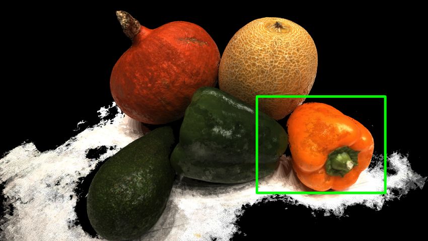
reference images. Most importantly, it can be easily inte-          ficiency of regular tensor operations. [15, 51] proposed an
grated into standard CNN architectures defined on the input         end-to-end plane-sweeping stereo approach that constructs
image, introducing relatively low computational cost.               learnable 3D cost volume. While MVSNet [51] focuses on
    Our attention mechanism possesses two appealing char-           the reconstruction of 3D scene, DPSNet [15] focuses on
acteristics: 1) Our network only contains 2D convolutions.          evaluating the per-view depth-map accuracy. Researchers
2) Besides relying on the expressive power of 2D CNNs,              have also explored other 3D representations to regularized
the network seamlessly integrates single-view feature rep-          the prediction, such as point clouds [4], surface normals
resentations and multi-view feature representations. Conse-         [20], or meshes [44]. There are also several benchmark
quently, MVS2D is the most efficient approach compared to           datasets for this task [1, 7, 34, 40, 45, 53].
state-of-the-art algorithms (See Figure 1). It is 48× faster        Cost volume for multi-view stereo. A recent line of
than NAS [20], 39× faster than DPSNet [15], 10× faster              works on multi-view stereo utilizes the notion of cost vol-
than MVSNet [51], 4.7× faster than FastMVSNet [55], and             ume, which contains feature matching costs for a pair of
almost 2× speed-up over the most recent fastest approach            images [13]. This feature representation has been suc-
PatchmatchNet [42]. In the mean-time, MVS2D achieves                cessfully implemented in various pixel-wise matching tasks
state-of-the-art accuracy.                                          like optical flow [35]. Authors of MVSNet [51] and DP-
    Intuitively, the benefit of MVS2D comes from the early          SNet [15] proposed to first construct a differentiable cost
fusion of the intermediate feature representations. The out-        volume and then use the power of 3D CNNs to regularize
come is that the intermediate feature representations con-          the cost volume before predicting per-pixel depth or dispar-
tain rich 3D signals. Furthermore, MVS2D offers ample               ity. Most recent state-of-the-art approaches follow such a
space where we can design locations of the attention mod-           paradigm [4,12,23,28,52,55]. However, the size of the cost
ules to address different inputs. One example is when the           volume (C×K×H ×W ) is linearly related to the number of
input camera poses are inaccurate, and corresponding pix-           depth hypotheses K. These approaches are typically slow
els deviate from the epipolar lines on the input reference          in both training and inference. For example, DPSNet [15]
images. We demonstrate a simple solution, which installs            takes several days to train on ScanNet; NAS [20] takes
multi-scale attention modules on an encoder-decoder net-            even longer because of its extra training of a depth-normal
work. In this configuration, corresponding pixels in down-          consistency module. Recently, Murez et al. [27] proposed
sampled reference images lie closer to the epipolar lines,          to construct a volumetric scene representation from a cali-
and MVS2D detect and rectify correspondences automati-              brated image sequence for scene reconstruction. However,
cally.                                                              their approach is very memory demanding due to the high
    We conduct extensive experiments on challenging                 memory requirement of global volumetric representations.
benchmarks ScanNet [7], SUN3D [45], RGBD [34] and                   Efficient multi-view stereo. Several recent works aim at
Scenes11 [34]. MVS2D achieves the state-of-the-art per-             reducing the cost of constructing cost volumes. Duggal et
formance on nearly all the metrics. Qualitatively, compared         al. [8] prune the disparity search range during cost volume
to recent approaches [15,20,51,55], MVS2D helps generate            construction. Xu et al. [47] integrate adaptive sampling
higher quality 3D reconstruction outputs.                           and deformable convolution into correlation-based meth-
                                                                    ods [22, 26] to achieve efficient aggregation. Several other
2. Related Works                                                    works [12, 36, 52] employ iterative refinement procedures.
                                                                    The above approaches either only work for pairwise recti-
Recent advances of multi-view stereo. Multi-view stereo             fied stereo matching tasks or have to construct a 3D cost-
algorithms can be categorized into depth map-based ap-              volume. Alternatively, Poms et al. [29] learn how to merge
proaches, where the output is a per-view depth map, or              patch features for 3D reconstruction efficiently. Badki et
point-based approaches, where the output is a sparse re-            al. [2] convert depth estimation as a classification task, but
construction of the underlying scene (cf. [9]). Many tra-           the resulting accuracy is not state-of-the-art. Recently, Yu et
ditional multi-view stereo algorithms follow a match-then-          al. [55] proposed constructing a sparse cost-volume through
reconstruct paradigm [10] that leverages the sparse-nature          regular sub-sampling and then applying Gauss-Newton iter-
of feature correspondences. Such a paradigm typically fails         ations to refine the dense depth map. Wang et al. [42] pro-
to reconstruct textureless regions where correspondences            posed a highly-efficient Patchmatch-inspired approach for
are not well-defined. Along this line, Zbontar et al. [56]          MVS tasks. In contrast, we take an orthogonal approach
provided one of the first attempts to bring the power of fea-       based on the attention-driven 2D convolutions.
ture learning into multi-view stereo. They proposed a super-        Attention in 3D vision Attention mechanism has shown
vised feature learning approach to find the correspondences.        prominent results on both natural language processing
Recently, researchers have found that depth map-based ap-           (NLP) tasks [41] and vision tasks [43]. Recently, self-local
proaches [14, 15, 17, 51, 52] are more favorable than those         attention [31, 33] has shown promising results compared
that follow the match-and-reconstruct paradigm. A key ad-           with the convolution-based counterparts. Several recent
vantage of these approaches is that they can utilize the ef-        works that build an attention mechanism in MVS [23, 25,

                                                                2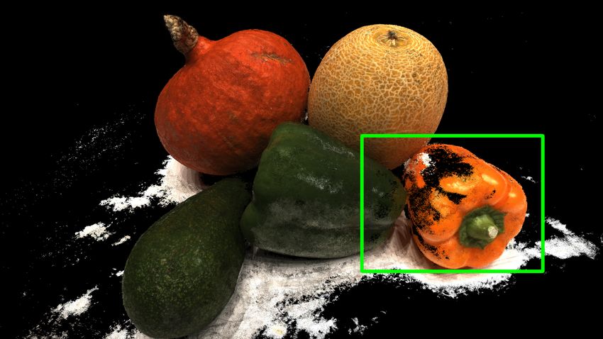
Figure 2. Network architecture of MVS2D. We employ a 2D UNet structure F to make the depth prediction on I0 , while injecting multi-
view cues extracted using G through the Epipolar Attention Module. Dashed arrows only exist in Ours-robust model (Section 3.4). We
highlight that the proposed epipolar attention module can be easily integrated into most 2D CNNs.

57], but still rely on 3D CNNs and cannot avoid construct-           depth d0 ∈ R of p0 , the unprojected 3D point of p0 is
ing a heavy-weighted cost volume. A promising direction
                                                                                       p0 (d0 ) = d0 · (K−1 p0 ).
is to utilize a geometry-aware 2D attention mechanism. Re-
cent works have shown that this paradigm works well for                 Similarly, we use pi (d0 ) and pi (d0 ) to denote respec-
active sensing [5, 39] and neural rendering [37]. Motivated          tively the 3D coordinates and homogeneous coordinates of
by these works, we propose an epipolar attention module in           p0 (d0 ) in the i-th image’s coordinate system. They satisfy
this paper. The key contribution is a network design that ag-
gregates single-view depth cues and multi-view depth cues                              pi (d0 ) = Ri p0 (d0 ) + ti ,
to output accurate MVS outputs.                                                        pi (d0 ) = Kpi (d0 ).                    (1)
                                                                     3.2. Network Design Overview
3. Approach                                                             In this paper, we innovate developing a multi-view stereo
                                                                     approach that only requires 2D convolutions. Specifi-
    We provide an overview of the network architecture of
                                                                     cally, similar to most single-view depth prediction net-
MVS2D in Fig. 2. We operate in a multi-view stereo setting
                                                                     works, our approach progressively computes multi-scale ac-
(Sec. 3.1), and employ a 2D UNet structure in our network
                                                                     tivation maps of the source image and outputs a single depth
design (Sec. 3.2). Our core contribution is the epipolar at-
                                                                     map. The difference is that certain intermediate activation
tention module (Sec. 3.3–3.4), which is highly accurate and
                                                                     maps combine both the output of a 2D convolution opera-
efficient (Sec. 3.5) for depth estimation (Sec. 3.6).
                                                                     tor applied to the previous activation map and the output of
                                                                     an attention module that aggregates multi-view depth cues.
3.1. Problem Setup                                                   This attention module, which is the main contribution of
                                                                     this paper, matches each pixel of the source image and cor-
    We aim to estimate the per-pixel depth for a source im-          responding pixels on epipolar lines on the reference images.
age I0 ∈ Rh×w×3 , given n reference images {Ii }ni=1 of              The matching procedure utilizes learned feature activations
the same size captured at nearby views. We assume the                on both the source image and the reference images. The out-
source image and the reference images share the same in-             put is encoded using learned depth codes compatible with
trinsic camera matrix K ∈ R3×3 , which is given. We also             the activation maps of the source image.
assume we have a good approximation of the relative cam-                Formally speaking, our goal is to learn a feed-forward
era pose between the source image and each reference im-             network F with L layers. With Fj ∈ Rhj ×wj ×mj we
age Ti = (Ri |ti ) ,where Ri ∈ SO(3) and ti ∈ R3 . Ti                denote the output of the j-th layer, where mj is its fea-
usually comes from the output of a multi-view structure-             ture dimension, hj and wj are its height and width. Note
from-motion algorithm. Our goal is to recover the dense              that the first layer F1 ∈ Rh1 ×w1 ×3 denotes the input,
pixel-wise depth map associated with I0 .                            while the last layer FL ∈ RhL ×wL denotes the out-
    We denote the homogeneous coordinate of a pixel p0 in            put layer containing depth prediction. Between two con-
                                            T
the source image I0 as p0 = p0,1 , p0,2 , 1 . Given the              secutive layers are a general convolution operator Cj :

                                                                 3
Rhj ×wj ×mj → Rhj ×wj ×mj+1 (it can incorporate stan-                    inside and outside samples, respectively. Define
dard operators such as down-sampling, up-sampling, and
                                                                                        v jin    0 ≤ pki,1 < w, 0 ≤ pki,2 < h, pki,3 ≥ 0,

max-pooling) and an optional attention module Aj :
                                                                          v jik =
Rhj ×wj ×mj → Rhj ×wj ×mj :                                                             v jout                 otherwise
                                                                                                                                              (4)
                     Fj+1 = Cj ◦ Aj ◦ Fj .                               where pki = (pki,1 , pki,2 , 1)T , pki = (pki,1 , pki,2 , pki,3 )T . To
                                                                         enhance the expressive power of Gj , we further include a
As we will see immediately, the attention operator Aj uti-               trainable linear map A1j that depends only on feature of p0
lizes features extracted from the reference images. Without              and not on the matching results. Combing with (3) and (4),
these attention operations, F becomes a standard encoder-                we define
decoder network for single-view depth prediction.
                                                                                                                      n X
                                                                                                                        K
   Another characteristic of this network design is that the                                                   wj     X
                                                                         Aep           n        1
                                                                                                           N ( √ ik )(v jik ck ))
                                                                          j (p0 , {Ii }i=1 ) = Aj (Gj (p0 ))+
convolution operator Cj implicitly aggregates multi-view                                                        mj
                                                                                                   i=1 k=1
depth cues extracted at adjacent pixels. This approach pro-                                                                (5)
motes consistent correspondences among adjacent pixels                   where N is the softmax normalizing function over
that share the same epipolar line or have adjacent epipolar              wj
lines.                                                                   √ ik , 1
                                                                          mj     ≤ k ≤ K. Substituting (5) into (2), the final at-
                                                                         tention module is given by
3.3. Epipolar Attention Module
                                                                                    Aj (p0 ) = A0j (Fj (p0 )) + A1j (Gj (p0 ))
   We proceed to define Aj (p0 ), which is the action of Aj                                          n X
                                                                                                       K
on each pixel p0 . It consists of two parts:                                                         X             wj
                                                                                                 +             N ( √ ik )(v jik   ck )).
                                                                                                     i=1 k=1
                                                                                                                    mj
        Aj (p0 ) =   Aep           n
                      j (p0 , {Ii }i=1 )   + A0j (Fj (p0 )).   (2)
                                                                            Note that the attention modules at different layers have
As we will define next, Aep                n
                              j (p0 , {Ii }i=1 ) uses trainable          different weights. Eq. 3 can be viewed as a similarity score
depth codes to encode the matching result between p0 and                 between source pixel and correspondence candidates. In
the reference images. A0j : Rmj → Rmj is composed of                     Fig. 3, we visualize the learned attention scores for query
an identity map and a trainable linear map that transforms               pixels. The true corresponding pixels on reference images
the feature associated with p0 in Fj .                                   have larger learned weights along epipolar lines.
   The formulation of Aep               n
                           j (p0 , {Ii }i=1 ) uses the epipolar
context of p0 . It consists of samples on the epipolar lines
of p0 on the reference images. These samples are obtained
from sampling the depth values d0 of p0 and then applying
(1). With pki we denote the k-th sample on the i-th reference
image.
   To match p0 and pki , we introduce a feature extraction
network G that has identical architecture (except the atten-
tion modules) as Fjmax where jmax is the maximum depth
of any attention module of F. With Gj (I0 , p0 ) ∈ Rmj and
Gj (Ii , pki ) ∈ Rmj we denote the extracted features of p0
and pki , respectively. Following the practice of scaled-dot
product attention [41], we introduce two additional train-
able linear maps f j0 : Rmj → Rmj and f jref : Rmj →
Rmj to transform the extracted features. With this setup,                Figure 3. Visualization of attention scores. Left: source view with
we define the matching score between p0 and pki as                       query pixels. Right: reference view with candidate pixels, where
                                                                         opacity is learned attention scores.
        j                        T j
           = f j0 (Gj (I0 , p0 ))  f ref (Gj (Ii , pki )) .

       wik                                                     (3)
                                                                         3.4. Attention Design for Robust Multi-View Stereo
     It remains to 1) model samples that are occluded in the
                                                j
reference images, and 2) bridge the weights wik   defined in                Since the attention module assumes that the correspond-
(3) and the input to the convolution operator Cj . To this               ing pixels lie on the epipolar lines, the accuracy of MVS2D
end, we first introduce trainable mask codes cjk ∈ Rmj                   depends on the relative poses’ accuracy between the refer-
that correspond to the k-th depth sample. We then introduce              ence images and the source image. When input poses are
v jin ∈ Rmj and v jout ∈ Rmj , which are trainable codes for             accurate, our experiments suggest a single attention module

                                                                     4
Method FPS (3)↑ FPS(7)↑ FPS(11) ↑ Param (M) ↓ AbsRel↓ 4. Experimental Results
Bts [21] 17.0 - - 46.8 0.117
MVSNet [51] 4.1 2.4 1.6 1.1 0.094
DPSNet [15] 1.1 0.7 0.5 4.2 0.094 4.1. Datasets
FastMVS [55] 9.0 6.0 4.3 0.4 0.089
PatchmatchNet [42] 21.8 11.6 8.5 0.2 0.133 ScanNet [7] The ScanNet dataset contains 807 unique
NAS [20] 0.9 0.6 0.4 18.0 0.086
Ours-mono 94.7 - - 12.3 0.145
scenes with image sequences captured from different cam-
Ours-robust 17.5 10.1 7.1 24.4 0.059 era trajectories. We sample 86324 triple images (one source
Ours 42.9 29.1 21.8 13.0 0.059 image and two reference images) for training and 666 triple
images for testing. Our setup ensures the scene correspond-
Table 1. Quantitative comparison on computational efficiency.
ing to test images is not included in the training set.
FPS (V ) only applies to multi-view methods [15, 20, 51, 55] and
means we use V images to make the prediction. Note that num- DeMoN [40] We further validate our method on DeMoN,
bers under the AbsRel metric are identical to those in Table 3 for which is a dataset introduced by [40] for multi-view depth
ease of comparison. We use a single Nvidia V100 GPU for mea- estimation. The training set consists of three data sources,
suring FPS. Please refer to section 4.4 for additional discussions. SUN3D [45], RGBD [34], and Scenes11 [40]. SUN3D and
RGBD contain real indoor scenes, while Scenes11 is syn-
thetic. In total, there are 79577 training pairs for SUN3D,
at the second layer of F is sufficient. This leads to a highly 16786 for RGBD, and 71820 for Scenes11.
efficient multi-view stereo network. DTU [1] While our approach is designed for multi-view
When the input poses are inexact, we address this issue depth estimation, we additionally validate our method on
by installing attention modules at different resolutions of the DTU dataset, which has been considered as one of the
the input images, i.e., at different layers of F. This ap- main test-bed for multi-view reconstruction algorithms.
proach ensures that the corresponding pixels lie sufficiently 4.2. Evaluation Metrics
close to the epipolar lines at those resolutions at coarse res-
olutions. Since the convolution operations Cj at different Efficiency. We benchmark our methods against baseline
layers of F aggregate multi-view features extracted at dif- methods on the frame per second (FPS) during inference.
ferent pixels, we find this simple network design implicitly We additionally compare the FPS when increasing the num-
rectifies inexact epipolar lines. Figure 2 illustrates the at- ber of reference views.
tention modules under these two cases. Depth Accuracy. We use the conventional metrics of depth
estimation [21] (See Table 2). Note that in contrast to
monocular depth estimation evaluation, we do not factor out
3.5. Computational Complexity the depth scale before evaluation. The ability to correctly
predict scale will render our method more applicable.
For the sake of simplicity in notation, we assume the fea-
Scene Reconstruction Quality. We further apply MVS2D
ture channel dimension C is the same in both input and out-
for scene reconstruction. We follow PatchmatchNet [42] to
put. We denote the feature height and width as H and W
fuse the per-view depth map into a consistent 3D model.
respectively and denote the kernel size of convolution layers
Please refer to supp. material for quantitative and more
as k. Suppose there are K depth samples, the complexity of
qualitative comparisons.
3D convolution is O(C 2 HW Kk 3 ).
Robustness under Noisy Input Pose. We perturb the input
For our approach, the computational complexity for ex- relative poses Tj during training and report the model per-
ecuting one layer of C ◦ A is in total O(CHW (Ck 2 + K)). formance on ScanNet test set in Table 8. Please refer to the
Since K is usually less than Ck 2 , our module leads to a Kk supp. material for details of the pose perturbing procedures.
times reduction in computation. The actual runtime can be
found in Table 1. 1 |di −d∗
P i|
q
1
P
− d∗i )2
AbsRel N d∗
ii
RMSE N i (di
P (di −d∗i )2 q
1 1
− log d∗i )2
P
SqRel d∗ RMSELog i (log di
qN i i N
1 1 ∗
d∗i |
P P
3.6. Training Details AbsDiff N i |di − Log10 N i | log10 di − log10 di |
∗
k 1
P di di k 1
P ∗
δ < 1.25 N i (max( d∗
i
, di ) < 1.25 ) thre@x N i I(|di − di | < x)
Our implementation is based on Pytorch. For ScanNet
and DeMoN, we simply optimize the L1 loss between pre- Table 2. Quantitative metrics for depth estimation. di is the pre-
dicted and ground truth depth. For DTU, we introduce a dicted depth; d∗i is the ground truth depth; N corresponds to all
pixels with the ground-truth label. I is the indicator function.
simple modification, as was done in [18], to simultaneously
train a confidence prediction. We use Adam [19] optimizer
with = 10−8 , β = (0.9, 0.999). We use a starting learn- 4.3. Baseline Approaches
ing rate 2e−4 for ScanNet, 8e−4 for DeMoN and 2e−4 for
DTU. Please refer to supp. material for more training de- MVSNet [51] is an end-to-end plane sweeping stereo ap-
tails. proach based on 3D-cost volume.
5
Method                       AbsRel ↓   SqRel ↓     log10 ↓    RMSE ↓     RMSELog ↓      δ < 1.25 ↑    δ < 1.252 ↑   δ < 1.253 ↑
              Bts [21]                 0.117      0.052       0.049      0.270       0.151          0.862          0.966         0.992
             Bts∗ [21]                 0.088      0.035       0.038      0.228       0.128          0.916          0.980         0.994
         MVSNet [51]                   0.094      0.042       0.040      0.251       0.135          0.897          0.975         0.993
         FastMVS [55]                  0.089      0.038       0.038      0.231       0.128          0.912          0.978         0.993
          DPSNet [15]                  0.094      0.041       0.043      0.258       0.141          0.883          0.970         0.992
             NAS [20]                  0.086      0.032       0.038      0.224       0.122          0.917          0.984         0.996
    PatchmatchNet [42]                 0.133      0.075       0.055      0.320       0.175          0.834          0.955         0.987
            Ours-mono                  0.145      0.065       0.061      0.300       0.173          0.807          0.957         0.990
          Ours-mono∗                   0.103      0.037       0.044      0.237       0.135          0.892          0.984         0.996
           Ours-robust                 0.059      0.016       0.026      0.159       0.083          0.965          0.996         0.999
                 Ours                  0.059      0.017       0.026      0.162       0.084          0.963          0.995         0.999
Table 3. Depth evaluation results on ScanNet [7]. We compare against both multi-view depth estimation methods [15, 20, 42, 51, 55]
and a state-of-the-art single-view method [21]. Our approach achieve significant improvements over top-performing method NAS [20] on
AbsRel. The improvements are consistent across all metrics.

                        Method        AbsRel ↓   AbsDiff ↓    SqRel ↓   RMSE ↓      RMSELog ↓      δ < 1.25 ↑   δ < 1.252 ↑   δ < 1.253 ↑
                     COLMAP [32]       0.623      1.327        3.236     2.316        0.661          0.327         0.554         0.718
    SUN3D (Real)

                       DeMoN [40]      0.214      2.148        1.120     2.421        0.206          0.733         0.922         0.963
                     DeepMVS [14]      0.282      0.604        0.435     0.944        0.363          0.562         0.739         0.895
                     DPSNet-U [15]     0.147      0.336        0.117     0.449        0.196          0.781         0.926         0.973
                         NAS [20]      0.127      0.288        0.085     0.378        0.170          0.830         0.944         0.978
                        Ours-robust    0.100      0.231        0.057     0.313        0.140          0.895         0.966         0.991
                              Ours     0.099      0.224        0.055     0.304        0.137          0.893         0.970         0.993
                     COLMAP [32]       0.539      0.940        1.761     1.505        0.715          0.275         0.500         0.724
    RGBD (Real)

                       DeMoN [40]      0.157      1.353        0.524     1.780        0.202          0.801         0.906         0.962
                     DeepMVS [14]      0.294      0.621        0.430     0.869        0.351          0.549         0.805         0.922
                     DPSNet-U [15]     0.151      0.531        0.251     0.695        0.242          0.804         0.895         0.927
                         NAS [20]      0.131      0.474        0.213     0.619        0.209          0.857         0.929         0.945
                        Ours-robust    0.078      0.311        0.156     0.443        0.146          0.926         0.945         0.954
                              Ours     0.082      0.325        0.165     0.440        0.147          0.921         0.939         0.948
                     COLMAP [32]       0.625      2.241        3.715     3.658        0.868          0.390         0.567         0.672
    Scenes11 (Syn)

                       DeMoN [40]      0.556      1.988        3.402     2.603        0.391          0.496         0.726         0.826
                     DeepMVS [14]      0.210      0.597        0.373     0.891        0.270          0.688         0.894         0.969
                       DPSNet [15]     0.050      0.152        0.111     0.466        0.116          0.961         0.982         0.988
                         NAS [20]      0.038      0.113        0.067     0.371        0.095          0.975         0.990         0.995
                        Ours-robust    0.041      0.141        0.066     0.410        0.099          0.979         0.991         0.994
                              Ours     0.046      0.155        0.080     0.439        0.107          0.976         0.989         0.993
Table 4. Depth evaluation results on SUN3D, RGBD, and Scenes11 datasets(synthetic). The numbers for COLMAP, DeMoN, DeepMVS,
DPSNet, and NAS are obtained from [20]. We achieve significant improvements on SUN3D and RGBD. We show the best number in bold
and the second best with underline.

DPSNet [15] shares similar spirit of MVSNet [51] but focus                       Similar to Bts∗ , we also report the results factoring out the
on accurate depth map prediction.                                                global scale for Ours-mono∗ .
NAS [20] is a recent work that jointly predicts consistent                       Ours-robust is our method with multi-scale epipolar atten-
depth and normal, using extra normal supervision.                                tion module applied on F.
FastMVSNet [55] is a recent variant to MVSNet which ac-                          Ours is our method with epipolar attention module applied
celerate the computation by computing sparse cost volume.                        only in F’s second layer.
Bts [21] is a state-of-the-art single view depth prediction
network. It incorporates planar priors into network design.                      4.4. Result Analysis
Additionally, we use an asterisk sign ‘∗’ to denote an oracle                    Comparison on Efficiency. We compare against both
version Bts∗ , where we use the ground truth depth map to                        single-view methods [21] and multi-view methods [15, 20,
factor out the global scale.                                                     51, 55]. The inference speed of our method is comparable
PatchmatchNet [42] is one of the most recent state-of-the-                       to single-view methods [21] and significantly outperforms
art efficient MVS algorithm.                                                     other multi-view methods [15, 20, 51, 55]. Evaluations are
Ours-mono is our method without the epipolar attention                           done on ScanNet [7]. Our method is 48× faster than NAS,
module, thus equivalent to single-view depth estimation.                         39× faster than DPSNet, 10× faster than MVSNet, and 4×

                                                                           6
Bts [21]          FastMVSNet [55]           NAS [20]            PatchmatchNet [42]     MVS2D (Ours)               G.T.

Figure 4. Qualitative results on depth prediction. Each row corresponds to one test example. The region without ground truth depth labels
is colored white in GT. Our prediction outperforms both the single-view depth estimation method [21] and other multi-view methods.
   PatchmatchNet
   PatchmatchNet                                CasMVSNet
                                                CasMVSNet                                   MVS2D
                                                                                            MVS2D (ours)
                                                                                                  (ours)

 Figure 5. Qualitative 3D reconstruction results on DTU dataset. MVS2D produces more complete reconstruction in texture-less region.

faster than the FastMVSNet. Please refer to the supp. for               simply infer the global scaling factor from multi-view cues.
more details.                                                           Compared with the single-view model, our model only in-
Comparison on Depth Estimation. MVS2D achieves con-                     curs a 5.8% increase in parameters. Such efficiency will
siderable improvements in the depth prediction accuracy                 enable multi-view methods to embrace a much larger 2D
(see Table 3). On ScanNet, our approach outperforms                     convolutional network which is not possible before.
MVSNet by large margins, reducing AbsRel error from                        On other datasets, MVS2D also performs favorably (see
0.094 to 0.059. The improvements are consistent across                  Table 4). We achieve the AbsRel error of 0.078 on the
most other metrics. Remarkably, our approach also outper-               RGBD dataset, while the next best NAS only achieves
forms NAS, which uses more parameters and runs 48 times                 0.131. Although MVS2D excels at adapting to the scene
slower. We visualize some depth predictions in Figure 4.                prior, it is encouraging that it also performs well on the
   Our approach yields significant improvements over                    Scenes11 dataset, a synthetic scene with randomly placed
single-view baselines. Adding multi-view cues improves                  objects. We ranked second on the Scenes11 dataset on Ab-
the AbsRel of ours-mono from 0.145 to 0.059 on ScanNet.                 sRel. Please refer to the supp. material for experiments on
Since single-view has scale-ambiguity, we further investi-              our generalization ability to novel datasets.
gate whether our methods will still be favorable when fac-              Evaluations on DTU. We evaluate on DTU dataset follow-
toring out the scale. The results show that when eliminat-              ing the practice of [42]. We use 4 reference views and 96
ing the scale, ours-mono∗ has AbsRel 0.103, which is still a            depth samples uniformly placed in the inverse depth space
                                                                            1      1
significant improvement. This means our approach does not               ([ 935. , 425. ]). The quantitative results can be found in Table

                                                                   7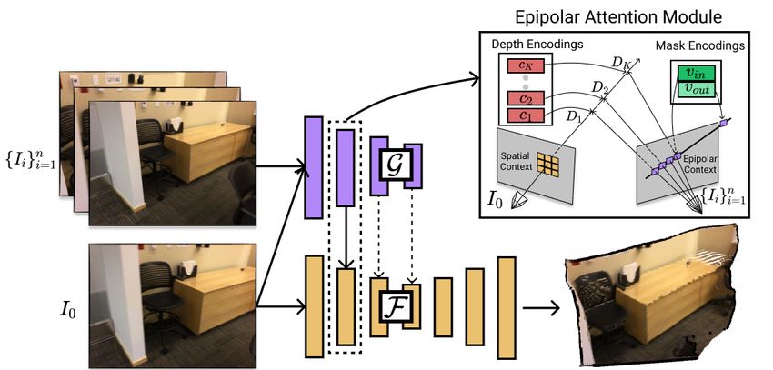
Methods           Acc.(mm)       Comp.(mm)         Overall(mm)       computations (as shown in Table 1).
        Camp [3]           0.835           0.554              0.695
        Furu [10]          0.613           0.941              0.777
        Tola [38]          0.342           1.190              0.766
                                                                                    Metric       MVSNet     DPSNet    Ours     Ours-robust
      Gipuma [11]          0.283           0.873              0.578                AbsRel ↓       0.094      0.094    0.059      0.059
    SurfaceNet [16]        0.450           1.040              0.745              AbsRel (p) ↓     0.113      0.126    0.073      0.070
     MVSNet [51]           0.396           0.527              0.462                  ∆↓           0.019      0.032    0.014      0.011
    R-MVSNet [52]          0.383           0.452              0.417               δ < 1.25 ↑      0.897      0.871    0.983      0.965
      CIDER [48]           0.417           0.437              0.427             δ < 1.25 (p) ↑    0.851      0.807    0.947      0.952
    P-MVSNet [24]          0.406           0.434              0.420                  ∆↓           0.046      0.064    0.016      0.013
   Point-MVSNet [4]        0.342           0.411              0.376
   Fast-MVSNet [55]        0.336           0.403              0.370
   CasMVSNet [12]          0.325           0.385              0.355          Table 8. Different methods’ performance under noisy input poses
      UCS-Net [6]          0.338           0.349              0.344          on ScanNet [7]. We notice that most methods suffer from signif-
  CVP-MVSNet [49]          0.296           0.406              0.351          icant performance drops. Our method with multi-scale epipolar
  PatchMatchNet [42]       0.427           0.277              0.352          aggregation shows notable robustness.
    MVS2D (Ours)           0.394           0.290              0.342
Table 5. Quantitative results on the evaluation set of DTU [1]. We           Ablation Study on Depth Encoding. The ablation study
bold the best number and underline the second best number.                   of our depth code design can be found in Table 9. We tested
                                                                             four code types. ‘Uniform’ serves as a sanity check, where
      Metric      FPS640 × 480 ↑   FPS1280 × 640 ↑   FPS1536 × 1152 ↑        we use the same code vector for all depth hypotheses. In
  PatchmatchNet        16.5             6.30               4.57
  MVS2D (Ours)         36.4             10.9               7.3               other words, the network does not extract useful informa-
                                                                             tion from the reference images. ‘Linear’ improves on uni-
Table 6. Speed benchmark on DTU dataset. We show FPS (frame
per second) on three input resolutions. We use one source image              form encoding by scaling a base code vector with the cor-
and 4 reference images.                                                      responding depth value. ‘Cosine’ codes are identical to the
                                                                             one used in [41]. ‘Learned‘ codes are optimized end-to-end.
      Metric       RMSE(mm)↓       thre@0.2↑   thre@0.5↑    thre@1.0↑        We can see that learning the codes end-to-end leads to no-
  PatchmatchNet      32.348           0.169       0.387        0.610
  MVS2D (Ours)       14.769           0.238       0.504        0.718         ticeable performance gains. One explanation is that these
                                                                             learned codes can adapt to the single-view feature represen-
Table 7. Depth evaluation on DTU validation set. We show the
                                                                             tations of the source image.
root mean square error and the percentage of errors fall below
0.2/0.5/1.0mm thresholds.
                                                                                  Metric         Uniform   Linear     Cosine     Learned
5. MVS2D is the best on overall score and the second-best                        AbsRel ↓         0.139    0.128      0.064       0.059
completeness score. Such performance is encouraging since                       δ < 1.25 ↑        0.815    0.840      0.961       0.964
our method is quite simple: it is just a single-stage proce-                     RMSE ↓           0.293    0.283      0.166       0.156
dure without using any multi-stage refinement as commonly
used in recent MVS algorithms ( [12, 42, 52]). We show                       Table 9. Ablation study on different depth encodings. We can see
some qualitative results of 3D reconstruction on DTU ob-                     that jointly training depth encodings gives the best performance.
jects in Figure 5. Qualitatively, our reconstruction is typi-
cally more complete on flat surface areas. The behavior is
reasonable because our approach utilizes strong single-view
                                                                             5. Conclusions and Limitations
priors. We also compare the inference speed with the recent                  Conclusions. We proposed a simple yet effective method
SOTA PatchmatchNet [42]. Our approach yield around 2x                        for multi-view stereo. The core of our method is to inte-
speed up as shown in Table 6. Lastly, as our method was                      grate single-view and multi-view cues during the prediction
mainly designed for multi-view depth estimation, we addi-                    jointly. Such a design not only improves the performance
tionally examine the depth evaluation metrics. Since DTU                     but also has the appealing factor of being efficient. Fur-
does not have ground truth depth for the test set, we report                 thermore, we have demonstrated the trade-off between in-
the depth evaluation results on the validation set. As ex-                   put pose accuracy and network complexity. When the input
pected, MVS2D is better than PatchmatchNet in terms of                       pose is exact, we can leverage minimum additional com-
depth metrics, and the performance gap there is wider than                   putation to inject more multi-view information through the
in 3D Reconstruction. The results can be found in Table 7.                   epipolar attention.
Comparison on Robustness under Noisy Pose. As shown                          Limitations. One limitation of our approach is that the
in Table 3, Ours-robust (multi-scale cues) and Ours (single-                 network is trained in a way that adapted to data distribu-
scale cues) perform similarly when the input poses are ac-                   tion well, which might makes it less generalizable to out-
curate. However, as shown in Table 8, multi-scale aggrega-                   of-distribution testing data. In the future, we propose to
tion is preferred when the input poses are noisy. It suggests                address this issue by developing robust training losses. An-
that when having inaccurate training data, it is necessary to                other limitation is that the proposed attention mechanism
incorporate multi-scale cues, though at a cost of increased                  does not explicitly model the consistency between different

                                                                         8
pixels on the same epipolar line. We plan to address this is- [13] Asmaa Hosni, Christoph Rhemann, Michael Bleyer, Carsten
sue by developing novel attention mechanisms to explicitly Rother, and Margrit Gelautz. Fast cost-volume filtering
enforce those constraints. for visual correspondence and beyond. IEEE Transac-
tions on Pattern Analysis and Machine Intelligence (TPAMI),
35(2):504–511, 2012. 2
References
[14] Po-Han Huang, Kevin Matzen, Johannes Kopf, Narendra
[1] Henrik Aanæs, Rasmus Ramsbøl Jensen, George Vogiatzis, Ahuja, and Jia-Bin Huang. DeepMVS: Learning multi-view
Engin Tola, and Anders Bjorholm Dahl. Large-scale data for stereopsis. In Proceedings of the IEEE Conference on Com-
multiple-view stereopsis. International Journal of Computer puter Vision and Pattern Recognition (CVPR), pages 2821–
Vision (IJCV), 120(2):153–168, 2016. 2, 5, 8 2830, 2018. 1, 2, 6
[2] Abhishek Badki, Alejandro Troccoli, Kihwan Kim, Jan [15] Sunghoon Im, Hae-Gon Jeon, Stephen Lin, and In So
Kautz, Pradeep Sen, and Orazio Gallo. Bi3D: Stereo depth Kweon. DPSNet: End-to-end deep plane sweep stereo. In In-
estimation via binary classifications. In Proceedings of the ternational Conference on Learning Representations (ICLR),
IEEE Conference on Computer Vision and Pattern Recogni- 2019. 1, 2, 5, 6
tion (CVPR), pages 1600–1608, 2020. 2 [16] Mengqi Ji, Juergen Gall, Haitian Zheng, Yebin Liu, and Lu
[3] Neill DF Campbell, George Vogiatzis, Carlos Hernández, Fang. Surfacenet: An end-to-end 3d neural network for mul-
and Roberto Cipolla. Using multiple hypotheses to improve tiview stereopsis. In Proceedings of the IEEE International
depth-maps for multi-view stereo. In Proceedings of the Eu- Conference on Computer Vision (ICCV), pages 2307–2315,
ropean Conference on Computer Vision (ECCV), pages 766– 2017. 8
779. Springer, 2008. 8 [17] Abhishek Kar, Christian Häne, and Jitendra Malik. Learn-
[4] Rui Chen, Songfang Han, Jing Xu, and Hao Su. Point-based ing a multi-view stereo machine. In Advances in Neural
multi-view stereo network. In Proceedings of the IEEE In- Information Processing Systems (NeurIPS), pages 364–375,
ternational Conference on Computer Vision (ICCV), pages 2017. 2
1538–1547, 2019. 2, 8 [18] Alex Kendall and Yarin Gal. What uncertainties do we need
[5] Ricson Cheng, Ziyan Wang, and Katerina Fragkiadaki. in bayesian deep learning for computer vision? Advances in
Geometry-aware recurrent neural networks for active visual Neural Information Processing Systems (NeurIPS), 2017. 5
recognition. In Advances in Neural Information Processing [19] Diederik P. Kingma and Jimmy Ba. Adam: A method for
Systems (NeurIPS), pages 5086–5096, 2018. 3 stochastic optimization. In Yoshua Bengio and Yann LeCun,
[6] Shuo Cheng, Zexiang Xu, Shilin Zhu, Zhuwen Li, Li Erran editors, International Conference on Learning Representa-
Li, Ravi Ramamoorthi, and Hao Su. Deep stereo using adap- tions (ICLR), 2015. 5
tive thin volume representation with uncertainty awareness. [20] Uday Kusupati, Shuo Cheng, Rui Chen, and Hao Su. Nor-
In Proceedings of the IEEE Conference on Computer Vision mal assisted stereo depth estimation. Proceedings of the
and Pattern Recognition (CVPR), pages 2524–2534, 2020. 8 IEEE Conference on Computer Vision and Pattern Recog-
[7] Angela Dai, Angel X. Chang, Manolis Savva, Maciej Hal- nition (CVPR), 2020. 1, 2, 5, 6, 7
ber, Thomas Funkhouser, and Matthias Nießner. ScanNet: [21] Jin Han Lee, Myung-Kyu Han, Dong Wook Ko, and
Richly-annotated 3D reconstructions of indoor scenes. In Il Hong Suh. From big to small: Multi-scale local planar
Proceedings of the IEEE Conference on Computer Vision guidance for monocular depth estimation. arXiv preprint
and Pattern Recognition (CVPR), 2017. 1, 2, 5, 6, 8 arXiv:1907.10326, 2019. 1, 5, 6, 7
[8] Shivam Duggal, Shenlong Wang, Wei-Chiu Ma, Rui Hu, [22] Zhengfa Liang, Yiliu Feng, Yulan Guo, Hengzhu Liu, Wei
and Raquel Urtasun. DeepPruner: Learning efficient stereo Chen, Linbo Qiao, Li Zhou, and Jianfeng Zhang. Learning
matching via differentiable patchmatch. In Proceedings for disparity estimation through feature constancy. In Pro-
of the IEEE International Conference on Computer Vision ceedings of the IEEE Conference on Computer Vision and
(ICCV), pages 4384–4393, 2019. 2 Pattern Recognition (CVPR), pages 2811–2820, 2018. 1, 2
[9] Yasutaka Furukawa and Carlos Hernández. Multi-view [23] Xiaoxiao Long, Lingjie Liu, Wei Li, Christian Theobalt, and
stereo: A tutorial. Found. Trends. Comput. Graph. Vis., 9(1- Wenping Wang. Multi-view depth estimation using epipo-
2):1–148, June 2015. 1, 2 lar spatio-temporal networks. In Proceedings of the IEEE
[10] Yasutaka Furukawa and Jean Ponce. Accurate, dense, and Conference on Computer Vision and Pattern Recognition
robust multiview stereopsis. IEEE Transactions on Pattern (CVPR), 2021. 2
Analysis and Machine Intelligence (TPAMI), 32(8):1362– [24] Keyang Luo, Tao Guan, Lili Ju, Haipeng Huang, and Yawei
1376, 2009. 2, 8 Luo. P-MVSNet: Learning patch-wise matching confidence
[11] Silvano Galliani, Katrin Lasinger, and Konrad Schindler. aggregation for multi-view stereo. In Proceedings of the
Massively parallel multiview stereopsis by surface normal IEEE International Conference on Computer Vision (ICCV),
diffusion. In Proceedings of the IEEE International Confer- pages 10452–10461, 2019. 8
ence on Computer Vision (ICCV), pages 873–881, 2015. 8 [25] Keyang Luo, Tao Guan, Lili Ju, Yuesong Wang, Zhuo Chen,
[12] Xiaodong Gu, Zhiwen Fan, Siyu Zhu, Zuozhuo Dai, Feitong and Yawei Luo. Attention-aware multi-view stereo. In Pro-
Tan, and Ping Tan. Cascade cost volume for high-resolution ceedings of the IEEE Conference on Computer Vision and
multi-view stereo and stereo matching. In Proceedings of the Pattern Recognition (CVPR), pages 1590–1599, 2020. 2
IEEE Conference on Computer Vision and Pattern Recogni- [26] Nikolaus Mayer, Eddy Ilg, Philip Hausser, Philipp Fischer,
tion (CVPR), pages 2495–2504, 2020. 1, 2, 8 Daniel Cremers, Alexey Dosovitskiy, and Thomas Brox. A
9large dataset to train convolutional networks for disparity, recurrent networks. In Proceedings of the IEEE Conference
optical flow, and scene flow estimation. In Proceedings of the on Computer Vision and Pattern Recognition (CVPR), pages
IEEE Conference on Computer Vision and Pattern Recogni- 2595–2603, 2019. 3
tion (CVPR), pages 4040–4048, 2016. 1, 2 [40] Benjamin Ummenhofer, Huizhong Zhou, Jonas Uhrig, Niko-
[27] Zak Murez, Tarrence van As, James Bartolozzi, Ayan Sinha, laus Mayer, Eddy Ilg, Alexey Dosovitskiy, and Thomas
Vijay Badrinarayanan, and Andrew Rabinovich. Atlas: End- Brox. Demon: Depth and motion network for learning
to-end 3D scene reconstruction from posed images. In Pro- monocular stereo. In Proceedings of the IEEE Conference
ceedings of the European Conference on Computer Vision on Computer Vision and Pattern Recognition (CVPR), pages
(ECCV), 2020. 1, 2 5622–5631, 2017. 2, 5, 6
[28] Guang-Yu Nie, Ming-Ming Cheng, Yun Liu, Zhengfa Liang, [41] Ashish Vaswani, Noam Shazeer, Niki Parmar, Jakob Uszko-
Deng-Ping Fan, Yue Liu, and Yongtian Wang. Multi-level reit, Llion Jones, Aidan N Gomez, Lukasz Kaiser, and Illia
context ultra-aggregation for stereo matching. In Proceed- Polosukhin. Attention is all you need. Advances in Neural
ings of the IEEE Conference on Computer Vision and Pattern Information Processing Systems (NeurIPS), 2017. 2, 4, 8
Recognition (CVPR), pages 3283–3291, 2019. 1, 2 [42] Fangjinhua Wang, Silvano Galliani, Christoph Vogel, Pablo
[29] Alex Poms, Chenglei Wu, Shoou-I Yu, and Yaser Sheikh. Speciale, and Marc Pollefeys. Patchmatchnet: Learned
Learning patch reconstructability for accelerating multi-view multi-view patchmatch stereo. In Proceedings of the IEEE
stereo. In Proceedings of the IEEE Conference on Computer Conference on Computer Vision and Pattern Recognition
Vision and Pattern Recognition (CVPR), pages 3041–3050, (CVPR), pages 14194–14203, 2021. 2, 5, 6, 7, 8
2018. 2 [43] Xiaolong Wang, Ross Girshick, Abhinav Gupta, and Kaim-
[30] Xiaojuan Qi, Renjie Liao, Zhengzhe Liu, Raquel Urtasun, ing He. Non-local neural networks. In Proceedings of the
and Jiaya Jia. Geonet: Geometric neural network for joint IEEE Conference on Computer Vision and Pattern Recogni-
depth and surface normal estimation. In Proceedings of the tion (CVPR), pages 7794–7803, 2018. 2
IEEE Conference on Computer Vision and Pattern Recogni- [44] Yuesong Wang, Tao Guan, Zhuo Chen, Yawei Luo, Keyang
tion (CVPR), pages 283–291, 2018. 1 Luo, and Lili Ju. Mesh-guided multi-view stereo with pyra-
[31] Prajit Ramachandran, Niki Parmar, Ashish Vaswani, Irwan mid architecture. In Proceedings of the IEEE Conference
Bello, Anselm Levskaya, and Jonathon Shlens. Stand-alone on Computer Vision and Pattern Recognition (CVPR), pages
self-attention in vision models. Advances in Neural Informa- 2039–2048, 2020. 2
tion Processing Systems (NeurIPS), 2019. 2 [45] Jianxiong Xiao, Andrew Owens, and Antonio Torralba.
[32] Johannes L. Schönberger and Jan-Michael Frahm. Structure- SUN3D: A database of big spaces reconstructed using sfm
from-motion revisited. In Proceedings of the IEEE Confer- and object labels. In Proceedings of the IEEE International
ence on Computer Vision and Pattern Recognition (CVPR), Conference on Computer Vision (ICCV), pages 1625–1632,
pages 4104–4113, 2016. 6 2013. 1, 2, 5
[33] Peter Shaw, Jakob Uszkoreit, and Ashish Vaswani. Self- [46] Dan Xu, Elisa Ricci, Wanli Ouyang, Xiaogang Wang, and
attention with relative position representations. In Proceed- Nicu Sebe. Multi-scale continuous CRFs as sequential deep
ings of the 2018 Conference of the North American Chap- networks for monocular depth estimation. In Proceedings
ter of the Association for Computational Linguistics: Hu- of the IEEE Conference on Computer Vision and Pattern
man Language Technologies, Volume 2 (Short Papers), pages Recognition (CVPR), 2017. 1
464–468, 2018. 2 [47] Haofei Xu and Juyong Zhang. AANet: Adaptive aggregation
[34] J. Sturm, N. Engelhard, F. Endres, W. Burgard, and D. Cre- network for efficient stereo matching. In Proceedings of the
mers. A benchmark for the evaluation of RGB-D SLAM sys- IEEE Conference on Computer Vision and Pattern Recogni-
tems. In IEEE/RSJ International Conference on Intelligent tion (CVPR), pages 1959–1968, 2020. 2
Robots and Systems (IROS), 2012. 2, 5 [48] Qingshan Xu and Wenbing Tao. Learning inverse depth re-
[35] Deqing Sun, Xiaodong Yang, Ming-Yu Liu, and Jan Kautz. gression for multi-view stereo with correlation cost volume.
PWC-Net: CNNs for optical flow using pyramid, warping, In AAAI Conference on Artificial Intelligence (AAAI), pages
and cost volume. In Proceedings of the IEEE Conference 12508–12515, 2020. 8
on Computer Vision and Pattern Recognition (CVPR), pages [49] Jiayu Yang, Wei Mao, Jose M Alvarez, and Miaomiao Liu.
8934–8943, 2018. 2 Cost volume pyramid based depth inference for multi-view
[36] Vladimir Tankovich, Christian Häne, Sean Fanello, Yinda stereo. In Proceedings of the IEEE Conference on Computer
Zhang, Shahram Izadi, and Sofien Bouaziz. HITNet: Hier- Vision and Pattern Recognition (CVPR), pages 4877–4886,
archical iterative tile refinement network for real-time stereo 2020. 8
matching. arXiv preprint arXiv:2007.12140, 2020. 2 [50] Zhenpei Yang, Li Erran Li, and Qixing Huang. Strumononet:
[37] Josh Tobin, OpenAI Robotics, and Pieter Abbeel. Geometry- Structure-aware monocular 3d prediction. In Proceedings
aware neural rendering. Advances in Neural Information of the IEEE Conference on Computer Vision and Pattern
Processing Systems (NeurIPS), 2019. 3 Recognition (CVPR), 2021. 1
[38] Engin Tola, Christoph Strecha, and Pascal Fua. Efficient [51] Yao Yao, Zixin Luo, Shiwei Li, Tian Fang, and Long Quan.
large-scale multi-view stereo for ultra high-resolution im- Mvsnet: Depth inference for unstructured multi-view stereo.
age sets. Machine Vision and Applications, 23(5):903–920, In Proceedings of the European Conference on Computer Vi-
2012. 8 sion (ECCV), pages 767–783, 2018. 1, 2, 5, 6, 8
[39] Hsiao-Yu Fish Tung, Ricson Cheng, and Katerina Fragki- [52] Yao Yao, Zixin Luo, Shiwei Li, Tianwei Shen, Tian Fang,
adaki. Learning spatial common sense with geometry-aware and Long Quan. Recurrent MVSNet for high-resolution
10multi-view stereo depth inference. In Proceedings of the
IEEE Conference on Computer Vision and Pattern Recog-
nition (CVPR), pages 5525–5534, 2019. 1, 2, 8
[53] Yao Yao, Zixin Luo, Shiwei Li, Jingyang Zhang, Yufan
Ren, Lei Zhou, Tian Fang, and Long Quan. Blendedmvs:
A large-scale dataset for generalized multi-view stereo net-
works. Proceedings of the IEEE Conference on Computer
Vision and Pattern Recognition (CVPR), 2020. 2
[54] Wei Yin, Yifan Liu, Chunhua Shen, and Youliang Yan. En-
forcing geometric constraints of virtual normal for depth pre-
diction. In Proceedings of the IEEE International Confer-
ence on Computer Vision (ICCV), pages 5684–5693, 2019.
1
[55] Zehao Yu and Shenghua Gao. Fast-MVSNet: Sparse-to-
dense multi-view stereo with learned propagation and gauss-
newton refinement. In Proceedings of the IEEE Conference
on Computer Vision and Pattern Recognition (CVPR), pages
1949–1958, 2020. 1, 2, 5, 6, 7, 8
[56] Jure Zbontar and Yann LeCun. Computing the stereo match-
ing cost with a convolutional neural network. In Proceed-
ings of the IEEE Conference on Computer Vision and Pattern
Recognition (CVPR), pages 1592–1599, 2015. 2
[57] Xudong Zhang, Yutao Hu, Haochen Wang, Xianbin Cao, and
Baochang Zhang. Long-range attention network for multi-
view stereo. In IEEE Winter Conference on Applications of
Computer Vision (WACV), pages 3782–3791, 2021. 2
11You can also read