Modeling the effects of socioeconomic development and climate change on the microbial water quality in the catchment of Lake Mälaren

Modeling the effects of
socioeconomic development and
climate change on the microbial
water quality in the catchment of
Lake Mälaren
Master’s thesis in Infrastructure and Environmental Engineering

Erik Söderlund
Mathias Lennartsson

DEPARTMENT OF ARCHITECTURE AND CIVIL ENGINEERING
DIVISION OF WATER ENVIRONMENT TECHNOLOGY

CHALMERS UNIVERSITY OF TECHNOLOGY
Gothenburg, Sweden 2021
www.chalmers.se

MASTER’S THESIS ACEX30

Modeling the effects of socioeconomic development and climate change on the microbial water
 quality in the catchment of Lake Mälaren
 Master’s Thesis in the Master’s Programme Infrastructure and Environmental Engineering
 Erik Söderlund
 Mathias Lennartsson

 Department of Architecture and Civil Engineering
 Division of Water Environment Technology
 CHALMERS UNIVERSITY OF TECHNOLOGY
 Göteborg, Sweden 2021

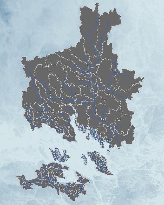
Modeling the effects of socioeconomic development and climate change on the microbial water
quality in the catchment of Lake Mälaren

Master’s Thesis in the Master’s Programme Infrastructure and Environmental Engineering
Erik Söderlund
Mathias Lennartsson

©ERIK SÖDERLUND, MATHIAS LENNARTSSON, 2021

Examensarbete ACEX30
Institutionen för arkitektur och samhällsbyggnadsteknik
Chalmers tekniska högskola, 2021

Department of Architecture and Civil Engineering
Division of Water Environment Technology
Chalmers University of Technology
SE-412 96 Göteborg
Sweden
Telephone: + 46 (0)31-772 1000

Cover:
Modeled catchment area surrounding Lake Mälaren.

Modeling the effects of socioeconomic development and climate change on the microbial water
quality in the catchment of Lake Mälaren

Master’s Thesis in the Master’s Programme Infrastructure and Environmental Engineering
Erik Söderlund
Mathias Lennartsson

Department of Architecture and Civil Engineering
Division of Water Environment Technology
Chalmers University of Technology

Abstract
Surrounding catchment areas can influence drinking water suppliers negatively. The anthropogenic
activities from the catchment areas contribute with fecal contamination to surface water. These activities
are expected to change in the future due to socioeconomic development but also due to climate change,
which alters hydrological parameters. To assess the effect of future changes on microbial concentrations
related to hydrological processes, a useful method could be to use Shared Socioeconomic Pathways
(SSP) together with Representative Concentration Pathways (RCP) and a hydrological modeling
programme such as ArcSWAT, which other recent studies have begun to use.

In this report, the potential impact of socioeconomic and climate changes on the microbial water quality
in the catchment of Lake Mälaren was investigated. This was done by identifying fecal contamination
sources, setting up a baseline scenario, and developing and including future scenarios. The baseline
scenario was simulated in ArcSWAT for the period 2010-2020, and the future scenarios were simulated
for two time periods, 2040-2050 and 2090-2100.

The performance of the model with respect to water flow in three selected subbasins ranged from fair
to good and was overall acceptable. The simulated concentrations of E. coli and Cryptosporidium in the
outlet of Stäket were in general high in contrast to the observed or modeled concentrations in previous
studies. The concentrations in two other subbasins had a greater similarity with the observed or modeled
concentrations in previous studies. According to the model, the most critical contributors to E. coli
concentrations were wastewater treatment plants and on-site wastewater treatment systems, while for
Cryptosporidium it was wastewater treatment plants and agriculture. Wastewater treatment plants
contributed to the majority of the E. coli and Cryptosporidium concentrations when present in a water
course. According to the modeling results, a scenario with high level of adaptations (improved
wastewater treatment, buffer zones and reduced water use) would generally reduce the E. coli and
Cryptosporidium concentrations, while a scenario with lower level of adaptations would generally have
similar E. coli and Cryptosporidium concentrations compared to the baseline scenario. Scenarios with
climate change alone would also generally have similar E. coli and Cryptosporidium concentrations
compared to the baseline scenario.

 I

Contents
1. Introduction .................................................................................................................................................. 1
 1.1 Aim and objectives .............................................................................................................................. 2
 1.2 Limitations ............................................................................................................................................. 2
 1.3 Research questions ............................................................................................................................. 2
2. Background................................................................................................................................................... 3
 2.1 Lake Mälaren and nearby areas ................................................................................................... 3
 2.2 Microorganisms ................................................................................................................................... 5
 2.2.1 Cryptosporidium ........................................................................................................................... 5
 2.2.2 E. coli ............................................................................................................................................... 5
 2.3 Projected future changes .................................................................................................................. 6
 2.3.1 Climate change scenarios......................................................................................................... 6
 2.3.2 Socioeconomic development scenarios ............................................................................... 8
 2.3.3 Effects of climatic and socioeconomic factors on microbial water quality .......... 9
 2.4 Previous modeling of climate change and socioeconomic development ..................... 10
 2.4.1 Climate change.......................................................................................................................... 10
 2.4.2 Socioeconomic development ................................................................................................ 11
 2.5 Previous modeling of fecal contamination ............................................................................. 11
 2.5.1 Wastewater treatment plants (WWTPs) ........................................................................ 11
 2.5.2 On-site wastewater treatment systems (OWTSs)........................................................ 12
 2.5.3 Agriculture ................................................................................................................................. 12
3. Method ......................................................................................................................................................... 13
 3.1 Study area ........................................................................................................................................... 13
 3.2 SWAT ................................................................................................................................................... 14
 3.2.1 Model setup ................................................................................................................................ 14
 3.2.2 Fecal contamination parameters ....................................................................................... 17
 3.3 Fecal contamination sources ........................................................................................................ 18
 3.3.1 Livestock and fertilization with manure ........................................................................ 18
 3.3.2 Municipal wastewater treatment plants ......................................................................... 20
 3.3.3 On-Site wastewater treatment systems ........................................................................... 21
 3.4 Projected socioeconomic scenarios ............................................................................................ 22
 3.4.1 Projected agriculture .............................................................................................................. 24
 3.4.2 Projected population .............................................................................................................. 24
 3.4.3 Projected water consumption ............................................................................................. 26
 3.4.4 Projected WWTP treatment................................................................................................ 26
 3.4.5 Projected OWTS treatment ................................................................................................. 28
 3.5 RCP ........................................................................................................................................................ 29

 II

3.6 Projected socioeconomic development and climate change ............................................ 30
 3.7 Calibration and validation............................................................................................................ 31
4. Results .......................................................................................................................................................... 33
 4.1 Water flow calibration and validation ..................................................................................... 34
 4.2 Water quality validation................................................................................................................ 36
 4.3 Baseline scenario .............................................................................................................................. 38
 4.4 Climate change .................................................................................................................................. 40
 4.5 Climate change and socioeconomic development combined........................................... 41
 4.5.1 Monthly averages ..................................................................................................................... 41
 4.5.2 Subbasin averages ................................................................................................................... 42
5. Discussion ................................................................................................................................................... 44
 5.1 Baseline microbial water quality................................................................................................ 44
 5.2 Projected future water quality .................................................................................................... 45
 5.3 Uncertainties in model input data ............................................................................................. 46
 5.4 Future research ................................................................................................................................. 47
6. Conclusions ................................................................................................................................................ 48
7. References .................................................................................................................................................. 49
8. Appendix ..................................................................................................................................................... 62
 8.1 Agriculture .......................................................................................................................................... 62
 8.2 Urban areas and detached house properties ......................................................................... 65
 8.3 Result..................................................................................................................................................... 70

 III

Preface
This master thesis was carried out at Chalmers University of Technology, Sweden during the Spring
2021. The thesis was conducted within the research project “ClimAQua – Modeling climate change
impacts on microbial risks for a safe and sustainable drinking water system” grant number 2017-01413
funded by Formas – the Swedish Research Council for Environment, Agricultural Sciences and Spatial
Planning. Supervisors were Ekaterina Sokolova and Mia Bondelind, at Chalmers University of
Technology, which we would like to thank for valuable feedback, brainstorming and support throughout
the entire project. We would also like to thank Viktor Bergion, at Chalmers University of Technology,
for his previous work with the Stäket catchment area and for valuable support for our project. We would
moreover like to thank all interviewed persons for providing us with important data for this project.
Finally we thank Helene Ejhed at Norrvatten for good information about fecal contamination in the
study area and for providing us with relevant literature.

Gothenburg, May 2021
Erik Söderlund
Mathias Lennartsson

 IV

1. Introduction
A big challenge today is the ongoing climate change (WHO, n.d) where both human and natural
activities are contributory parts of the problem (Ring et. al, 2012). Only the activities from humans are
estimated to have caused a temperature rise of almost 1°C globally since the pre-industrial era. If nothing
is changed and this rate continues, global warming has a potential to reach a level of 1.5°C between
2030 and 2052 (IPCC, 2018). Due to these temperature changes an international agreement was created
called the Paris Agreement, where the goal is to limit global warming below 2°C relative pre-industrial
levels. To reach this long-term goal countries work towards lowering their contribution to global
warming regarding reduction of greenhouse gas emissions (Cabrera et.al, 2018). If the temperature is
not decreased in the near future we will see harmful results on the hydrological cycle in forms of extreme
rain events, flooding, longer dry and rainy seasons. Simultaneously, the world is undergoing
socioeconomic development with for example changes in population, land use, technology and
consumption. This socioeconomic development may bring an intensified resource use with increased
food production, water consumption and land use which will increase the environmental stress (Coffey
et al., 2016). Climate change and socioeconomic development could consequently lead to an
accelerating transport of fecal contamination to water bodies (Rose et al., 2001; Hofstra, 2011) and
increase the risk of waterborne disease. Hydrological predictive tools, used to simulate fate and transport
of pathogens, can hence be adopted to effectively investigate the impact on water quality (Cuceloglu
et.al, 2017). Such models can be used to find solutions in order to improve the present water quality
(Mannina et.al, 2006) and to forecast effects of climate change and socioeconomic development on
water quality, hence making early water quality improving adaptations possible.

A common and widespread pathogen is Cryptosporidium which can occur in public water supplies. The
contaminant is more frequent in surface water than groundwater due to surface water being more
exposed to run-off and sewage discharges and is therefore more vulnerable to contamination.
Cryptosporidium is a known waterborne disease that can infect humans at low doses and result in serious
health effects. Healthy people will recover in weeks after exposure but if they have a weakened immune
system it can persist for a long time and even cause death (epa, 2001). In Östersund in 2010, an outbreak
of Cryptosporidium occurred in the city's water system and infected 27 000 inhabitants. The source of
the pollution is not known and the pathogen remained in the water source for over 3 months
(Folkhälsomyndigheten, 2014a).

The bacteria Escherichia coli (E. coli), which is excreted by warm-blooded organisms, is commonly
present in waters affected by agriculture and sewage. Some strains of E. coli may cause disease such as
diarrhoeal diseases and urinary tract infections, but in general E. coli is harmless (WHO, 2017). Instead,
E. coli is often included in water quality studies as an indicator of recent fecal contamination and
potential presence of pathogens (WHO, 2001). The E. coli bacterium is most often found in natural
water bodies along with a fecal contamination source, hence it can indicate if there is an increased risk
of pathogens (Odonkor and Ampofo, 2013). The concentration of E. coli should however not be used as
a deciding factor on the actual pathogenic presence. The presence of E. coli does not directly mean that
other pathogens are present (Odonkor and Ampofo, 2013) and the absence of E. coli does not directly
mean that other pathogens are absent (WHO, 2017). Pathogens more or less resistant to environmental
factors or disinfection can for example affect the correlation of presence between E. coli and other
pathogens (WHO, 2017).

 1

1.1 Aim and objectives
The aim of this thesis is to use the Soil and Water Assessment Tool (SWAT) to assess the effects of
socioeconomic development and climate change on the microbial water quality in the catchment of Lake
Mälaren– a drinking water source for approximately two million people.
The objectives are to:
 ● set-up a hydrological model to simulate the fate and transport of Cryptosporidium and E. coli;
 ● formulate a baseline scenario, using current statistical data, for the time period 2010-2020 to
 investigate and simulate the current water quality conditions and the sources of contamination;
 ● define future climate and socioeconomic scenarios for the two time periods, 2040-2050 and
 2090-2100, for the catchment of Lake Mälaren;
 ● combine different climate and socioeconomic scenarios to investigate and simulate future
 microbial water quality.

1.2 Limitations
The study will not include hydrodynamic conditions in larger water bodies and will only consider the
north eastern part of Mälaren. Further, the study will only simulate the fate and transport of E. coli and
Cryptosporidium and therefore not consider other contaminants. The duration of the simulations in
SWAT will be a time-span of 10 years, and future scenarios will include years 2040-2050 and 2090-
2100.

1.3 Research questions
 • Which are the major fecal contamination sources within the catchment area?
 • How is today's water quality in the catchment area affected by fecal contamination?
 • How will socioeconomic development and climate change affect the water quality in the
 catchment area?

 2

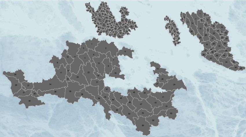
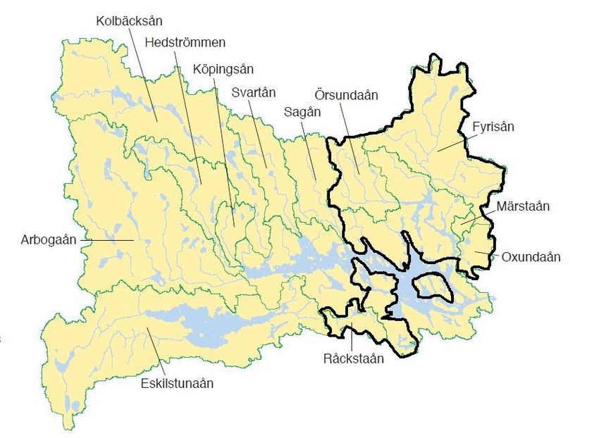
2. Background
The following chapter presents Lake Mälaren and nearby areas, with focus on the investigated
subbasins, as well as a review of microbial organisms relevant in the drinking water context.
Furthermore, projected future changes regarding climate change and socioeconomic development are
explained, and how the combined impact can affect Cryptosporidium and E. coli. Thereafter, several
recent studies on hydrological modeling of climate change and socioeconomic development are
reviewed. Lastly, there is a review of studies on modeling fecal contamination sources with focus on
methods and assumptions.

2.1 Lake Mälaren and nearby areas
Mälaren is the third largest lake in Sweden with its surface area of 1073 km². The catchment area is
approximately 22 600 km². The lake is surrounded by 23 municipalities (Mälarens vattenvårdsförbund,
n.d) which use Mälaren for drinking water supply, transportation, recreation and as a sewage recipient
(SMHI, 2021). There are five intakes for drinking water located in Mälaren which bring water to the
drinking treatment plants. The two largest drinking water treatment plants (DWTP) in the eastern part
are Lovö and Norsborg, which together supply 1 240 000 users with clean water. The third largest
DWTP is Görväln which treats water for 520 000 users (Johansson, 2014). The area around the lake is
dominated by urban areas, forests and bogs, fields and meadows and lakes. Mälaren has several large
tributaries which bring 80 % of the inflowing water to the lake. The primary outlet of Lake Mälaren is
Norrström, where the water is let out in the Baltic Sea (Sonesten, 2018).

 Figure 1. A map of the catchment area surrounding Lake Mälaren (Sonesten et al., 2013).

Since Lake Mälaren consists of many bays and islands it can be divided into several smaller delimited
water basins (Figure 2). The water quality is different due to natural causes between the basins,
difference in soil composition and water exchange. The lake can be seen as shallow since its mean depth
is 12.8 meters, and the depth is less than 3 m in approximately 20 % of the lake (Sonesten, 2018), but
the deepest part is up to 66 meters (SMHI, 2021). The difference in volume and in combination with
inflow of water makes retention time of the basins vary. Basin A in the western part of Figure 2 is
receiving almost 50 % of the inflowing water which results in a fast exchange of water. In the eastern
part where the larger and deeper basins are located, the exchange parameter and the retention time is

 3

important. Due to a slow water exchange and a long retention time the basins can function as a
sedimentation basin (Sonesten, 2018).

 Figure 2. Map of Lake Mälaren divided into smaller water basins (Sonesten et al., 2013).

The western part of the catchment area is different to the northern part regarding the composition of soil
which is a major cause to the imbalance of the chemical water composition between the basins. In the
northeast the moraine is relatively rich in nutrients and has a small amount of peat. The water is then
able to counteract acidification. However, in the northwestern part of the catchment area the conditions
are the opposite. The soil in the northwest has a low content of nutrition and a high proportion of peat
which makes the water poorly buffered (Sonesten, 2018).

The water quality of Lake Mälaren is vulnerable due to its surrounding environment. Leakages of
nitrogen, phosphorus and organic material from the sewage systems and arable and pasture lands are
creating undesirable disturbances of the aquatic life and environment (Ejhed, 2020). Disturbances such
as algae blooms can become a big problem which will both make the water low on oxygen but it can
also be a problem for the DWTPs (Norrvatten, n.d). The water from the surrounding activities does not
only contain nitrogen, phosphorus and organic material, it also contains microorganisms such as
pathogens and fecal indicators. The source of pathogens and indicators is often excreta and these
therefore seen as fecal contamination. The feces often come from humans, grazing animals and wildlife
(Johansson, 2014). The most common pathogens related to drinking water are Campylobacter, E. coli,
Salmonella, Shigella, Norovirus, Cryptosporidium, Entamoeba histolytica and Giardia (Säve-
Söderbergh, 2013), where E. coli often is seen as fecal indicator which can give an indication if there
are other fecal contaminants in the water (Ottosson, 2007).

 4

2.2 Microorganisms
Two common microbial organisms related to drinking water are Cryptosporidium and E. coli (Säve-
Söderbergh, 2013). Cryptosporidium is seen as a pathogen and E. coli is frequently seen as a fecal
indicator which can indicate if there are other pathogens present.

2.2.1 Cryptosporidium
Cryptosporidium is a protozoan which can cause infections in humans, cattles, lamb and other animals
(Folkhälsomyndigheten, 2019). The pathogens are excreted through oocysts in human and animal feces
and are transmitted via contaminated water or food (Folkhälsomyndigheten, 2019). Gastrointestinal
diseases caused by Cryptosporidium is a worldwide issue (Khalil et al., 2018). The severity of infection
varies among people, where infections in healthy adults usually resolve within a week, while infections
in severely immunocompromised human beings and infants and children of developing countries can be
life-threatening (Huang et al., 2004; WHO, 2017). In 2016, there were between 24 600 and 81 900 cases
of diarrheal related mortality globally for children under five years old, caused by Cryptosporidium,
with the majority of the cases (between 14000 and 50400) occurring in Western sub-Saharan Africa
(Khalil et al., 2018). Historical Cryptosporidium outbreaks in Sweden include events in Östersund in
2010 and Skellefteå in 2011 where 27 000 (Folkhälsomyndigheten, 2014a) and 20 000
(Folkhälsomyndigheten, 2014b) people respectively became infected by Cryptosporidium in the
drinking water.

Cryptosporidium can only reproduce inside a host, in other words a human or an animal
(Folkhälsomyndigheten, 2019), whereas other pathogens, for example Legionella can reproduce in
water (WHO, 2011). Cryptosporidium can however persist in water for several months (WHO, 2011),
which compared to other protozoa or bacteria is a long time (WHO, 2011). The protozoa will yet
gradually lose viability and ability to infect in water, and the decay rate is usually exponential (WHO,
2011).

Cryptosporidium reaching DWTPs is effectively removed with UV-treatment (WHO, 2011; Svenskt
Vatten, 2011) where 99.99% or more of the oocysts can be removed depending on the UV intensity
(Svenskt Vatten, 2011). Other treatment techniques include filtration which can remove up to 99.99%
(WHO, 2008) and coagulation/flocculation which can remove between 95-99.9% of the oocysts
(Svenskt Vatten, 2011). Cryptosporidium in wastewater treatment plants (WWTPs) is reduced by
sedimentation of oocysts bound to particles (Svenskt Vatten, 2011) and about 90-99% oocysts is
removed in four investigated Swedish WWTPs (Ottoson et al., 2006). Sufficient information on the
ability of Swedish WWTPs to reduce Cryptosporidium is however lacking (Socialstyrelsen, 2014).
There is also a lack of information on the ability of Swedish on-site wastewater treatment systems
(OWTSs) to reduce Cryptosporidium (Socialstyrelsen, 2014) as it is difficult to control outgoing
concentrations, and many households have insufficient OWTSs (Socialstyrelsen, 2014).

2.2.2 E. coli
Coliforms are members of bacteria groups which can be found in both human and animal feces. Coliform
bacteria, such as E. coli, are often used as indicators of the presence of potential sewage discharges or
diffuse sources such as grazing animals. The bacteria can indicate if there are possible presence of
disease-causing viruses, bacterias and protozoans which also are present in the human and animal
digestive systems (USEPA, n.d). A water without indicator bacteria does however not necessarily mean
that there are no other pathogens in the water, since indicators often have less survival time (Gertzell,
2017).

The persistence of E. coli in open environments such as soil, manure and water, is complex, and it
depends on physical, chemical and biological factors. Some groups of E. coli can resist pH-values of
2.5, that allows them to pass through the stomach, and if it invades the tissues it can cause death. The
ability of E. coli to grow and survive in an open environment is restricted. It is dependent on the

 5

environmental conditions and the availability of nutrients and energy sources, or else it will starve (Elsas
et.al, 2010). E. coli can be attached to suspended particles in open water and settle to bottom sediments
and survive for months, meanwhile in open water without suspended particles it does only survive for a
few days (Brinkmeyer et al., 2015).

2.3 Projected future changes
Projections regarding climate change and socioeconomic changes are presented in the following chapter.
The chapter also introduces the different representative concentration pathways (RCPs) and shared
socioeconomic pathways (SSPs) and how these can be combined.

2.3.1 Climate change scenarios
A major global challenge today is climate change. It is known to be caused by the greenhouse gases
(GHG), mostly from industrialization and economic growth (Schellnhuber, 2006). In line with the
growth of the economy, the world population has increased six times over the last two centuries, which
has caused an unsustainable global warming (Zhu & Peng, 2012). According to Schellnhuber (2006) the
global temperature has risen by 0.2°C since 1990 and there is evidence that most of it is due to human
activities. Projections are telling us that the warming of this century will be between 1.5 and 6°C as a
result of the increase of GHG (Schellnhuber, 2006).

The impacts of the ongoing and the forthcoming climate change can alter the hydrological cycle,
ecosystems and human health. According to the Intergovernmental Panel on Climate Change (2007)
(IPCC) in areas at high latitudes and in wet tropical climates, projections show that there may be an
increase by 10-40% of the annual average river runoff. But in dry areas the runoff can decrease by 10-
30%. The resilience in the ecosystems will be disturbed by the increased risk of floods, drought,
wildfires, land use change, pollution and overexploitation of resources. The health status of humans can
be decreased as a result of climate change. Deaths, diseases and injuries are expected to increase due to
heat, floods, fires, storms and droughts (IPCC, 2007).

To investigate various scenarios regarding climate change different representative concentration
pathways (RCP) have been derived by IPCC and the future projections are calculated from Global
Climate Models (GCM), see Table 1 (IPCC, 2014; SMHI, 2019). The RCPs are derived to support
research regarding the impact of GHG concentrations and emissions and potential policy responses (Kim
et.al, 2013). The RCPs are named by the levels of anthropogenic radiation which are projected before
the year 2100. Different radiative forcings mean different increases of GHG in the atmosphere. For
example the worst case, RCP8.5, means that there is a projected level of radiative force of 8.5 W/m2 up
to the year 2100. The radiative force is compared with levels at the pre-industrial time, mid 17th century
(SMHI, 2018).

 6

Table 1. Explanation of the four different RCPs derived by IPCC (SMHI, 2018).

The change in climate will have an impact on Sweden. It will cause higher temperatures and the levels
of precipitation will be increased, above all during the winter. The Swedish Meteorological and
Hydrological Institute (SMHI) have made simulations in the Stockholm area regarding the mean annual
temperature for year 2100 during the winter, for RCP4.5 it will increase with 3°C and for RCP8.5 with
6°C. The rise of temperature will result in a longer vegetation period and an expectation of more
consecutive days with a temperature above 20°C. The annual mean precipitation is expected to increase
with 20-30%, mostly during winter and spring. The amount of precipitation will be larger in the eastern
part of Stockholm area compared to the western. The increased number of consecutive days with higher
temperature will have an effect on the snow in forms of less snowfalls and less accumulation on the
ground (SMHI, 2015).

SMHI is estimating the discharge of water in the Stockholm area is expected to increase with 10% until
the mid-century and thereafter decrease. The streams around the area will be relatively unchanged except
for Oxundaån, where the flow will increase with 10%. As a result of the increased temperature, the
discharge of water during the winter period will increase drastically compared to the summer period
whereas it will decrease. The inflow during the winter with RCP4.5 and RCP8.5 will increase with 40-
75% from the levels of today to 2100, and during summer it will decrease with approximately 30%
(SMHI, 2015).

 7

2.3.2 Socioeconomic development scenarios
Socioeconomic development scenarios are used in climate research to provide plausible descriptions on
how the future may unfold with respect to socioeconomic factors such as birth rate, land use change,
consumption pattern and technological and economic development (Jin et al., 2018; Iqbal et al., 2018;
Islam et al., 2017; Zandersen et al., 2019). These factors can for example lead to population growth,
urbanization and agricultural intensification with increased microbial contamination of aquatic systems
as a consequence (Rose et al., 2001; Hofstra, 2011). The current level of scientific understanding in the
area is limited, and socioeconomic development may unfold in different and unpredictable ways
(Bartosova et al., 2019), meaning that the effect on for example water quality is uncertain, where
extending current socioeconomic trends may neglect unpredicted changes in current development from
policies, political developments or other events (Bartosova et al., 2019). Shared Socioeconomic
Pathways (SSPs) have therefore been developed, by scientific communities on behalf of IPCC (van
Vuuren et al., 2011) with five different development scenarios (SSP1-SSP5) used to reflect plausible
future developments (Table 2). The goal of applying scenarios is however not to create exact future
predictions but rather to discover different plausible developments to make more robust and informed
decisions (Berkhout et al., 2002).

Table 2. Summary of SSP narratives (O’Neill et al., 2017)

With the new development of SSPs, projections using both RCPs and SSPs are suggested (Van Vuuren
et al., 2012), where RCPs cover the climate forcing dimension of different possible futures (Van Vuuren
et al., 2011), while SSPs provide narratives of possible socioeconomic developments (O’Neill et al.,
2017). According to Berkhout et al. (2002) it is only possible to evaluate full climate change impact on
future societies when combining climate change factors with socioeconomic factors. Scientists
performing water quality assessments have therefore started to include socioeconomic scenarios (for
example change in land use, population, and technology) within their climate change scenarios. The
results show that the socioeconomic dimension has a substantial impact, and it may have a similar or

 8

even greater impact compared to climate change (Borris et al., 2016; Bartosova et al., 2019; Olesen et
al., 2019; Guo et al., 2020; Jin et al., 2018; Islam et al., 2018; Iqbal et al., 2019; Coffey et al., 2016).

There are different possible combinations of SSPs and RCPs depending on the amount of radiative
forcing that a specific SSP is expected to generate. SSP1 (with low mitigation and adaption challenges)
is consistent with RCP4.5 (as it adheres the “below 2°C target”) and the two are hence frequently
combined (Islam et al., 2018; Iqbal et al., 2018). SSP5 (high mitigation and low mitigation challenges)
is consistent with RCP8.5 and these two are therefore also frequently combined (Olesen et al., 2019; Jin
et al., 2018; Bartosova et al., 2019). SSP3 (high mitigation and adaption challenges) is also consistent
with RCP8.5 for developing countries, as it is unrealistic that low-income countries will contribute to
the amount of greenhouse gases generated in SSP5 (Islam et al., 2018; Iqbal et al., 2018). SSP2
(intermediate mitigation and adaptation challenges) can also be combined with RCP8.5 (Olesen et al.,
2019; Jin et al., 2018; Bartosova et al., 2019), but is only consistent up to the year 2050.

2.3.3 Effects of climatic and socioeconomic factors on microbial water quality
Climatic and socioeconomic factors can have an effect on Cryptosporidium and E. coli. Higher flows in
sewers generated from increased rainfall and population growth can for example contribute to more
sewer and WWTP overflows (Svenskt Vatten, 2011; Socialstyrelsen, 2014; Iqbal et.al, 2019). Increased
precipitation may further contribute to more surface runoff and therefore increased mobilisation and
higher concentrations of Cryptosporidium and E. coli (Socialstyrelsen, 2014; Pandey et.al, 2012;
Vermeulen and Hofstra, 2014). Droughts have also been associated with increased risks of
Cryptosporidium outbreaks (Lal and Konings, 2018), dry weather usually decreases the survival rate of
Cryptosporidium, nonetheless it may increase the concentrations of Cryptosporidium in relation to water
flow (Pozio, 2020). Dry weather also increases the amount of pathogens and indicators that can build
up on land before being mobilized by rain (Khan et al., 2015). Studies have found that the decay rate of
Cryptosporidium and E. coli is dependent on temperature, where increasing temperature is making the
decay rate increase (King and Monis, 2007; Vermeulen and Hofstra, 2014).

 9

2.4 Previous modeling of climate change and socioeconomic
development
As there are potential impacts of climate change and socioeconomic development on microorganisms
but also other pollutants, researchers have started to include projections of these factors in hydrological
modeling studies. The methods used in ten different studies (Table 3) to generate future projections,
mostly for hydrological modeling purposes, are described in chapter 2.4.1 and 2.4.2.

Table 3. Studies including SSP and RCP scenarios in their models.

2.4.1 Climate change
Investigated studies that have included climate change in water quality modeling have used downscaled
General Circulation Models (GCMs) to project future climate data, as the GCMs themselves are too
coarse and cannot provide high-resolution information for water resources and water quality studies
undertaken at a catchment scale (Jin et al., 2018). The number of climate scenarios, RCPs, varies
between studies where some studies use one, today most likely (Coffey et al., 2015) or worst case (Jin
et al., 2018), scenario. One study has included three scenarios to assess the impact of low, medium and
high greenhouse gas emissions developments (Guo et al., 2020). The most common method however,
also in line with IPCCs and Paris Accord recommendations for two climate futures (Whitehead et al.,
2019), is to use the RCP4.5 and RCP8.5 scenarios (Islam et al., 2018; Iqbal et al., 2019; Coffey et al.,
2016; Whitehead et al., 2019). Both scenarios are possible but also contrasting and can therefore frame
some of the uncertainties that are linked to modeling with future climate projections. Previous studies
have used RCPs mostly only for precipitation and temperature (Coffey et al., 2015; Coffey et al., 2016;
Guo et al., 2020; Whitehead et al., 2019; Jin et al., 2018; Iqbal et al., 2019) but also for sea level rise
(Islam et al., 2018).

 10

2.4.2 Socioeconomic development
Water quality modeling studies that have included socioeconomic development and have modeled
nutrients or pathogens (these are assumed to have similar contamination sources) have covered
socioeconomic changes in population, land use, livestock, wastewater treatment and manure
management (Coffey et al., 2015; Coffey et al., 2016; Coffey et al., 2020; Jin et al., 2018; Whitehead et
al., 2019; Islam et al., 2018; Iqbal et al., 2019; Bartosova et al., 2019; Olesen et al., 2019; Borris et al.,
2016). Quantitative changes for these factors have in previous studies mostly been made using relevant
sources and best judgement in line with the qualitative narratives presented in each SSP scenario, and/or
by directly using numerical projections presented in the IIASA SSP Database (IIASA, 2018). Variables
such as population growth and urban share for specific countries as well as land cover area (built-up
area, cropland, forest and pasture), demand and production of crops and livestock for specific world
regions are projected up to year 2100 in the IIASA SSP Database. Most studies have used two or more
socioeconomic scenarios in order to simulate different and contrasting possible pathways. Some studies
have moreover combined SSPs and RCPs in pairs (Islam et al., 2018; Iqbal et al., 2019) while other
studies have combined several SSPs with one (Olesen et al., 2019; Bartosova et al., 2019; Jin et al.,
2018) or several RCPs (Whitehead et al., 2019; Borris et al., 2016) as it is not certain which
socioeconomic scenario that will evolve and several SSPs may be consistent with one RCP (Van Vuuren
et al., 2013) especially for short term projections (up to 2050).

2.5 Previous modeling of fecal contamination
In order to simulate fecal contamination parameters in hydrological modeling programs, different fecal
contamination sources with accompanying contamination loads need to be defined. The methods used
in nine different studies (Table 4) to define these parameters are described in chapters 2.5.1, 2.5.2 and
2.5.3.

Table 4. Studies on modeling fecal contamination sources

2.5.1 Wastewater treatment plants (WWTPs)
Previous studies involving WWTPs have mostly used information on WWTP average discharges, from
measurements in WWTPs (Liu et al., 2019; Bergion et al., 2017; Coffey et al., 2010a; Coffey et al.,
2010b) or estimations from the total number of connected people (Thilakarathne et al., 2018; Bougeard
et al., 2011a) together with an assumed Cryptosporidium and/or E. coli concentration (Coffey et al.,
2010a.; Coffey et al., 2010b; Liu et al., 2019; Bergion, 2017) to calculate the total microbial load. To
calculate the load of Cryptosporidium and/or E. coli in the WWTP effluent a reduction efficiency has
been assumed (Coffey et al., 2010b; Coffey et al., 2010a; Bergion et al., 2017), one study has also
included direct measurements of Cryptosporidium loads in treated sewage (Liu et al., 2019). Both
methods resulted in similar Cryptosporidium loads.

 11

Overflows, from WWTPs and sewers, can be an important contributor to high pathogen concentrations
in water bodies (Svenskt Vatten, 2011; Socialstyrelsen, 2014), this has however only been included in
one study using reported daily means over a span of several years (Åström and Johansson, 2015). In one
of two simulated areas, mostly consisting of urban land, sewer overflows were an important contributor
to temporary peak concentrations of E. coli (Åström and Johansson, 2015).

2.5.2 On-site wastewater treatment systems (OWTSs)
Previous studies have used statistics to directly find the total number of OWTSs in the catchment area
(Coffey et al., 2010a; Coffey et al., 2010b; Coffey et al., 2013; Sowah et al., 2020) or by assuming that
addresses not connected to WWTPs in the catchment area have OWTSs (Thilakarathne et al., 2018; Liu
et al., 2019) or that each detached house contains one OWTS (Bergion et al., 2017). Based on the total
number of detached houses (SCB, n.d-a) and OWTSs (SCB, n.d-b) in Sweden there are more than twice
as many detached houses compared to OWTSs, hence the OWTS contribution of microorganisms may
vary greatly depending on used assumption.

The OWTS discharge has in previous studies been calculated by assuming an average household size
and a sewage discharge contribution from each person in the household (Coffey et al., 2010a; Coffey et
al., 2010b; Coffey et al., 2013; Bergion et al., 2017; Sowah et al., 2020; Thilakarathne et al., 2018; Liu
et al., 2019). A raw sewage sludge concentration of Cryptosporidium (Coffey et al., 2010b; Liu et al.,
2019; Bergion et al., 2017) and E. coli (Coffey et al., 2010a; Sowah et al., 2020; Bergion et al., 2017)
has been estimated together with an assumed OWTS treatment efficiency (Bergion et al., 2017; Coffey
et al., 2010a; Coffey et al., 2010b) and/or a septic tank failure rate (Thilakarathne et al., 2018; Sowah et
al., 2020; Coffey et al., 2010a; Coffey et al., 2010b; Coffey et al., 2013). The septic system water quality
database in SWAT only accounts for E. coli (Åström and Johansson, 2015) and nutrient loads (Sowah
et al., 2020). Hence, to, for example, include Cryptosporidium loads one need to assume a septic system
failure rate (Sowah et al., 2020) which is difficult to assume (Coffey et al,, 2010a; Coffey et al., 2010b).
Some studies have therefore recommended (Coffey et al., 2010a; Coffey et al., 2010b) or used (Bergion
et al., 2017) a continuous fertilisation management operation to model the influence from OWTSs as a
non-point source. This method however also has limitations as some OWTSs, for example OWTSs with
sand filters, should rather be characterised as point sources (Bergion et al., 2017).

2.5.3 Agriculture
In earlier studies, local statistics on livestock numbers have been used to find the amount of livestock in
investigated catchment areas (Coffey et al., 2010a; Coffey et al., 2010b; Coffey et al., 2013;
Thilakarathne et al., 2018; Liu et al., 2019; Sowah et al., 2020; Bergion et al., 2017). Liu et al. (2019)
have also used a reproduction factor for the existing livestock. The studies assume that grazing lasts for
a certain period where manure of grazing animals is directly deposited in the catchment area, either only
as a diffuse source on the ground (Coffey et al., 2010a; Coffey et al., 2010b; Bergion, 2017; Liu et al.,
2019; Thilakarathne et al., 2018), or also as a point source directly into streams (Coffey et al., 2013;
Coffey et al., 2015; Coffey et al., 2016; Sowah et al., 2020). Animal deposition directly into streams
have had considerable impact on the water quality in these studies (Coffey et al., 2013; Coffey et al.,
2015; Coffey et al., 2016; Sowah et al., 2020). When previous studies have included Cryptosporidium,
a prevalence scenario in livestock has also been assumed, which is varying depending on age, type of
animal and geographical location (Coffey et al., 2010b; Liu et al., 2019; Bergion et al., 2017). When
livestock are not grazing, for example, during winter months, it is assumed that the manure is stored and
later used as a fertilizer on arable land. Cryptosporidium and E. coli will degrade during this storing
period, hence some studies have included a “die-off” rate to take this into account (Bougeard et al.,
2011a; Tang et al., 2011; Liu et al., 2019). Bergion et al. (2017), did not include a “die-off” rate in stored
manure, and suggested that this could be one reason for high microorganism concentrations in their
model compared to observations.

 12

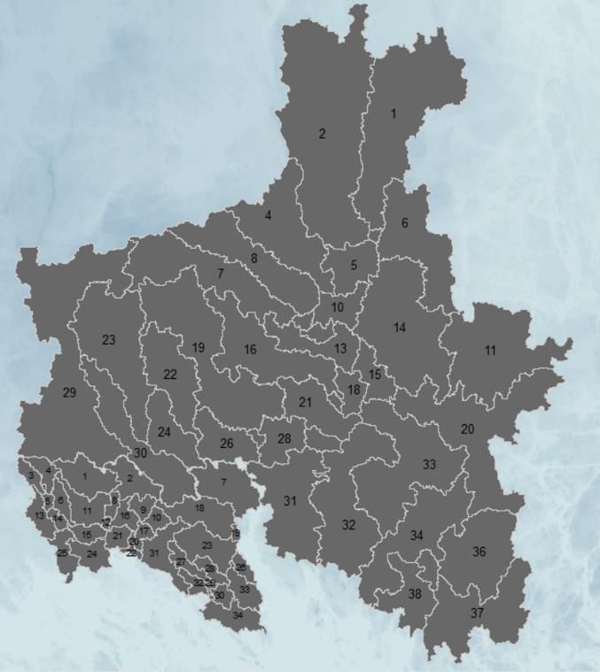
3. Method
The following chapter presents the study area and the setup of the SWAT-model which includes model
inputs and fecal contamination parameters. Furthermore, the sources of fecal contamination are
presented and quantified for the baseline scenario as well as the projected socioeconomic and climate
changes. At last, calibration and validation of the model are described.

3.1 Study area
The investigated area is the part of Norrström catchment area that drains water to Prästfjärden, Ekoln,
Skarven and Görväln (basin C, D and E in Figure 3) which potentially can affect the Görväln drinking
water treatment plant (Figure 4). Upstream areas with flow deviating from the Görväln DWTP (as
illustrated in Figure A1 in appendix) are outside of the scope of the thesis. The delineation of basins C,
D and E was performed and can be justified by hydrodynamic information, where in basin C the
retention time is 1.8 years (Sonesten et al., 2013), hence degradation and sedimentation will reduce the
impact of pathogens added to basin A and B. The delineated area was further interesting as it contains
several urban areas, for example Uppsala which is Sweden's fourth largest city, but also a lot of rural
areas and agriculture. Uppsala County, which covers the majority of the land in the delineated catchment
area, has had an increase in agricultural land between 1995-2010 unlike the rest of Sweden (Boverket,
2012).

 Figure 3. Different basins (basin A, B, C, D, E and F) in Mälaren (Sonesten et al., 2013).

 13

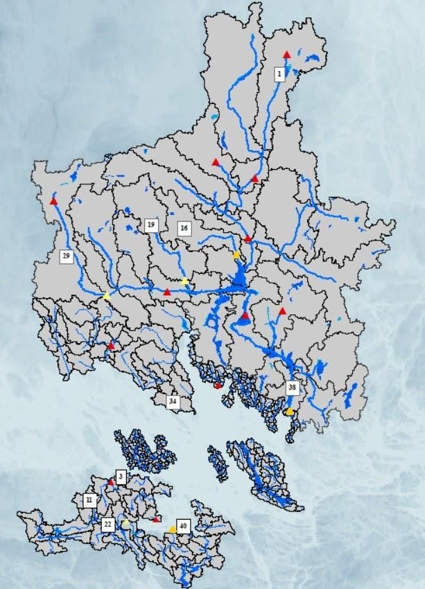
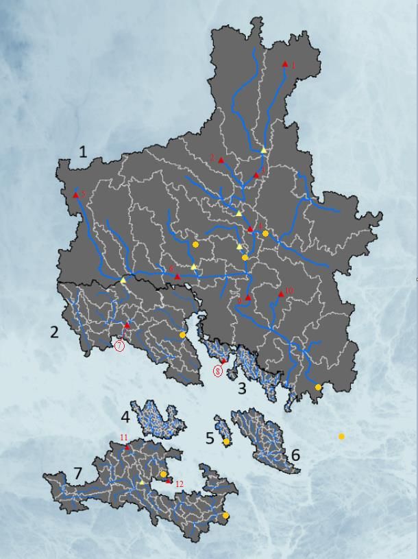
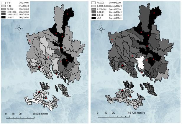
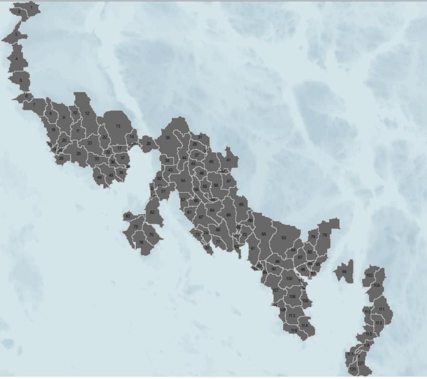
Görväln DWTP

Figure 4. Delineated catchment area (within the bold black boundaries). Map edited from Sonestet et al. (2013).

3.2 SWAT
Soil and Water Assessment Tool (SWAT) was formerly developed for the USDA Agricultural Research
Service to model hydrological changes. The tool was created to see how different land uses impact water
and sediments in larger catchment areas over time (Nietsch et al, 2011). The model includes rain, wind,
relative humidity, solar radiation, temperature, soil, hydrology, plant growth, pesticides and land
management. The catchment area in SWAT is divided into numerous subbasins, which later are sub-
divided into smaller Hydrologic Response Units (HRU) with similar physical properties and can be seen
as homogeneous. The HRUs consist of soil characteristics, land use and management (Gassman et al.,
2007).

3.2.1 Model setup
ArcSWAT version 2012.10.5.24 was used as a hydrological modeling program in this study. Seven
separate models were used in order to include the influence of all areas that are assumed to have a
pathogenic impact on Görväln DWTP (Figure 5). Of these models the Stäket catchment area (model 1)
was by far the largest while the islands of Strängnäs (model 4) and Ekerö (model 5 and 6) were the
smallest. The models were built with topographic conditions, geologic conditions, land use,
meteorological conditions, and point sources (wastewater treatment plants) to imitate realistic
hydrological conditions. Flow gauges were further added to the models to calibrate and validate the
hydrological conditions. The topographic conditions in the models were defined using a digital elevation
model (Table 5) retrieved from Swedish National Land Survey (Lantmäteriet, 2020). Geologic
conditions were defined using soil data (Table 5), that was used to describe different soil types, from
Geological Survey of Sweden (SGU, 2014) and a river burn in model (Table 5) from SMHI that was
used to delineate water courses (SMHI, 2016a). Land uses were defined using the “Corine Land Cover”
(Table 5) retrieved from Swedish National Land Survey (Lantmäteriet, 2019). Meteorological
conditions were defined using meteorological data (Table 5), between 2008 and 2020, retrieved from
SMHI (SMHI, n.d-a). Wastewater treatment plants (Table 5) were added as point sources using positions
from the VISS database (VISS, n.d). Flow gauges (Table 5) were added as subbasin outputs in the
models and the positions were retrieved from SMHI (SMHI, 2020a). Drainage basins and subbasins,
retrieved from SMHI, were moreover used to crop the digital elevation model to better fit each model
and reduce simulation time. The subbasins from SMHI were also used to see how well the produced
subbasins in the model corresponded in size to actual subbasins.

 14

Table 5. Input files used to describe hydrological conditions in the SWAT models or to calibrate and validate the
SWAT models.

The land uses defined in the Corine Land Cover (CLC) data were redefined to SWAT codes using
literature (El-Sadek and Ivrem, 2014; Kostra and Büttner, 2019) together with descriptions of the SWAT
codes. Soil data defined by the Geological Survey of Sweden was also redefined to SWAT codes using
literature (Johansson, 2014). Both the land use and soil shape data were merged and converted to raster
data in ArcMap. The slopes in the model were defined using three slope classes: 0-1%, 1-10% and 10-
99.99%. Six rain stations (Skjörby, Vattholma, Vittinge, Mariefred, Södertälje and Vallentuna), three
temperature stations (Uppsala, Stockholm and Södertälje), two wind stations (Adelsö and Stockholm)
and one relative humidity station (Adelsö) with data from 2008 to 2020 (SMHI, n.d-a) were used as
meteorological input. Solar radiation was assumed to be the same as the one present in the SWAT
weather database, this assumption was also made by Bergion et al. (2017).

 15

Figure 5. SWAT models in a collected representation. Red triangles represent WWTPs, yellow triangles
represent flow gauges, and orange circles represent meteorological stations. WWTPs also have numbers colored
 with red, connected to the WWTPs listed in Table 10. Numbers colored with black show the different models. In
 this report model 1 is named Stäket, model 2 Enköping, model 3 Stäket Under, model 4 Strängnäs Island, model
 5 and 6 Ekerö, and model 7 Strängnäs.

 16

3.2.2 Fecal contamination parameters
Cryptosporidium is assumed to be the persistent organism and E. coli is assumed to be the less persistent
organism in the models. The fecal contamination parameters in Table 6 were updated in the SWAT
models for both persistent and less persistent organisms.

Table 6. Fecal contamination parameters for SWAT.

 a) Bergion (2017)
 b) Tang et.al (2011)
 c) Coffey et.al (2010b)
 d) Bougeard et.al (2011b)
 e) Kim et.al (2010)
 f) Bougeard (2011a)

The decay rate in SWAT is based on the first order of Chick’s law (Baffaut & Sadeghi, 2010), see
Equation 1.

 = 0 − 20 ( −20) (Eq. 1)

 [count/100ml], the microbial concentration at time t; C0 [count/100ml], the initial microbial
concentration; K20 [day-1], first order of die-off rate at a temperature of 20°C; t [days], is exposure time;
 , temperature adjustment factor; T [°C], temperature.

 17

3.3 Fecal contamination sources
The following sub-chapter presents the different sources of fecal contamination which were a part of
the input in the SWAT model. The chapter on livestock and fertilization with manure describes the
contribution from pasture and arable land. The chapters on municipal wastewater treatment plants and
on-site wastewater treatment systems describe the contribution from urban land and detached house
properties.

3.3.1 Livestock and fertilization with manure
The contribution of microbial loads from the livestock in the catchment area is through fecal dropping,
which is assumed to be only on the pasture land during grazing. Another contribution is the stored feces
from the housing period which is used as manure fertilizer. The load from the pasture area was based
on the quantity of the livestock in each municipality. Each municipality's pasture area (Table AA1) and
the number of livestocks were gathered from Jordbruksverket (2020). The data on the available pasture
area and the number of the different animals were used to calculate a density of animals per hectare
(Table AA2). The fecal production was based on mean values for the different livestocks and the fecal
production per day was calculated, see Table 7. The fecal production for each type of livestock in each
municipality during grazing and housing is seen in Table 8. In the bracket called “cattle'' different kinds
of cows were included such as cows for production of milk, breeding, heifers, beef and calves under one
year. The bracket called “swines” includes boars and sows for breeding, pigs for slaughter above 20 kg
and piglets under 20 kg. The “poultry”-bracket combines hens for both layering and slaughter. The last
bracket “sheep” includes lambs, bags and ewes.

Table 7. Amount of feces produced by each type of livestock each day and days of grazing and housing.

 a) Atwill et.al (2012)
 b) Jordbruksverket (2021b)
 c) Jordbruksverket (2021c)
 d) Jordbruksverket (2021d)

 18

Table 8. Number of animals in each municipality, and the fecal production during grazing and housing.

 a) Jordbruksverket (2020)

To attain the fecal production per hectare for each municipality (Table 8) from grazing animals the
density was multiplied with the feces produced, which was later added in the fertilizer database in
SWAT. To consider the concentration of Cryptosporidium and E. coli in livestock feces a literature
study were made and the obtained values (Table 9) was added in the fertilizer database in SWAT. Since
only the infected organisms excrete pathogens the infected part of the population was important to
consider. Prevalence is the relationship between the infected and the healthy individuals in a population
(Åström, 2013). The relationship was considered through a factor to correct the concentration of
Cryptosporidium (Table 9). For the future scenarios it was assumed that the concentration of
Cryptosporidium and E. coli for each livestock and the prevalence of Cryptosporidium remains the
same.

Table 9. Concentration of E. coli and Cryptosporidium for each livestock and the prevalence of Cryptosporidium.

 a) Bergion (2017)
 b) Coffey et.al (2010b)
 c) Cox et.al (2005)
 d) Åström (2013)

The days when the livestocks is not outside, livestock is assumed to be housing and all feces are collected
and stored. It was assumed that the housing livestock produce the same amount of feces as when grazing
outside. During the manure storing period the concentration of E. coli in feces was assumed to decay
with a 3-log reduction rate (Bougard et.al, 2011) and the concentration of Cryptosporidium was reduced
with a die-off factor of 50 % (Tang et.al, 2011; Liu et.al, 2011). The stored manure (Table AA3) was
assumed to be fully applied on the arable land (Table AA1) as fertilizer during two periods, 1st March
and 1st October (Jordbruksverket, 2021a).

 19