Model evaluation of short-lived climate forcers for the Arctic Monitoring and Assessment Programme: a multi-species, multi-model study
←
→
Page content transcription
If your browser does not render page correctly, please read the page content below
Research article
Atmos. Chem. Phys., 22, 5775–5828, 2022
https://doi.org/10.5194/acp-22-5775-2022
© Author(s) 2022. This work is distributed under
the Creative Commons Attribution 4.0 License.

          Model evaluation of short-lived climate forcers for the
            Arctic Monitoring and Assessment Programme:
                   a multi-species, multi-model study
        Cynthia H. Whaley1 , Rashed Mahmood2,30 , Knut von Salzen1 , Barbara Winter3 , Sabine Eckhardt4 ,
           Stephen Arnold5 , Stephen Beagley31 , Silvia Becagli12 , Rong-You Chien7 , Jesper Christensen8 ,
             Sujay Manish Damani1 , Xinyi Dong7 , Konstantinos Eleftheriadis29 , Nikolaos Evangeliou4 ,
              Gregory Faluvegi9,10 , Mark Flanner11 , Joshua S. Fu7 , Michael Gauss12 , Fabio Giardi13 ,
       Wanmin Gong31 , Jens Liengaard Hjorth8 , Lin Huang6 , Ulas Im8 , Yugo Kanaya14 , Srinath Krishnan24 ,
           Zbigniew Klimont15 , Thomas Kühn16,17 , Joakim Langner18 , Kathy S. Law19 , Louis Marelle19 ,
       Andreas Massling8 , Dirk Olivié12 , Tatsuo Onishi19 , Naga Oshima20 , Yiran Peng21 , David A. Plummer3 ,
        Olga Popovicheva22 , Luca Pozzoli23 , Jean-Christophe Raut19 , Maria Sand24 , Laura N. Saunders25 ,
       Julia Schmale26 , Sangeeta Sharma6 , Ragnhild Bieltvedt Skeie24 , Henrik Skov8 , Fumikazu Taketani14 ,
          Manu A. Thomas18 , Rita Traversi13 , Kostas Tsigaridis9,10 , Svetlana Tsyro12 , Steven Turnock28,5 ,
       Vito Vitale23 , Kaley A. Walker25 , Minqi Wang21 , Duncan Watson-Parris27 , and Tahya Weiss-Gibbons1
            1 Canadian       Centre for Climate Modelling and Analysis, Environment and Climate Change Canada,
                                                          Victoria, BC, Canada
                        2 Department of Earth Science, Barcelona Supercomputing Center, Barcelona, Spain
               3 Canadian Centre for Climate Modelling and Analysis, Environment and Climate Change Canada,

                                                          Dorval, QC, Canada
         4 Department for Atmosphere and Climate, NILU – Norwegian Institute for Air Research, Kjeller, Norway
            5 Institute of Climate and Atmospheric Science, School of Earth and Environment, University of Leeds,

                                                         Leeds, United Kingdom
                   6 Climate Chemistry Measurements and Research, Environment and Climate Change Canada,

                                                          Toronto, ON, Canada
                                     7 University of Tennessee, Knoxville, Tennessee, United States
           8 Department of Environmental Science/Interdisciplinary Centre for Climate Change, Aarhus University,

                                                Frederiksborgvej 400, Roskilde, Denmark
                                   9 NASA Goddard Institute for Space Studies, New York, NY, USA
                        10 Center for Climate Systems Research, Columbia University, New York, NY, USA
              11 Department of Climate and Space Sciences and Engineering, University of Michigan, Ann Arbor,

                                                            MI, United States
           12 Division for Climate Modelling and Air Pollution, Norwegian Meteorological Institute, Oslo, Norway
                                  13 Department of Chemistry, University of Florence, Florence, Italy
               14 Research Institute for Global Change, Japan Agency for Marine-Earth Science and Technology,

                                                            Yokohama, Japan
                  15 Pollution Management Research group, International Institute for Applied Systems Analysis,

                                                           Laxenburg, Austria
                          16 Department of Applied Physics, University of Eastern Finland, Kuopio, Finland
             17 Atmospheric Research Centre of Eastern Finland, Finnish Meteorological Institute, Kuopio, Finland
                              18 Swedish Meteorological and Hydrological Institute, Norrköping, Sweden
                                     19 LATMOS, CNRS-UVSQ-Sorbonne Université, Paris, France
                        20 Meteorological Research Institute, Japan Meteorological Agency, Tsukuba, Japan
        21 Department of Earth System Science, Ministry of Education Key Laboratory for Earth System Modeling,

                               Institute for Global Change Studies, Tsinghua University, Beijing, China

Published by Copernicus Publications on behalf of the European Geosciences Union.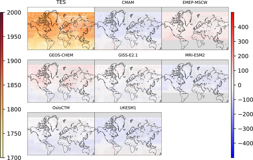
5776                                                                       C. H. Whaley et al.: AMAP SLCF model evaluation

                    22 Skobeltsyn   Institute of Nuclear Physics, Moscow State University, Moscow, Russia
                                 23 European     Commission, Joint Research Centre, Ispra, Italy
                    24 CICERO Center for International Climate and Environmental Research, Oslo, Norway
                              25 Department of Physics, University of Toronto, Toronto, ON, Canada
                   26 Extreme Environments Research Laboratory, École Polytechnique Fédérale de Lausanne,

                                                      Lausanne, Switzerland
         27 Atmospheric, Oceanic and Planetary Physics, Department of Physics, University of Oxford, Oxford, UK
                                              28 Met Office Hadley Centre, Exeter, UK
          29 Institute of Nuclear and Radiological Science & Technology, Energy & Safety N.C.S.R. “Demokritos”,

                                                           Attiki, Greece
                           30 Department of Geography, University of Montreal, Montreal, QC, Canada
         31 Air Quality Modelling and Integration, Environment and Climate Change Canada, Toronto, ON, Canada

                              Correspondence: Cynthia H. Whaley (cynthia.whaley@ec.gc.ca)

                               Received: 24 November 2021 – Discussion started: 26 November 2021
                            Revised: 23 March 2022 – Accepted: 24 March 2022 – Published: 4 May 2022

       Abstract. While carbon dioxide is the main cause for global warming, modeling short-lived climate forcers
       (SLCFs) such as methane, ozone, and particles in the Arctic allows us to simulate near-term climate and health
       impacts for a sensitive, pristine region that is warming at 3 times the global rate. Atmospheric modeling is critical
       for understanding the long-range transport of pollutants to the Arctic, as well as the abundance and distribution
       of SLCFs throughout the Arctic atmosphere. Modeling is also used as a tool to determine SLCF impacts on
       climate and health in the present and in future emissions scenarios.
          In this study, we evaluate 18 state-of-the-art atmospheric and Earth system models by assessing their represen-
       tation of Arctic and Northern Hemisphere atmospheric SLCF distributions, considering a wide range of different
       chemical species (methane, tropospheric ozone and its precursors, black carbon, sulfate, organic aerosol, and
       particulate matter) and multiple observational datasets. Model simulations over 4 years (2008–2009 and 2014–
       2015) conducted for the 2022 Arctic Monitoring and Assessment Programme (AMAP) SLCF assessment report
       are thoroughly evaluated against satellite, ground, ship, and aircraft-based observations. The annual means, sea-
       sonal cycles, and 3-D distributions of SLCFs were evaluated using several metrics, such as absolute and percent
       model biases and correlation coefficients. The results show a large range in model performance, with no one
       particular model or model type performing well for all regions and all SLCF species. The multi-model mean
       (mmm) was able to represent the general features of SLCFs in the Arctic and had the best overall performance.
       For the SLCFs with the greatest radiative impact (CH4 , O3 , BC, and SO2−   4 ), the mmm was within ±25 % of the
       measurements across the Northern Hemisphere. Therefore, we recommend a multi-model ensemble be used for
       simulating climate and health impacts of SLCFs.
          Of the SLCFs in our study, model biases were smallest for CH4 and greatest for OA. For most SLCFs, model
       biases skewed from positive to negative with increasing latitude. Our analysis suggests that vertical mixing,
       long-range transport, deposition, and wildfires remain highly uncertain processes. These processes need better
       representation within atmospheric models to improve their simulation of SLCFs in the Arctic environment. As
       model development proceeds in these areas, we highly recommend that the vertical and 3-D distribution of
       SLCFs be evaluated, as that information is critical to improving the uncertain processes in models.

1   Introduction                                                    including radiative forcings by short-lived climate forcers
                                                                    (SLCFs), such as methane, black carbon, and tropospheric
The Arctic atmosphere is warming 3 times more quickly               ozone (AMAP, 2015a, b, 2022). The remote pristine Arc-
than the global average (Bush and Lemmen, 2019; NOAA,               tic environment is sensitive to the long-range transport of at-
2020; AMAP, 2021; IPCC, 2021). Arctic warming is a man-             mospheric pollutants and deposition (Schmale et al., 2021).
ifestation of global warming, and the main driver for this is       At the same time, it is difficult to carry out in situ measure-
the increasing carbon dioxide (CO2 ) radiative forcing (IPCC,       ments (Nguyen et al., 2016; Freud et al., 2017) and satel-
2021). Arctic warming is amplified by sea ice and snow feed-        lite observations over the Arctic. The majority of the Arctic
backs and affected by local radiative forcings in the Arctic,       surface is ocean covered with sea ice that is usually adrift

Atmos. Chem. Phys., 22, 5775–5828, 2022                                              https://doi.org/10.5194/acp-22-5775-2022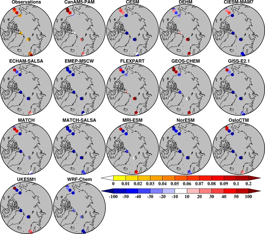
C. H. Whaley et al.: AMAP SLCF model evaluation                                                                             5777

for most of the year. The Arctic environment is also harsh.         out of scope are the models’ simulations of aerosol optical
These aspects have historically kept surface-based measure-         properties and cloud properties (e.g., cloud fraction, cloud
ments sparse. The overwhelming majority of the satellite ob-        droplet number concentration, cloud scavenging), though
servations either depend on the visible spectrum, are limited       those parameters do have a large impact on climate and a
by the presence of clouds, or have very low sensitivity in the      tight relationship with some SLCFs. Their initial evaluation
lower troposphere where the atmospheric processes mainly            can be found in AMAP (2022) (chap. 7). Estimates of effec-
determine the fate of the pollutants. Many satellite measure-       tive radiative forcings of SLCFs in the Arctic by the AMAP
ments also do not have good coverage in the Arctic, given           participating models are also provided elsewhere (Oshima
their orbital parameters or problems measuring areas with           et al., 2020).
high albedo (Beer, 2006).                                              The next section summarizes the models used in this study,
   Modeling the Arctic atmosphere comes with its own chal-          with more information in the Appendix. Section 3 summa-
lenges due to extreme meteorological conditions, its great          rizes the measurements used for model evaluation. Section 4
distance from major global pollution sources, poorly known          presents our model evaluation for each SLCF species, fol-
local emissions, high gradients in physical and chemical            lowed by a summary of all SLCFs. Finally, Sect. 5 is the
fields, and a singularity in some model grids at the pole.          conclusion where the questions posed above are answered.
Models have been improving in the last 2 decades, but many
models still have inaccurate results in the Arctic (Shindell        2     Models
et al., 2008; Eckhardt et al., 2015; Emmons et al., 2015;
Sand et al., 2017; Marelle et al., 2018). That said, there          In this section we briefly describe the models used for the
has recently been a number of improvements in numerous              AMAP SLCF study and refer the reader to Appendix A for
models that have allowed for better representation of certain       individual model descriptions and further information. All
processes (Morgenstern et al., 2017; Emmons et al., 2020a;          models were run globally with the same anthropogenic emis-
Swart et al., 2019; Holopainen et al., 2020; Im et al., 2021). In   sions dataset (see Sect. 2.1), and most were run for the years
this study, model simulations for the 2021 Arctic Monitoring        2008–2009 (as was done for the 2015 AMAP assessment re-
and Assessment Programme (AMAP) SLCF assessment re-                 port) and 2014–2015 (to evaluate more recent model results)
port (AMAP, 2022) have been thoroughly evaluated by com-            inclusive for this evaluation, as these were years with nu-
parison to several freely available observational datasets in       merous Arctic measurements. Unless otherwise indicated, all
the Northern Hemisphere and assessed in more detail in the          model output was monthly-averaged.
Arctic. In order to support the integrated assessment of cli-          The models used for this study are summarized in Ta-
mate and human health for AMAP, 6 SLCF species (methane             ble 1. As is shown in the table, not all models provided
– CH4 , ozone – O3 , black carbon – BC, sulfate – SO2−    4 , or-   all SLCF species, and not all models provided all 4 years.
ganic aerosol – OA, and fine particulate matter – PM2.5 ) and       There were eight chemical transport models (CTMs), two
2 O3 precursors (carbon monoxide – CO; nitrogen dioxide             chemistry–climate models (CCMs), three global climate
– NO2 ) from 18 atmospheric or Earth system models are              models (GCMs), and five Earth system models (ESMs).
compared to numerous observational datasets (from three             Many models used specified or nudged meteorology, which
satellite instruments, seven monitoring networks, and nine          allows the day-to-day variability of the model meteorology to
measurement campaigns) for 4 years (2008–2009 and 2014–             be more closely aligned with the historical evolution of the
2015), with the goal of answering the following questions.          atmosphere than occurs in a free-running model. The ERA-
  1. How well do the AMAP SLCF models perform in the                Interim reanalysis was the most commonly used meteorology
     context of measurements and their associated uncer-            (in 7 out of 18 models), but some were free-running (simulat-
     tainty?                                                        ing their own meteorology) and some used other reanalysis
                                                                    products (Table 1).
  – What do the best-performing models have in common?
  – Are there regional patterns in the model biases?                2.1    Emissions

  – Are there patterns in the model biases between SLCF             All models used the same anthropogenic emissions dataset,
    species?                                                        which is called ECLIPSE (Evaluating the Climate and Air
                                                                    Quality Impacts of Short-Lived Pollutants) v6B. These emis-
  2. How does the model performance impact model appli-             sions were created using the IIASA-GAINS (International
     cations, such as simulated climate and health impacts?         Institute for Applied Systems Analysis – Greenhouse gas
                                                                    – Air pollution Interactions and Synergies) model (Amann
  3. What processes should be improved or studied further
                                                                    et al., 2011; Klimont et al., 2017; Höglund-Isaksson et al.,
     for better model performance?
                                                                    2020), which provides emissions of long-lived greenhouse
 Out of scope of this study are any sensitivity tests by the        gases and shorter-lived species in a consistent framework.
models to assess different components of model errors. Also         These historical emissions were provided for the years 1990

https://doi.org/10.5194/acp-22-5775-2022                                           Atmos. Chem. Phys., 22, 5775–5828, 2022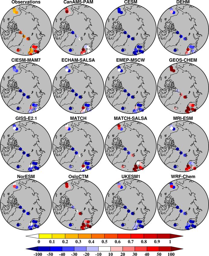
Table 1. Summary of models used in this study. GCM: global climate model, CCM: chemistry–climate model, ESM: Earth system model, CTM: chemical transport model.
C. H. Whaley et al.: AMAP SLCF model evaluation
https://doi.org/10.5194/acp-22-5775-2022
Name Type Meteorology Simulation period SLCF output Primary reference(s)
CanAM5-PAM GCM nudged to ERA- 1990–2015 BC, SO42− , OA, PM2.5 , von Salzen et al. (2000); von Salzen (2006); von Salzen et al. (2013)
Interim reanalysis AOD, AAOD, AE Ma et al. (2008); Peng et al. (2012); Mahmood et al. (2016, 2019)
CESM2.0 ESM free-running 2008–2009, 2014–2015 O3 , CO, NO2 , BC, Danabasoglu et al. (2020)
SO42− , OA, PM2.5 , AOD, Liu et al. (2016)
AAOD, AE
CIESM-MAM7 GCM nudged to ERA- 1990–2015 BC, SO42− , OA, PM2.5 , Lin et al. (2020); Liu et al. (2012)
Interim reanalysis AOD
CMAM CCM nudged to ERA- 1990–2015 O3 , CO, NO2 , CH4 Jonsson et al. (2004)
Interim reanalysis Scinocca et al. (2008)
DEHM CTM nudged to ERA- 1990–2015 O3 , CO, NO2 , CH4 , Christensen (1997); Brandt et al. (2012); Massling et al. (2015)
Interim reanalysis BC, SO42− , OA, PM2.5 ,
AOD, AAOD, AE
ECHAM6-SALSA GCM nudged to ERA- 2008–2009, 2014–2015 BC, SO42− , OA, PM2.5 , Tegen et al. (2019); Schultz et al. (2018); Kokkola et al. (2018)
Interim reanalysis AOD, AAOD, AE
EMEP MSC-W CTM driven by 3-hourly 1990–2015 O3 , CO, NO2 , CH4 , Simpson et al. (2012, 2019)
ECMWF met BC, SO42− , OA, PM2.5 , AOD
FLEXPART Lagrangian CTM driven by 3-hourly 2014–2015 BC, SO42− Pisso et al. (2019)
ECMWF met
GEM-MACH online CTM driven by GEM 2015 O3 , CO, NO2 , BC, Moran et al. (2018)
numerical forecast SO42− , OA, PM2.5 Makar et al. (2015b, a); Gong et al. (2015)
GEOS-Chem CTM Driven by GEOS 2008–2009, 2014–2015 O3 , CO, NO2 , CH4 , Bey et al. (2001)
meteorology BC, SO42− , OA, PM2.5 ,
AOD, AAOD, AE
GISS-E2.1 ESM nudged to NCEP 1990–2015 O3 , CO, NO2 , CH4 , Kelley et al. (2020); Miller et al. (2021); Bauer et al. (2020)
reanalysis BC, SO42− , OA, PM2.5 ,
AOD, AAOD, AE
Atmos. Chem. Phys., 22, 5775–5828, 2022
MATCH CTM ERA-Interim 2008–2009, 2014–2015 O3 , CO, NO2 , BC, Robertson et al. (1999)
reanalysis SO42− , OA, PM2.5 , AOD, AAOD, AE
MATCH-SALSA-RCA4 CCM RCA4 2008–2009, 2014–2015 O3 , CO, NO2 , BC, Robertson et al. (1999); Andersson et al. (2007); Kokkola et al. (2008)
SO42− , OA, PM2.5 , AOD, AAOD, AE
MRI-ESM2 ESM nudged to JRA55 1990–2015 O3 , CO, NO2 , CH4 , Yukimoto et al. (2019); Kawai et al. (2019); Oshima et al. (2020)
reanalysis BC, SO42− , OA, PM2.5 ,
AOD, AAOD
NorESM1-happi ESM free-running 2008–2009, 2014–2015 BC, SO42− , OA, AOD, Bentsen et al. (2013); Iversen et al. (2013); Gent et al. (2011)
AAOD, AE Graff et al. (2019)
Oslo-CTM CTM driven by 3-hourly 2008–2009, 2014–2015 O3 , CO, NO2 , CH4 , Søvde et al. (2012); Lund et al. (2018a)
ECMWF meteorology BC, SO42− , OA, PM2.5
UKESM1 CCM & ESM nudged to ERA- 1990–2015 O3 , CO, NO2 , CH4 , Sellar et al. (2019); Kuhlbrodt et al. (2018); Williams et al. (2018)
Interim reanalysis BC, SO42− , OA, PM2.5 ,
AOD, AAOD, AE
5778
WRF-Chem CCM & CTM nudged to NCEP FNL 2014–2015 O3 , CO, NO2 , BC, SO42− , Marelle et al. (2017, 2018)
reanalysis OA, PM2.5 , AOD, AAOD, AE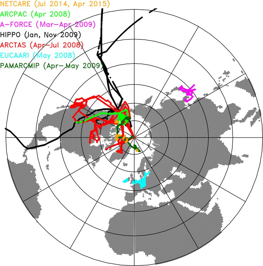
C. H. Whaley et al.: AMAP SLCF model evaluation                                                                              5779

to 2015 at 5-year intervals, as well as the years 2008–2009        2.2.1   Methane
and 2014. Those models that simulated the 1990–2015 time
                                                                   All participating models that provided CH4 output prescribed
period linearly interpolated the emissions for the years in
                                                                   CH4 concentrations based on box model results from Olivié
between. The ECLIPSEv6b emissions include many pollu-
                                                                   et al. (2021) for 2015 and from Meinshausen et al. (2017)
tants, such as CH4 , CO, NOx , BC, and SO2 . They include
                                                                   for years prior to 2015. The former utilized the ECLIPSE
the significant sulfur emission reductions that have taken
                                                                   v6B anthropogenic CH4 emissions (Sect. 2.1), along with
place since the 1980s (Grennfelt et al., 2020). Global anthro-
                                                                   assumptions for the natural emissions (Olivié et al., 2021;
pogenic BC emissions are estimated to be 6.5 Tg in 2010 and
                                                                   Prather et al., 2012), to provide as input to models’ surface or
5.9 Tg in 2020, and global anthropogenic SO2 emissions are
                                                                   boundary layer CH4 concentrations. Models then allow CH4
estimated to be 90 Tg in 2010 but declined significantly over
                                                                   to take part in photochemical processes, such as the produc-
the subsequent decade to 50 Tg (AMAP, 2022). The reduc-
                                                                   tion of tropospheric O3 .
tions are mainly due to stringent emissions standards in the
energy and industrial sectors, as well as reduced coal use in
the residential sector (AMAP, 2022). Global anthropogenic          2.2.2   Tropospheric chemistry
methane emissions were 340 Tg in 2015 and 350 Tg in 2020,          There is a wide range of tropospheric gas-phase chem-
and they are expected to continue to increase, unlike BC and       istry implemented in the models. Air-quality-focused mod-
SO2 . The largest methane sources in 2015 were agriculture         els, such as DEHM, EMEP MSC-W, GEM-MACH, GEOS-
(42 % of total emissions), oil and gas (extraction and distribu-   Chem, MATCH, and WRF-Chem, have detailed HOx –
tion) (18 %), waste (18 %), and energy production (including       NOx –hydrocarbon O3 chemistry, with speciated volatile or-
coal mining) (16 %) (AMAP, 2022; Höglund-Isaksson et al.,          ganic compounds (VOCs) and secondary aerosol forma-
2020). CO and NOx emissions have been declining steadily           tion. The GISS-E2.1, MRI-ESM2, and UKESM1 ESMs
and are expected to continue declining in the future.              also use this level of tropospheric chemistry. In con-
   In comparison to the CMIP6 emissions (Hoesly et al.,            trast, climate-focused models like CanAM5-PAM, CIESM-
2018), ECLIPSEv6b emissions have additionally taken into           MAM7, ECHAM-SALSA, and NorESM1 contain bare min-
account the recent declines in emissions from Asia of SO2 ,        imum gas-phase chemistry and use prescribed O3 fields (e.g.,
BC, and NOx due to recent control measures, whereas those          CanAM5-PAM uses CMAM climatological O3 fields). The
declines in the CMIP6 emissions were unrealistically small         CCMs are somewhere in between, with simplified tropo-
(Wang et al., 2021; von Salzen et al., 2022). The inclusion of     spheric and stratospheric chemistry so that they could be run
emissions from the flaring sector in Russia was a significant      for longer time periods. For example, CMAM’s tropospheric
improvement, which was not present in the previous version         chemistry consists only of CH4 –NOx –O3 chemistry, with no
of ECLIPSE emissions that was used in the AMAP (2015a)             VOCs.
report.
   For non-agricultural fire emissions, many models utilized
the CMIP6 fire emissions, which are based on monthly               2.2.3   Stratospheric chemistry
GFED (Global Fire Emissions Database) v4.1 (van Marle              Only a subset of the participating models have a fully
et al., 2017). About half of the models included volcanic          simulated stratosphere. CMAM, MRI-ESM2, GISS-E2.1,
emissions or stratospheric aerosol concentrations from the         OsloCTM, and UKESM1 contain a relatively complete de-
CMIP6 dataset (Thomason et al., 2018) or other sources,            scription of the HOx , NOx , Clx , and Brx chemistry that
and the other half did not include volcanic emissions, which       controls stratospheric ozone along with the longer-lived
mainly impact SO2 and thus modeled SO2−      4 . The emissions     source gases such as CH4 , N2 O, and chlorofluorocarbons
from the October to December 2014 Honoluraun volcano               (CFCs). Other models have a simplified stratosphere, such as
eruption (Gíslason et al., 2015; Twigg et al., 2016; Ilyinskaya    GEOS-Chem, which has a linearized stratospheric chemistry
et al., 2017) were included by six models in a separate set of     scheme (Linoz, McLinden et al., 2000), and WRF-Chem,
simulations. Similar differences in biogenic and agricultural      which specifies stratospheric concentrations from climatolo-
waste emissions appear in these model simulations, and all         gies – both of which do not simulate stratospheric chem-
are summarized in Table 2.                                         istry. Finally, several models have no stratosphere or strato-
                                                                   spheric chemistry at all (e.g., CIESM-MAM7, GEM-MACH,
2.2   Chemistry                                                    DEHM, and EMEP MSC-W).
This section contains a summary of models’ chemistry
schemes, and we refer the reader to Appendix A and refer-          2.2.4   Aerosols
ences therein for more details.                                    Most models contain speciated aerosols: mineral dust (also
                                                                   known as crustal material), sea salt, BC, OA (sometimes sep-
                                                                   arated into primary and secondary), SO2−                  −
                                                                                                              4 , nitrate (NO3 ),
                                                                                       +
                                                                   and ammonium (NH4 ). However, some, like CanAM5-PAM

https://doi.org/10.5194/acp-22-5775-2022                                           Atmos. Chem. Phys., 22, 5775–5828, 2022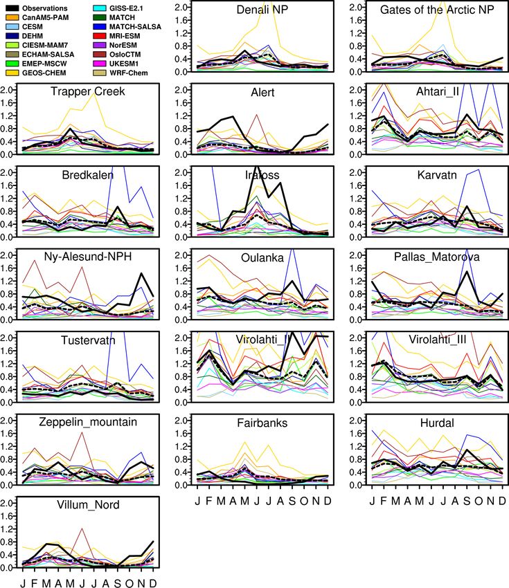
C. H. Whaley et al.: AMAP SLCF model evaluation

                                                                                                                                                                                                                               https://doi.org/10.5194/acp-22-5775-2022
                                                  Table 2. Summary of emissions used in the models
                                                   Model                   Biogenic                                Volcanic                                          Forest fire                Agricultural waste
                                                                                                                                                                                                burning
                                                   CanAM5-PAM              none                                    specified climatological emissions                CMIP6                      ECLIPSEv6b
                                                                                                                   and CMIP6 stratospheric aerosol
                                                   CESM2.0                 MEGANv2.1                               CMIP6                                             CMIP6                      ECLIPSEv6b
                                                   CIESM-MAM7              none                                    CMIP6                                             CMIP6                      ECLIPSEv6b
                                                   CMAM                    none                                    none                                              CMIP6                      ECLIPSEv6b
                                                   DEHM                    MEGANv2                                 none                                              GFAS                       ECLIPSEv6b
                                                   ECHAM6-SALSA            GEIA inventory                          3-D emissions based                               CMIP6                      ECLIPSEv6b
                                                                           (PM only)                               on AeroCom III
                                                   EMEP MSC-W              EMEP scheme                             degassing from Ethna, Stromboli,                  FINN                       ECLIPSEv6b
                                                                           Simpson et al. (2012)                   Eyjafjallajökull (2010), Grimsvotn (2011),        Wiedinmyer et al. (2011)
                                                                                                                   Holuhraun (2014, 2015)
                                                   FLEXPART                none                                    none                                              CMIP6                      ECLIPSEv6b
                                                   GEM-MACH                BEIS v3.09                              none                                              CFFEPS                     ECLIPSEv6b outside
                                                                                                                                                                                                NA, US NEI and Canadian APEI
                                                   GEOS-Chem               MEGANv2.1 with updates                  NASA/GMAO                                         GFEDv4.1                   ECLIPSEv6b
                                                   GISS-E2.1               Guenther et al. (2012) isoprene,        AeroCom                                           CMIP6                      ECLIPSEv6b
                                                                           ORCHIDEE terpenes, online DMS,
                                                                           SS and dust

                                                                                                                                                                                                                               Atmos. Chem. Phys., 22, 5775–5828, 2022
                                                   MATCH                   MEGANv2                                 climatological and Honoluraun                     CMIP6                      ECLIPSEv6b
                                                   MATCH-SALSA-RCA4        MEGANv                                  climatological and Honoluraun                     CMIP6                      ECLIPSEv6b
                                                   MRI-ESM2                Horowitz et al. (2003)                  CMIP6 stratospheric aerosol and Honoluraun        CMIP6                      ECLIPSEv6b
                                                   NorESM1-happi           Dentener et al. (2006)                  CMIP6                                             CMIP6                      ECLIPSEv6b
                                                   Oslo-CTM                MEGAN-MACC at 2010                      AeroCom (Dentener et al., 2006)                   GFEDv4                     ECLIPSEv6b
                                                                                                                   Andres and Kasgnoc (1998); Halmer et al. (2002)
                                                   UKESM1                  isoprene and monoterpenes interactive   climatology, CMIP6                                CMIP6                      CMIP6
                                                                           with land surface vegetation scheme
                                                   WRF-Chem                MEGANv2.1                               none                                              GFED                       ECLIPSEv6b
5780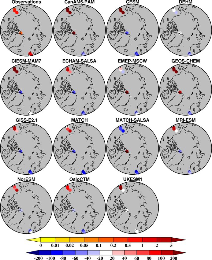
C. H. Whaley et al.: AMAP SLCF model evaluation                                                                                 5781

and UKESM1, do not simulate NO−               +
                                    3 and NH4 , but assume            portional to the NO concentration. NO2 measurements are
                             2−         2−
all is in the form (NH4 )2 SO4 . OA, SO4 , NO−  3 , and NH4
                                                           +          approximated using its thermal reduction to NO by a heated
are involved in chemical reactions interacting with the gas-          (350◦ C) molybdenum converter (Bauguitte, 2014). Note that
phase chemistry. Aerosol size distributions are either pre-           this method has an estimated bias of about 5 %–20 % be-
scribed or discretized into lognormal modes or size sec-              cause of sensitivity to other oxidized nitrogen species, and
tions. How the aerosol size distribution varies in space and          this has not been corrected for. The bias is on the lower end
time depends on many different processes, including emis-             for high-NOx conditions and in the low-NOx Arctic can be
sion, aerosol microphysics, aerosol–cloud interactions, and           up to 100 % uncertainty.
removal. How these processes are parameterized depends on
the model, and we refer the reader to the Appendix and the            3.1.3   BC and OA
references therein for more detail.
                                                                      There are various BC measurement methods exploiting dif-
                                                                      ferent properties of BC and thus measuring different quan-
3     Measurements                                                    tities (Petzold et al., 2013): elemental carbon (EC) deter-
                                                                      mined by thermal and/or thermal–optical methods, equiva-
We have utilized many freely available observational datasets         lent BC (eBC) by optical absorption methods, and refrac-
of SLCFs to evaluate the models. General descriptions are             tory BC (rBC) by incandescence methods. Table B1 in Ap-
given below under the broad headings of surface monitoring,           pendix B lists the different measurement techniques and in-
satellite, and campaign datasets, and there is some additional        struments that the different monitoring networks and individ-
information in Appendix B.                                            ual Arctic monitoring stations use. As BC emission invento-
                                                                      ries, including ECLIPSEv6b, are mainly based on emission
3.1     Surface monitoring datasets                                   factors derived from thermal and/or thermal–optical meth-
                                                                      ods, modeled BC is consequently representative of EC.
3.1.1    CH4 and O3                                                       The different types of BC measurements (EC, eBC, and
Global surface CH4 measurements were obtained from the                rBC) usually agree with each other within a factor of 2
World Data Centre for Greenhouse Gases (WDCGG). These                 (AMAP, 2022; Pileci et al., 2021). However, it has been
measurements were made via gas chromatography, which                  shown that, as the aerosol ages, the complex state of mix-
has a < 1 % uncertainty range. Surface in situ O3 measure-            ing of BC particles causes eBC to increase relative to EC
ments are typically made via various types of UV absorp-              (Zanatta et al., 2018). The absorption and scattering cross
tion monitors, employing the Beer–Lambert law to relate               sections of coated BC particles vary by more than a factor of
UV absorption of O3 at 254 nm directly to the concentra-              2 due to different coating structures. He et al. (2015) found an
tion of O3 in the sample air (e.g., Bauguitte, 2014), which           increase of 20 %–250 % in absorption during aging, signifi-
have approximately a 3 % or 1–2 ppbv uncertainty range. We            cantly depending on coating morphology and aging stages.
obtained surface O3 measurements from various networks:               Thus, this complexity impacts model–measurement compar-
the National Air Pollutant Surveillance Program (NAPS) and            isons at remote Arctic locations where one would expect eBC
the Canadian Pollutant Monitoring Network (CAPMON) for                to have a high, positive uncertainty.
Canada, the Chemical Speciation Network (CSN) for the US,                 We obtained BC from the Canadian Aerosol Baseline
the Beijing Air Quality and Hong Kong Environmental Pro-              Measurement (CABM) network for Canada, Interagency
tection Agency for China, the Climate Monitoring and Di-              Monitoring of Protected Visual Environments (IMPROVE)
agnostics Laboratory (CMDL) for some global sites, the Eu-            network for the US, the EMEP network for Europe, and in-
ropean Monitoring and Evaluation Programme (EMEP), and                dividual Arctic locations. To our knowledge, there were no
some individual Arctic monitoring stations like Villum Re-            other freely accessible BC measurements. The major observ-
search Station and Zeppelin Mountain. Many of these mea-              ing networks EMEP, CABM, and IMPROVE measure EC
surements were downloaded from the EBAS database. The                 with approximately 10 % uncertainty (Sharma et al., 2017).
Arctic O3 measurement locations are shown in Fig. 1.                  However, given the complexities in different BC measure-
                                                                      ment types, as mentioned above, the overall uncertainty is
                                                                      about 200 %.
3.1.2    CO, NO, and NO2                                                  Another complexity with model evaluation of BC is that
CO and NOx measurements were obtained from the same                   some of the eBC measurements that models are compared to
monitoring networks as O3 . CO instrumentation is similar to          were made from collected particulate matter with different
that for O3 ; however, it uses gas filter correlation to relate in-   maximum diameters (e.g., PM1 , PM2.5 , and PM10 ). These
frared absorption of CO at 4.6 µm to the concentration of CO          are included in Table B1 for each of the measurement loca-
in the sample air (Biraud, 2011). For NOx , the instrument de-        tions. From the models we use BC from PM2.5 , as most of
ploys the characteristic chemiluminescence produced by the            the BC is expected to be in the submicron mode.
reaction between NO and O3 , the intensity of which is pro-

https://doi.org/10.5194/acp-22-5775-2022                                              Atmos. Chem. Phys., 22, 5775–5828, 2022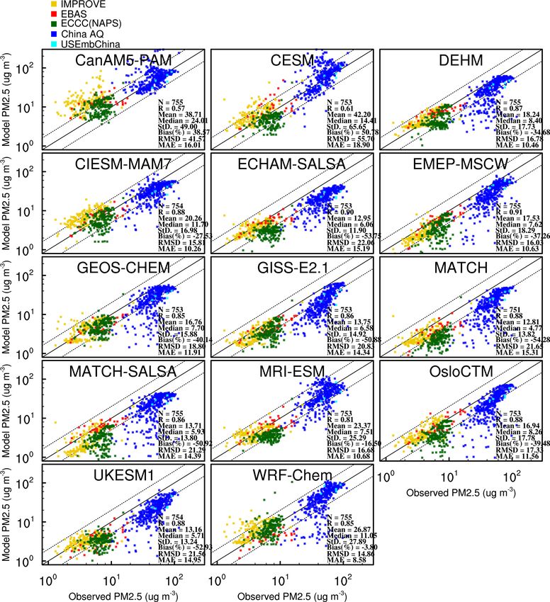
5782                                                                             C. H. Whaley et al.: AMAP SLCF model evaluation

Figure 1. Locations of Arctic surface in situ measurements, including (a) O3 , (b) BC in brown, and ice cores in black, as well as (c) SO2−
                                                                                                                                         4 .

   Organic carbon (OC) is also measured via thermal and/or              ACT2: McConnell and Edwards, 2008; Humboldt: Bauer
thermal–optical methods (Chow et al., 1993, 2001, 2004;                 et al., 2013; Summit: Maselli et al., 2017; NGT_B19,
Huang et al., 2006; Cavalli et al., 2010; Chan et al., 2019;            ACT11D: McConnell et al., 2019). The Arctic SO2−
                                                                                                                      4 mea-
Huang et al., 2021) using the same instrumentation as for EC            surement locations are shown in Fig. 1.
detection in IMPROVE, CABM, NAPS, and EMEP measure-
ment networks. These OC measurements have approximately                 3.1.5    PM2.5
20 % or less uncertainty (Chan et al., 2019). Models output
organic aerosol (OA), which includes OC and organic mat-                Surface in situ PM2.5 measurements are usually made via
ter and is related to OC via a factor of 1.4 (Russell, 2003;            gravimetric analysis of particulate matter collected on a filter
Tsigaridis et al., 2014), though this factor has been reported          (e.g., Teflon substrate), which has around a 1 %–6 % uncer-
as a range from 1.4 to 2.1 in the literature, depending on the          tainty range (Malm et al., 2011). These data were obtained
source of OC and OA (Tsigaridis et al., 2014). Nevertheless,            from Beijing Air Quality and US Embassy data for China,
we applied a conversion factor of 1.4 to the OC measure-                NAPS for Canada (Dabek-Zlotorzynska et al., 2011), IMR-
ments before comparing the modeled OA.                                  PROVE for the US, and EMEP and/or EBAS for Europe.
   Arctic BC measurement locations are shown in Fig. 1, and
many of these Arctic aerosol measurements were discussed                3.2     Satellite datasets
in Schmale et al. (2022). We also evaluated modeled BC de-
                                                                        Satellite observations are useful for evaluating models on
position by comparing it to BC deposition derived from ice
                                                                        larger horizontal spatial scales and for evaluating the three-
core measurements (D4, ACT2: McConnell and Edwards,
                                                                        dimensional atmosphere – not the surface concentrations.
2008; Humboldt: Bauer et al., 2013; Summit: Keegan et al.,
                                                                        Observations from three satellite instruments were used to
2014; NGT_B19, ACT11D: McConnell et al., 2019). All of
                                                                        evaluate model trace gas distributions in the free troposphere
the ice core locations are also shown in Fig. 1. Deposition
                                                                        and, when appropriate, the lower stratosphere. These were
fluxes are not a measured value but are derived from the EC
                                                                        the Tropospheric Emission Spectrometer version 7 (TES;
concentrations in ice and precipitation estimates.
                                                                        NASA Atmospheric Science Data Centre, 2018; Gluck,
                                                                        2004a, b), the Atmospheric Chemistry Experiment–Fourier
3.1.4   SO2−
          4
                                                                        Transform Spectrometer version 4.1 (ACE-FTS; Bernath
                                                                        et al., 2005; Sheese and Walker, 2020), and the Measure-
Surface in situ SO2−
                  4 measurements in the major observing                 ments of Pollution in the Troposphere version 8 (MOPITT;
networks typically use ion chromatography methods, which                Ziskin, 2000; Deeter et al., 2019). The vertical profiles of
have an approximately 3 % uncertainty range (Solomon                    trace gas volume mixing ratios are derived or retrieved from
et al., 2014). However, SO2− 4   measurements have been                 the satellite-measured emission or absorption spectra, with
shown to have up to 20 % analytical uncertainty (AMAP,                  varying degrees of vertical sensitivity. These remote tech-
2022). SO2−
          4 datasets were obtained from IMPROVE, EMEP,                  niques typically have about a 15 % uncertainty in the mea-
and CABM networks, often via the EBAS database.                         surements (e.g., Verstraeten et al., 2013), though this depends
  SO2−4  deposition was also derived from the same ice                  on the specific instrument and the species retrieved (e.g.,
core measurements mentioned above for BC deposition (D4,                Sheese et al., 2017).

Atmos. Chem. Phys., 22, 5775–5828, 2022                                                    https://doi.org/10.5194/acp-22-5775-2022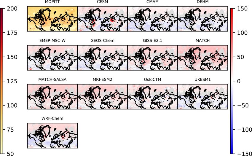
C. H. Whaley et al.: AMAP SLCF model evaluation                                                                                 5783

   Note that while TES and MOPITT have global spatial cov-
erage, their coverage does not extend up into the high Arc-
tic. The TES instrument on NASA’s Aura satellite measures
vertical profiles of trace gases such as O3 , CH4 , NO2 , CO,
and HNO−     3 from 2004–present. After interpolating all mod-
els and TES results to a 1◦ × 1◦ horizontal grid, the monthly
mean CH4 and O3 from the TES lite products were matched
in space and time with models. Models were smoothed with
the TES monthly mean averaging kernels prior to compar-
isons with satellite data. TES measurements started in 2004,
stopped in late 2015, and had poorer coverage in the last few
years.
   A similar comparison method was used for MOPITT data.
The MOPITT instrument on NASA’s Terra satellite measures
CO from 2000 to the present.
   The ACE-FTS instrument on CSA’s SCISAT satellite has
measured the trace gases O3 , CO, NO, NO2 , and CH4 ,
among over 30 others from 2004–present. SCISAT has a
high-inclination orbit, giving its instruments better coverage
in the Arctic. ACE-FTS is a limb-sounding instrument mea-
suring the solar absorption spectra of dozens of trace gas con-
centrations from the upper troposphere to the thermosphere.       Figure 2. Flight tracks of BC aircraft campaigns used in this study.
This gives us the opportunity to evaluate the 3-D model out-
put in a region of the atmosphere where the radiative forcing
of ozone is at its highest. Evaluating models with ACE-FTS        3.3.1   Aircraft campaigns
measurements also provides insight into models’ transport
and upper-tropospheric chemistry. As was shown in Kolon-          The flight paths of the aircraft used for model evaluation of
jari et al. (2018), 3-hourly model output (rather than monthly    BC are shown in Fig. 2. The aircraft campaigns include A-
mean output) is required for accurate comparisons to ACE-         FORCE (Oshima et al., 2012), ARCPAC (Brock et al., 2011),
FTS data; thus, only models that provided output at this time     ARCTAS (Jacob et al., 2010), EUCAARI (Hamburger et al.,
frequency were compared to ACE-FTS measurements. The              2011), HIPPO (Schwarz et al., 2010), NETCARE (Schulz
model output was sampled to match the times and locations         et al., 2019), and PAMARCMIP (Stone et al., 2010). Most of
of ACE-FTS measurements. We used an updated version of            these aircraft campaigns occurred during boreal spring and
the advanced method in Kolonjari et al. (2018). Instead of        summer months (April to July) except for one (HIPPO) oc-
taking the model output at the closest time to the ACE-FTS        curring in January and November, and most occurred during
measurement time, the model output was linearly interpo-          the 2008–2009 time period, with only one (NETCARE) oc-
lated onto the ACE-FTS time. This reduces the bias intro-         curring during 2014–2015. All of these aircraft campaigns
duced by diurnal cycles, which can cause certain volume           measured rBC from single-particle soot photometers (SP2)
mixing ratios (VMRs; e.g., that of NO and NO2 ) to vary sig-      (Moteki and Kondo, 2010; Schwarz et al., 2006; Stephens
nificantly between model output times. As in Kolonjari et al.     et al., 2003).
(2018), the model output is also interpolated vertically in log      The AMAP models that submitted 3-hourly BC output
pressure space and bilinearly in latitude and longitude to ac-    were linearly interpolated onto the aircraft locations in space
count for spatial variation between model grid points.            and time using the Community Intercomparison Suite (CIS;
                                                                  Watson-Parris et al., 2016) in order to provide representative
                                                                  comparisons and robust evaluation.
3.3   Measurement campaigns
Finally, there were air- and ship-based measurement cam-
                                                                  3.3.2   Ship campaigns
paigns of black carbon that were used for model evalua-
tion. Aircraft campaigns allow vertical profiles of chemical      There were three ship-based measurement campaigns in
species to be evaluated, and ship campaigns allow for in situ     2014–2015. These were the two Japanese campaigns (MR14-
measurements in the remote Arctic seas.                           05 and MR15-03 cruises of R/V Mirai) in September of
                                                                  2014 and 2015 (track from Japan to north of Alaska; Take-
                                                                  tani et al., 2016) and the Russian campaign in October
                                                                  2015 (track north of Russia, from Arkhangelsk to Severnaya
                                                                  Zemlya and back; Popovicheva et al., 2017) – both are shown

https://doi.org/10.5194/acp-22-5775-2022                                           Atmos. Chem. Phys., 22, 5775–5828, 2022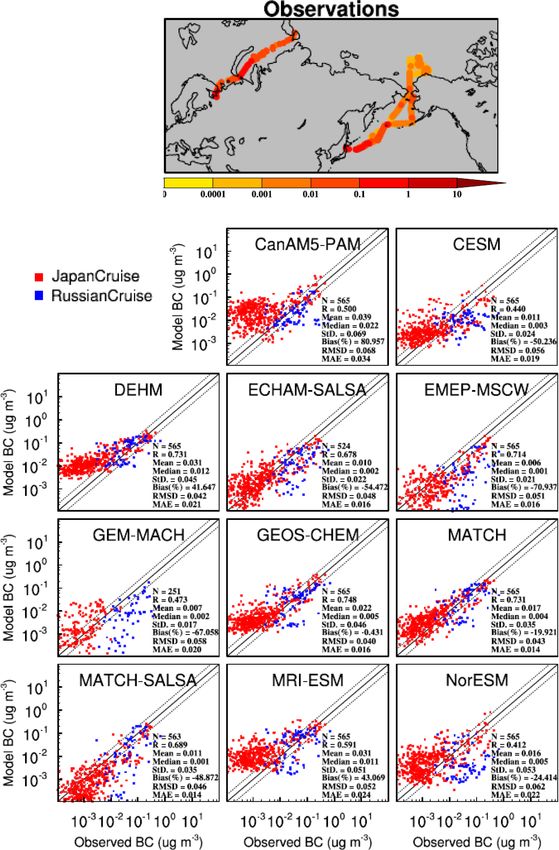
5784                                                                       C. H. Whaley et al.: AMAP SLCF model evaluation

in Sect. 4.5 (Fig. 17). Models that provided 3-hourly BC out-      mmm bias was high at the midlatitudes, it is close to zero in
put were compared to these observations. The Russian mea-          the Arctic (O3 ), and if the mmm bias was near zero at mid-
surements of aerosol eBC concentrations were determined            latitudes, it is negative in the Arctic (NO2 , BC, SO2−4 ). This
continuously using an Aethalometer purposely designed by           implies that there is not enough long-range transport from the
MSU/CAO (Popovicheva et al., 2017). Light attenuation              midlatitude source regions to the Arctic. That said, the mmm
caused by the particles depositing on a quartz fiber filter was    CH4 bias stays relatively constant with latitude, and we will
measured, and the light attenuation coefficient of the col-        see in Sect. 4.2 that this result is model-dependent. The CO,
lected aerosol was calculated. eBC concentrations were de-         PM2.5 , and OA mmm biases have an increasing trend with
termined continuously by converting the time-resolved light        latitude. However, both CO and PM2.5 have no observation
attenuation to the eBC mass corresponding to the same atten-       locations in the high Arctic, so those results cannot represent
uation and characterized by a specific mean mass attenuation       long-range transport. OA only has one observation location
coefficient, in calibration with AE33 (Magee Scientific).          in the high Arctic, and its bias is very large overall, so issues
   The Japanese measurements provide rBC (refractory BC).          other than long-range transport are at play, as we will see in
Pileci et al. (2021) showed that rBC and eBC are lin-              the following discussion (Sect. 4.7).
early related; thus, in order to compare the observations             Of course, there are spatial, temporal, and model differ-
to models, we converted rBC to eBC via a factor of 1.8             ences in the results, so we will now explore model perfor-
(eBC = 1.8 × rBC; Zanatta et al., 2018; Pileci et al., 2021).      mance for each SLCF in more detail in the next subsections.

4     Model–measurement comparisons                                4.2   Methane

In this section, we evaluate modeled SLCFs from the 18 par-        Measured annual mean surface methane is shown in the top
ticipating models with a focus on performance in the North-        left panel of Fig. 5, along with model biases in the rest of the
ern Hemisphere midlatitudes (defined for our purposes as           panels. Recall that unlike the rest of the SLCF species in this
30–60◦ N) and the Arctic (defined here as > 60◦ N for sim-         study, CH4 concentrations were prescribed in these models
plicity). Unless otherwise noted, the observations are com-        from the same CH4 dataset (Olivié et al., 2021). That said,
pared to the model grid box that they are located in, and          the different decisions by modelers on how those CH4 global
when more than one observation location occurs in the same         concentrations are distributed make differences in how these
model grid box, those observations are averaged first before       models compare to measurements. The mean model biases
the comparison. We look at spatial patterns in the model bi-       are small and mainly positive; in the midlatitudes, the multi-
ases, as well as the vertical distribution and the seasonal cy-    model mean bias is +145 ppbv (or +8.5 %), and in the Arc-
cles for each species, but first we start by providing a multi-    tic, the mmm bias is 24 ppbv (or 1.3 %), which means that the
species summary of the annual mean model biases in the sur-        models simulate the magnitude of surface CH4 well – though
face air.                                                          still outside the < 1 % measurement uncertainty range. There
                                                                   is a gradient in CH4 VMRs (higher in the Northern Hemi-
                                                                   sphere and lower in the Southern Hemisphere) that is seen
4.1    Multi-species summary
                                                                   in the measurements (Fig. 5, top left) and reported in the
The 2014–2015 average modeled percent biases for surface           literature (e.g., Dlugokencky et al., 1994), though it is not
concentrations of SLCFs are shown in Fig. 3 for each model         well captured by CMAM, MRI-ESM2, and UKESM1 mod-
and the multi-model mean (mmm). This figure is based on            els, which are all biased low in the Northern Hemisphere and
the model comparisons at the surface observation locations         biased higher towards the south. That is because of the sim-
that will be shown in subsequent sections (Figs. 1, 5, 7, 10,      plifications made in these models’ distributions of CH4 . For
11, 13, 18, 21, and 23 and additional American observations        example, CMAM used a single global average CH4 concen-
from the IMPROVE network for BC, SO2−      4 , and OA).            tration that is interpolated linearly in time from once-yearly
   Figure 3b shows that, for surface Arctic concentrations,        values.
no one model performs best for all species but that the mmm           Figure 5 also shows that observed annual mean surface
performs particularly well. It also shows that the model bi-       CH4 ranges geographically from about 1500 to 2100 ppbv
ases vary quite a bit among SLCF species for both the mid-         depending on location; however, the models have a much
latitudes and the Arctic. It is important to note that there are   smaller range due to their prescribing CH4 concentrations as
many more measurement locations at midlatitudes compared           a lower boundary input. For example CMAM CH4 volume
to in the Arctic. BC, CH4 , O3 , and PM2.5 have the smallest       mixing ratios only span about ±3 ppbv around 1836 ppbv.
model biases out of the SLCFs of this study, whereas OA,           The span of MRI-ESM2 surface CH4 is even smaller. GEOS-
CO, and NO2 have larger model biases.                              Chem, GISS-E2.1, and OsloCTM have a more realistic range
   We find for half of the SLCF species that the mmm percent       of 1700–2000 ppbv, though they still do not get the full vari-
bias decreases with latitude (Fig. 4). O3 , NO2 , BC, and SO4      ability that is seen in surface CH4 mixing ratios close to
have a negative slope in the bias vs. latitude figure. So if the   CH4 sources. However, in the free troposphere (above the

Atmos. Chem. Phys., 22, 5775–5828, 2022                                              https://doi.org/10.5194/acp-22-5775-2022
C. H. Whaley et al.: AMAP SLCF model evaluation 5785
Figure 3. Mean 2014–2015 model percent biases for each model and the mmm for surface SLCF concentrations as well as BC and SO2−
4
deposition at (a) midlatitudes and (b) the Arctic. Note that the color scale is not linear.
models’ simulations to ozonesonde measurements and in our
satellite O3 comparison in the next section. The CH4 model–
measurement correlation coefficients for ACE-FTS are rela-
tively high (e.g., R = 0.48 to 0.86 depending on the model).
Therefore, the general model evaluation for CH4 indicates
that because models do not explicitly model CH4 emissions,
they do not simulate the surface-level variability of CH4
VMRs. Models differ in their global distribution of CH4 ;
thus, only some contain the north–south CH4 gradient. Those
that do not have the largest underestimations of Arctic tropo-
spheric CH4 . The CH4 evaluation also implies that the mod-
eled tropopause height may be too low.
Figure 4. Multi-model mean percent biases for surface SLCF con-
centrations versus latitude (in 10◦ latitude bins).
4.3 Ozone
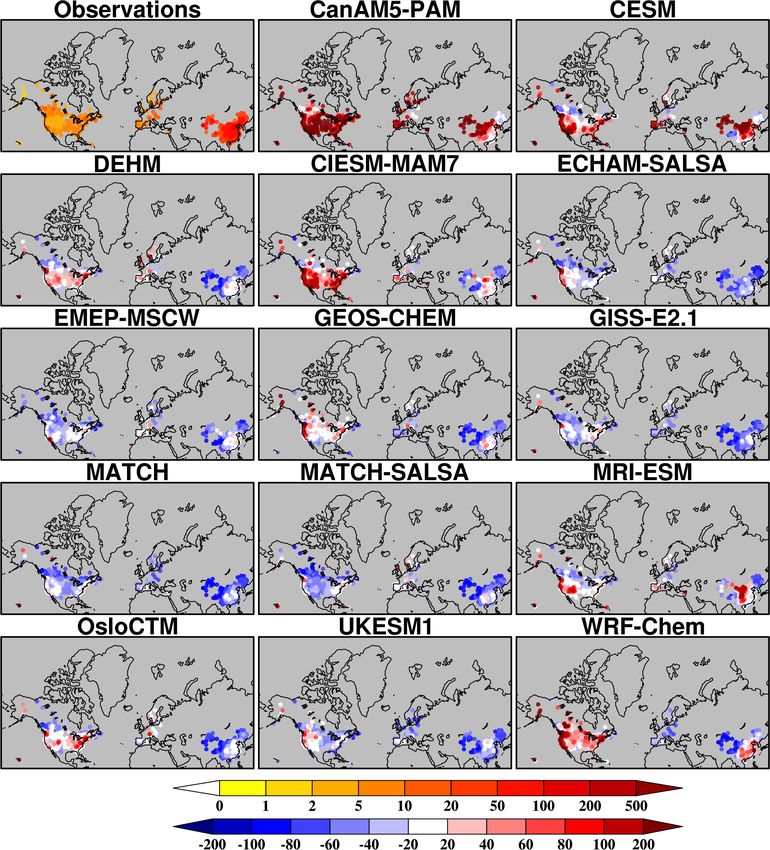
boundary layer), we have TES satellite measurements of Tropospheric O3 is the third most important greenhouse gas
CH4 that show that CH4 is much more smoothly distributed (IPCC, 2021), and it is a regional pollutant that causes dam-
aloft. Thus, the simplification of prescribing CH4 concen- age to human health and ecosystems. O3 is a secondary pol-
trations in the models is more realistic there (Fig. 6, show- lutant formed in the troposphere via photochemical oxidation
ing the 600 hPa level in the mid-troposphere). Additionally, of volatile organic compounds in the presence of nitrogen
Fig. 6 better illustrates the latitudinal gradient in CH4 over oxides (NOx = NO + NO2 ). As such, models must simul-
the globe and its lack in some models, which have more neg- taneously simulate the meteorological conditions, precursor
ative biases in the Northern Hemisphere and more positive species distributions, and photochemistry correctly in order
biases in the Southern Hemisphere. Other models, such as to accurately simulate O3 . That said, since surface O3 is an
GISS-E2.1, do a good job of capturing the global distribu- important contributor to poor air quality, there is significant
tion of CH4 . pressure for models to simulate it accurately, particularly in
In the Arctic, the vertical cross section of CH4 VMRs over the heavily populated midlatitudes (e.g., for air quality fore-
time as measured by the ACE-FTS in the middle to upper tro- casting). Only models with prognostic O3 are included in this
posphere and in the stratosphere is shown in Fig. S1. There is section.
a large decrease in CH4 above the tropopause at around 300– Figure 7 shows the in situ summertime mean O3 measure-
100 hPa. The models are all biased low around 300 hPa and ments (top left panel), and the model biases (remaining pan-
high around 100 hPa. This pattern is true for midlatitudes as els) and the same for the annual mean is shown in the Sup-
well as in the Arctic and may imply that the altitude of the plement (Fig. S2). These include averaging O3 from hourly
modeled tropopause is too low. This same conclusion was observations (day and night) and 3-hourly or monthly mod-
also found in Whaley et al. (2022a) via comparisons of these eled O3 depending on which were available for each model.
https://doi.org/10.5194/acp-22-5775-2022 Atmos. Chem. Phys., 22, 5775–5828, 20225786 C. H. Whaley et al.: AMAP SLCF model evaluation Figure 5. Measured surface-level methane (top left) (ppbv, left color bar) and (remaining panels) model biases (model minus measurement, also ppbv, right color bar) for 2014–2015. Figure 6. TES measurements (top left) of CH4 in the mid-troposphere (at 600 hPa, ppbv, left color bar) and (remaining panels) model biases for 2008–2009 (model minus measurement, also ppbv, right color bar). Results for 2014–2015 are similar but had less spatial coverage by the satellite. Gray areas have no data (either from the model, TES, or both). Surface O3 is overpredicted by most models, which has mean has a bias of +11 % for the Arctic, but this is not uni- been documented previously (Makar et al., 2017; Turnock formly spatially distributed. All models overestimated sur- et al., 2020). It has been shown that models can have prob- face O3 in Alaska (mainly due to the overestimation of sum- lems producing low O3 overnight (Brown et al., 2006; Lin mertime concentrations, discussed below), and most models et al., 2008). In the Arctic, simulated surface O3 has more have too little O3 at the Greenland location and in northern mixed results. Annual mean concentrations are of the order Europe. of 40 ppbv, and individual model biases range from −20 % to +52 % globally on average for 2014–2015. The multi-model Atmos. Chem. Phys., 22, 5775–5828, 2022 https://doi.org/10.5194/acp-22-5775-2022
C. H. Whaley et al.: AMAP SLCF model evaluation                                                                                    5787

Figure 7. Summertime (JJA) (top left) mean in situ surface O3 measurements (ppbv, left color bar) and (remaining panels) model biases for
2014–2015 (model minus measurement, also ppbv, right color bar). Results for 2008–2009 are similar but are not available for China.

   The models were all able to represent the summertime                gen chemistry (Bottenheim et al., 1986; Barrie et al., 1988;
peak in the midlatitude seasonal cycle (not shown). In con-            Simpson et al., 2007). None of the model simulations in this
trast to the more polluted midlatitudes, where surface O3              study contain the necessary tropospheric halogen chemistry
peaks in the summertime due to photochemical production                to simulate those events, which partly explains why some
being at a maximum, Arctic O3 is more influenced by the                models in Fig. 8 (bottom) overestimate springtime O3 con-
Brewer–Dobson circulation, bringing a maximum of tropo-                centrations. That particular feature is explored further on a
spheric O3 in the springtime due to photochemical produc-              site-to-site basis in Whaley et al. (2022a).
tion (Wespes et al., 2012), descent from the stratosphere,                The next subsection shows that both the O3 precursors CO
and more long-range transport of O3 to the Arctic. Fig-                and NO2 are underestimated compared to measurements at
ure 8, shows this springtime peak in both the western (a,              all global locations. This has implications for simulated tro-
longitude < 0◦ ) and eastern (b, longitude > 0◦ ) Arctic in the        pospheric O3 chemistry.
measurements. However, the models only capture that sea-                  Free-tropospheric O3 – satellite comparisons. Aircraft-
sonal cycle in the eastern Arctic (Fig. 8b), implying that the         based measurements and ozonesondes can provide insight
models represent large-scale circulation and possibly strato-          into the vertical distribution of O3 , and these have been
sphere to troposphere exchange well. But it is interesting to          well documented (e.g., Tarasick et al., 2019; Whaley et al.,
note that the models that have sophisticated representation of         2022a). However, model grid boxes may not be representa-
stratosphere–troposphere exchange (such as CMAM, MRI-                  tive of those fine-spatial-scale measurements. In this study,
ESM2, UKESM1) do not particularly stand out as better per-             we examine how the model biases change in the vertical
formers in Fig. 8 compared to models that do not simulate the          when compared to satellite measurements, which have a
stratosphere (such as DEHM, MATCH, MATCH-SALSA).                       larger, “smoothed out” spatial sensitivity due to their view-
Thus, its impact on surface O3 may be very small.                      ing geometry and retrieval methods. Specifically, we com-
   In the western Arctic (Alaska mainly, Fig. 8a), models              pare modeled O3 to TES and ACE-FTS satellite-based re-
overestimate summertime Arctic O3 , likely due to overpre-             trievals. These satellite instruments also have better global
dicting the impact of wildfire emissions on tropospheric O3            coverage than aircraft and sonde-based measurements.
concentrations, which is a research topic with high uncer-                The model fractional biases compared to TES measure-
tainty (van der Werf et al., 2010; Monks et al., 2015; Arnold          ments from near the surface up to 100 hPa are shown in Fig. 9
et al., 2015). Another possibility is that modeled O3 dry de-          for the Arctic (left) and midlatitudes (right). All models’
position over boreal vegetation is underestimated (Stjernberg          simulated fractional biases have similar vertical profiles for
et al., 2012; Thorp et al., 2021).                                     both the Arctic and midlatitudes, with greater negative val-
   Some Arctic locations are more inclined to get springtime           ues at lower levels and a more positive “bulge” of about 10 %
surface O3 depletion due to bromine explosions and halo-               around 300 hPa in the Arctic and about 5 % around 200 hPa

https://doi.org/10.5194/acp-22-5775-2022                                               Atmos. Chem. Phys., 22, 5775–5828, 2022
5788                                                                         C. H. Whaley et al.: AMAP SLCF model evaluation

Figure 8. Surface O3 monthly range that occurs at the locations in Fig. 7 above 60◦ N. The measurements are the black and white boxes
and whiskers, and the models are the colored box and whiskers. (a) The western Arctic and (b) the eastern Arctic for 2014–2015. Thick
horizontal lines indicate the median O3 VMR in each month, and the box extends to the interquartile range. The whiskers extend to the
minimum and maximum monthly mean O3 VMR.

at midlatitudes. That bulge in model biases at 300 hPa was           tic region and in lower troposphere in the midlatitude region,
also seen to a greater degree (50 %–70 %) when comparing             whereas a positive bias is seen in the upper troposphere be-
these model simulations to Arctic ozonesonde measurements            low 60◦ N. This is consistent for the two time periods (2008–
in Whaley et al. (2022a). Compared to TES, which has much            2009 and 2014–2015).
lower vertical resolution, the results are not as striking but          Given that Fig. 7 shows positive biases near the midlati-
are consistent with ACE-FTS measurements. On average, the            tudes, while Fig. 9 shows lower O3 in the free troposphere,
models have a negative bias at all vertical levels in the Arc-       these results imply that there is not enough vertical lifting

Atmos. Chem. Phys., 22, 5775–5828, 2022                                               https://doi.org/10.5194/acp-22-5775-2022
C. H. Whaley et al.: AMAP SLCF model evaluation                                                                                   5789

Figure 9. Vertical distribution of models’ O3 percent biases (model minus measurement over measurement) for 2008–2009 compared to the
TES measurements; (a) average for midlatitudes (30–60◦ N) and (b) average for Arctic latitudes (> 60◦ N).

and/or mixing of tropospheric O3 in most of the models.
However, the TES measurements have been shown to be
biased high by approximately 13 % throughout the tropo-
sphere (Verstraeten et al., 2013), which is the same amount
that the mmm is low. Similarly, ACE-FTS O3 has an uncer-
tainty range of +5 %–10 % when compared to O3 from other
satellite limb-view observations (Sheese et al., 2017). The
ACE-FTS comparison for O3 can be found in the Supplement
(Fig. S3), showing higher model biases around 300–100 hPa
(except for GEOS-Chem) and good agreement below that.
Therefore, overall, participating models simulate the free-
tropospheric O3 reasonably well and within the uncertainly
limits of the observations.
   Therefore, the general model evaluation for O3 indicates            Figure 10. Mean CO volume mixing ratios (ppbv, left color bar) at
that all models overestimate surface O3 at midlatitudes, and           surface measurement sites and MMM bias (MMM minus measure-
that, combined with a lack of O3 transport to the Arctic, re-          ment ppbv, right color bar) for 2014–2015. Results from 2008–2009
sults in modeled Arctic O3 VMRs having relatively little bias          are similar and not shown.
(the right answer for the wrong reason). The summertime
evaluation implies that models overestimate the O3 produced
and transported by wildfires in the western Arctic. The O3             mons et al., 2015; Monks et al., 2015; Jiang et al., 2015;
evaluation also implies that the modeled tropopause height             Quennehen et al., 2016), pointing to a likely underestimation
may be too low.                                                        of CO emissions and possibly shorter modeled lifetimes of
                                                                       CO due to an overestimation in OH (Miyazaki et al., 2012).
4.4   O3 precursors: carbon monoxide and nitrogen                      The annual mean surface CO underestimation is mainly dom-
      oxides                                                           inated by the wintertime (e.g., the mmm bias in DJF is
                                                                       −92 %), when it has been reported that CO emissions from
Figures 10 and 11 show the comparisons of the multi-model              combustion are too low (e.g., Kasibhatla et al., 2002; Pétron
medians (MMMs) to the surface in situ measurements. The                et al., 2002). All the models exhibit a large negative bias over
figures for each model appear in the Supplement (Figs. S4              China, which is consistent with the study by Quennehen et al.
and S5), but only the MMMs are shown here since the spatial            (2016) and is attributed to the enhanced destruction of CO by
patterns were very similar for all models. The multi-model             OH radicals, but it was also found in Kasibhatla et al. (2002)
annual mean underpredicts both CO and NO2 by approxi-                  and Pétron et al. (2002) that bottom-up CO emission inven-
mately −55 % in the Northern Hemisphere for 2014–2015.                 tories in Asia are greatly underestimated.
The 2015 AMAP report showed similar findings for simu-                    In the free troposphere, we compare modeled CO to that
lated surface CO, as have other studies (AMAP, 2015a; Em-              measured by MOPITT. Figure 12 shows these comparisons

https://doi.org/10.5194/acp-22-5775-2022                                               Atmos. Chem. Phys., 22, 5775–5828, 2022
You can also read