MIXED PROBABILITY MODELS FOR ALEATORIC UNCERTAINTY ESTIMATION IN THE CONTEXT OF DENSE STEREO MATCHING
←
→
Page content transcription
If your browser does not render page correctly, please read the page content below
ISPRS Annals of the Photogrammetry, Remote Sensing and Spatial Information Sciences, Volume V-2-2021
                                              XXIV ISPRS Congress (2021 edition)

    MIXED PROBABILITY MODELS FOR ALEATORIC UNCERTAINTY ESTIMATION IN
                 THE CONTEXT OF DENSE STEREO MATCHING

                                                    Zeyun Zhong∗, Max Mehltretter

                       Institute of Photogrammetry and GeoInformation, Leibniz University Hannover, Germany
                                            (zeyun.zhong, mehltretter)@ipi.uni-hannover.de

                                                       Commission II, WG II/2

KEY WORDS: Uncertainty Quantification, 3D Reconstruction, Deep Learning, Mixture Model

ABSTRACT:

The ability to identify erroneous depth estimates is of fundamental interest. Information regarding the aleatoric uncertainty of depth
estimates can be, for example, used to support the process of depth reconstruction itself. Consequently, various methods for the
estimation of aleatoric uncertainty in the context of dense stereo matching have been presented in recent years, with deep learning-
based approaches being particularly popular. Among these deep learning-based methods, probabilistic strategies are increasingly
attracting interest, because the estimated uncertainty can be quantified in pixels or in metric units due to the consideration of
real error distributions. However, existing probabilistic methods usually assume a unimodal distribution to describe the error
distribution while simply neglecting cases in real-world scenarios that could violate this assumption. To overcome this limitation, we
propose two novel mixed probability models consisting of Laplacian and Uniform distributions for the task of aleatoric uncertainty
estimation. In this way, we explicitly address commonly challenging regions in the context of dense stereo matching and outlier
measurements, respectively. To allow a fair comparison, we adapt a common neural network architecture to investigate the effects
of the different uncertainty models. In an extensive evaluation using two datasets and two common dense stereo matching methods,
the proposed methods demonstrate state-of-the-art accuracy.

                      1. INTRODUCTION                                  pixel’s depth estimate and can be learned as a binary class prob-
                                                                       ability of a depth estimate being correct or incorrect (Hu and
Depth estimation from images, i.e., reconstructing the per-pixel       Mordohai, 2012). In contrast, probabilistic methods assume a
distance between a scene and a camera, is a classical task in          certain probability distribution for aleatoric uncertainty which
photogrammetry as well as in computer vision. It has many ap-          is optimised during training maximising the likelihood (Kend-
plications in practice, including fields of autonomous vehicles        all and Gal, 2017). While this approach requires more detailed
and UAVs. It also serves as a foundation to support other photo-       knowledge on the real error distribution, contrary to the concept
grammetric computer vision problems, such as 3D reconstruc-            of confidence-based methods, it allows to additionally quantify
tion and object detection. As a central step of depth estima-          the uncertainty in pixels or in metric units. These probabilistic
tion in any photogrammetric 3D reconstruction, the core task of        methods usually assume a unimodal distribution, considering
dense stereo matching is the determination of pixel correspond-        the error distribution as a Gaussian (Kendall and Gal, 2017) or
ences for all pixels in an image pair. It is challenging to achieve    a Laplacian distribution (Mehltretter and Heipke, 2021). How-
this objective robustly in real-world scenarios due to a variety of    ever, this is not always the case in the context of dense stereo
problems, such as occlusions, thin structures and large weakly         matching and does especially not account for outlier measure-
textured areas, e.g. in the sky or caused by over-exposure. Con-       ments or commonly challenging regions, such as texture-less
sequently, the accuracy of the estimated depth information may         regions, occlusions and depth discontinuities.
be affected, making it crucial to be able to assess how trust-         To overcome these limitations, we propose two novel mixed
worthy this information is.                                            probability models for aleatoric uncertainty estimation, using
                                                                       different combinations of a Laplacian and a Uniform distribu-
To address the task of uncertainty quantification in the context       tions under varying assumptions. We evaluate our proposed
of dense stereo matching, in this work, we focus on the estim-         methods together with the state-of-the-art probabilistic aleatoric
ation of aleatoric uncertainty. From the perspective of dense          uncertainty model, i.e., Laplacian model, on two different data-
stereo matching, aleatoric uncertainty accounts for effects such       sets, containing outdoor and indoor scenes, respectively. For
as sensor noise, occlusion, depth discontinuities and match-           a fair comparison, the Cost Volume Analysis Network (CVA-
ing ambiguities caused by texture-less areas or repetitive pat-        Net) (Mehltretter and Heipke, 2021) is adapted to investigate
terns (Mehltretter and Heipke, 2021). In the literature, a variety     the differences and effects of these three uncertainty models.
of different deep learning-based approaches to estimate aleat-         Thus, the main contributions of this work are:
oric uncertainty have been proposed in recent years demonstrat-
ing convincing results. Among them, two types of strategies are          • A geometry-aware probabilistic aleatoric uncertainty
especially popular: confidence-based and probabilistic-based.              model that explicitly models regions that are challenging
Confidence-based methods predict a score between zero and                  in the context of dense stereo matching.
one for each pixel, which indicates the trust that is put in a
                                                                         • A mixture probabilistic aleatoric uncertainty model expli-
∗   Corresponding author                                                   citly considering outlier measurements.

           This contribution has been peer-reviewed. The double-blind peer-review was conducted on the basis of the full paper.
                       https://doi.org/10.5194/isprs-annals-V-2-2021-17-2021 | © Author(s) 2021. CC BY 4.0 License.                   17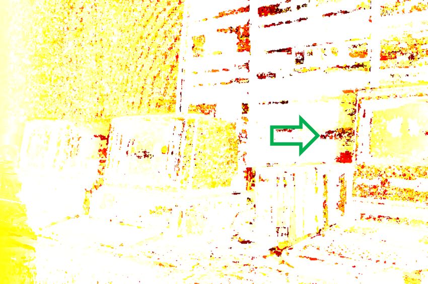
ISPRS Annals of the Photogrammetry, Remote Sensing and Spatial Information Sciences, Volume V-2-2021
                                             XXIV ISPRS Congress (2021 edition)

  • An adaption of the CVA-Net architecture for the proposed          this assumption is violated by outlier measurements or by com-
    uncertainty models. In addition, the network architecture         monly challenging regions, such as occlusion, texture-less re-
    is optimised to accelerate the training procedure.                gions and depth discontinuities. Simply neglecting these cases
                                                                      leads to an over-simplification that may reduce the accuracy of
                                                                      the estimated aleatoric uncertainty.
                    2. RELATED WORK

As the ability to reliably detect failures of a stereo algorithm                          3. METHODOLOGY
is fundamental, many approaches have been proposed in re-
cent years to estimate the uncertainty of disparity assignments.      To adjust the probabilistic strategy of aleatoric uncertainty es-
At first, hand-crafted metrics were designed to quantify aleat-       timation in the context of dense stereo matching to better fit
oric uncertainty, such as Peak Ratio (PKR), which is designed         to the characteristics of real-world scenarios, we propose two
based on the properties of the cost curve, and Left Right Dif-        novel uncertainty models based on two different assumptions,
ference (LRD), which considers the consistency between the            which are discussed in detail in Section 3.2. For the purpose
left and the right disparity maps. A good overview of the com-        of a fair comparison of different uncertainty models, i.e. avoid-
monly used hand-crafted metrics is given in (Hu and Mordohai,         ing the impacts coming from the disparity estimation process or
2012). Similar to other computer vision fields, more and more         different network architectures used to carry out the task of un-
approaches based on deep learning (Poggi and Mattoccia, 2016;         certainty prediction, we test all variants using the same neural
Mehltretter and Heipke, 2019; Kendall and Gal, 2017) and other        network architecture, which focuses only on the uncertainty es-
machine learning techniques (Sun et al., 2017; Batsos et al.,         timation process. In detail, this architecture (briefly outlined in
2018) have been proposed in the literature. While a majority          Section 3.1) utilises cost volumes as input, which are the result
of these deep learning-based uncertainty estimation methods,          of the cost computation step of an arbitrary dense stereo match-
operate on extracted patches from disparity maps only (Poggi          ing approach carried out on an epipolar rectified image pair.
and Mattoccia, 2016) or additionally take the RGB reference
                                                                      3.1   Basic Architecture
image into account (Fu et al., 2019), Mehltretter and Heipke
(2019) utilise the information contained in the 3D cost volume.       Showing convincing results for the task of aleatoric uncertainty
Such a cost volume is an intermediate representation present in       estimation in (Mehltretter and Heipke, 2019, 2021), the archi-
most dense stereo matching algorithms which typically contains        tecture of the Cost Volume Analysis Network (CVA-Net) is util-
additional information compared to disparity maps. Benefiting         ised to evaluate our subsequently proposed probabilistic uncer-
from this additional information, cost volume-based approaches        tainty models. This network consists of three major processing
have demonstrated to allow a more accurate estimation of the          steps: First, a three-dimensional cost volume extract is merged
uncertainty.                                                          to a single 1D feature vector, using 3D convolutional layers.
                                                                      To keep a good trade-off between the amount of information
While plenty of literature exists focusing on various types of
                                                                      available to the network and the degree of smoothing within the
features, modelling the aleatoric uncertainty has received sig-
                                                                      resulting uncertainty map, we follow (Mehltretter and Heipke,
nificantly less attention. Among these uncertainty estimation
                                                                      2021), setting the size of such extract to 13×13×192. In the
methods, the confidence-based strategy is most popular (Fu et
                                                                      second step, the resulting 1D feature vector is further processed
al., 2019; Tosi et al., 2018). Driven by the fact that, in contrast
                                                                      using 3D convolutional layers to derive high-level features char-
to depth, ground truth is typically not available for the asso-
                                                                      acterising the cost volume extract. Based on the extracted fea-
ciated uncertainty in the form of the type and parameters of a
                                                                      tures, two fully-connected layers, which are implemented in a
particular distribution, uncertainty prediction has to be learned
                                                                      convolutional manner, are then utilised to predict an uncertainty
implicitly by assuming a specific uncertainty model. For this
                                                                      value in the last step.
purpose, confidence-based methods predict a score per pixel
between zero and one, representing the trust on the correspond-       While CVA-Net demonstrates convincing results, the usage of
ing depth estimate, and thus, can be learned as a binary class        3D instead of 2D convolutional layers leads to a significantly
probability of a depth estimate being correct or incorrect. An-       higher computational effort, decelerating the training process
other strategy for aleatoric uncertainty estimation that recently     greatly. To mitigate this effect while maintaining comparable
has received increasing attention is the probabilistic one. In        results, the kernel size of the 3D convolutional filters in the
contrast to confidence-based methods, probabilistic methods           first part is changed from 3×3×3 to 5×5×5. In this way, the
assume a probabilistic model, commonly in form of a certain           amount of necessary floating point operations (FLOPs) in the
probability distribution, for the aleatoric uncertainty (Kendall      forward pass of the network is reduced by about 20%. Due to
and Gal, 2017; Mehltretter and Heipke, 2021). In this con-            the decrease of the FLOPs and the number of sequential layers
text, the depth and the associated uncertainty are considered as      in the first part, the training procedure of the modified network
the mean and variance (or standard deviation) of the presumed         is accelerated by about 60%. After observing comparable or
model, respectively. With the reference depth being used as           in some cases even superior results, the first fully-connected
observation, these models can be trained with the objective of        layer is substituted by a global average pooling layer (Lin et
maximising the likelihood. Since this approach is based on the        al., 2014). In such a way, the number of trainable paramet-
real error distribution, the uncertainty can be additionally quan-    ers from the original fully-connected layer can be reduced and
tified in pixels or in metric units.                                  consequently, the potential of over-fitting to the training data is
                                                                      reduced. A detailed layer-by-layer definition of the modified
In all of these probabilistic methods, only a unimodal distri-
                                                                      architecture can be found in Table 1.
bution is used to model the aleatoric uncertainty, considering
the error distribution as a Gaussian (Kendall and Gal, 2017)          3.2   Probabilistic Uncertainty Models
or a Laplacian distribution (Poggi et al., 2020; Mehltretter and
Heipke, 2021). However, this is not always the case in the con-       Disparity estimation from stereo images is commonly learned
text of dense stereo matching, especially in real-world scenarios     in a supervised manner. However, reference data for the asso-

         This contribution has been peer-reviewed. The double-blind peer-review was conducted on the basis of the full paper.
                     https://doi.org/10.5194/isprs-annals-V-2-2021-17-2021 | © Author(s) 2021. CC BY 4.0 License.                     18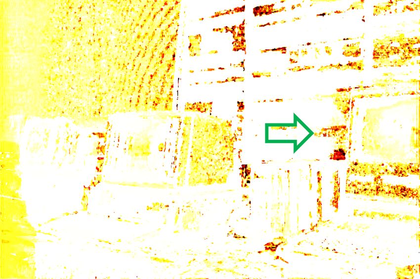
ISPRS Annals of the Photogrammetry, Remote Sensing and Spatial Information Sciences, Volume V-2-2021
                                             XXIV ISPRS Congress (2021 edition)

 Layer    Description                                     Output Tensor                                                   0.06
                                                           Dimensions

                                                                                                        probability [-]
 Input    Cost Volume Extract                             13×13×192                                                       0.04
                       Neighbourhood Fusion
 1        3D conv., 5×5×5, 32 filters                      9×9×188                                                        0.02
 2        3D conv., 5×5×5, 32 filters                      5×5×184
 3        3D conv., 5×5×5, 32 filters                      1×1×180
                          Depth Processing                                                                                  0
                                                                                                                             0    50     100 150
 4        3D conv., 1×1×8, 32 filters, zero pad.           1×1×180                                                               disparity [pixel]
 5        3D conv., 1×1×16, 32 filters, zero pad.          1×1×180
 6        3D conv., 1×1×32, 32 filters, zero pad.          1×1×180
 7-13     3D conv., 1×1×64, 32 filters, zero pad.          1×1×180         Figure 1. Illustration of the underlying assumptions of the
                       Uncertainty Estimation                              proposed geometry-aware model. On the left, the right image
 14       Global average pooling, linear act., no BN        1×1×32         of a stereo pair with a correct point match in a texture-less region
 15       3D conv., 1×1×1, 1 filter, linear act., no BN      1×1×1         and matching area in an occlued region are shown in blue and
                                                                           green, respectively. The considered search space is highlighted
Table 1. Summary of the modified CVA-Net architecture. Un-                 in red. On the right, the corresponding probability distributions
less otherwise specified, each layer is followed by batch norm-            over the considered disparity range are shown. The histograms
alisation (BN) and a ReLU non-linearity. (Adapted from (Mehl-              of the two cases, shown in blue and green, are approximated by
tretter and Heipke, 2021).)                                                Uniform distributions, shown in red and black.

ciated uncertainty, i.e. type and parameterisation of a particular         This model has already proven its suitability in the context
probability distribution, is typically not available. Neverthe-            of aleatoric uncertainty estimation for dense stereo match-
less, to be able to learn the task of uncertainty estimation, it           ing (Mehltretter and Heipke, 2021) and will therefore be used
is common to assume a specific uncertainty model, allowing                 as baseline in this work.
to implicitly learn uncertainty from the deviations between es-
timated and ground truth disparity. First, the Laplacian model,            3.2.2 Geometry-aware Model The previously described
considering the real error to be unimodally distributed, is re-            variant models the uncertainty contained in the data using a
viewed in Section 3.2.1, before two novel probabilistic models             Laplacian distribution. Assuming a unimodal error distribution
are proposed in Sections 3.2.2 and 3.2.3, taking challenging re-           for each pixel, the mode of such a distribution is designed to
gions of real-world scenarios and outlier measurements expli-              match with a unique and distinct global minimum in the corres-
citly into account. Besides different loss functions, also minor           ponding cost curve over the whole disparity range. However,
adjustments of the final network layer may be necessary to al-             this assumption is often not valid for all pixels in an image, due
low the prediction of varying numbers and types of values used             to the geometry or appearance of the depicted scene.
to parameterise these uncertainty models, explained in detail in
the respective paragraphs.                                                 In the context of dense stereo matching, a commonly challen-
                                                                           ging scenario is the presence of texture-less regions. A typical
3.2.1 Laplacian Model Under the assumption that the un-                    behaviour for pixel in such non- or weakly textured regions is
certainty contained in the data can be described with a spe-               the occurrence of a wide and flat minimum in the cost curve,
cific probability distribution, the parameters of this distribution        causing a wide and flat maximum in the corresponding prob-
can be inferred by maximising the likelihood (Kendall and Gal,             ability density function. This maximum can be described by a
2017). Similar to (Mehltretter and Heipke, 2021), we consider              range of (almost) uniform probability with a length correspond-
the disparity d estimated in advance and the predicted aleatoric           ing to the width of the non-textured region (cf. Fig. 1). Similar
uncertainty σ as the mean and standard deviation used to para-             to texture-less regions, also pixels in occluded regions, where
meterise a Laplacian distribution. In this context, the ground             some parts of a scene are not visible in one of the images of
truth disparity dˆ is used as observation. In this way, aleatoric          a stereo pair, may cause deviations from the assumption of a
uncertainty can be learned without the need for a reference of             unimodal probability density function. Because pixels in these
the uncertainty. By formulating the objective of this method as            regions do not have a correspondence, occluded pixels are often
the negative log likelihood of the Laplacian distribution as,              characterised by the absence of a distinct global minimum, but
                                                                           multiple local minima within an individual disparity interval in
                                    √                                      the corresponding cost curve. To better quantify the associated
                                     2
           − log p(dˆi | di ) ∝        |di − dˆi | + log(σi ),       (1)   uncertainty for these pixels, such a disparity interval should be
                                    σi
                                                                           kept as tight as possible, containing only pixels which belong
we enable the use of optimisation techniques commonly em-                  to the same object as the occluded one (cf. Fig. 1). In this
ployed to train neural networks. To make the training proced-              work, we assume that all disparities in such an interval have the
ure numerically more stable and to prevent the loss function               same probability to be correct. Note that this is a strong sim-
from being divided by zero, s = log(σ) is substituted in the               plification, since a uniform probability density function can not
loss function to predict the log standard deviation, as proposed           represent such local minima of a cost curve properly. To over-
by Kendall and Gal (2017). Finally, the loss function of the               come this limitation, a multimodal probability density function,
Laplacian model is defined as:                                             for example, described as Gaussian mixture model, would need
                                                                           to be employed to describe the characteristics contained in these
                            N   √                                          regions. However, this is beyond the scope of the present work
                          1 X     2
          LLaplacian =                 |di − dˆi | + si ,            (2)   and is subject of further investigations.
                          N   exp(si )
                              i=1
                                                                           As both, texture-less and occluded regions, are assumed to
where N is the number of training samples with known ground                be uniformly distributed in specific intervals in the probabil-
truth disparity.                                                           ity density function, a Laplacian distribution is not sufficient

         This contribution has been peer-reviewed. The double-blind peer-review was conducted on the basis of the full paper.
                     https://doi.org/10.5194/isprs-annals-V-2-2021-17-2021 | © Author(s) 2021. CC BY 4.0 License.                                    19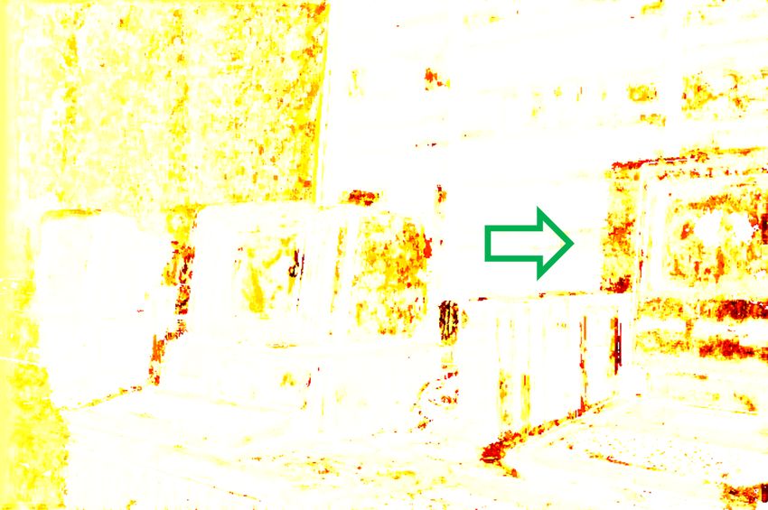
ISPRS Annals of the Photogrammetry, Remote Sensing and Spatial Information Sciences, Volume V-2-2021
                                             XXIV ISPRS Congress (2021 edition)

to model the uncertainty in these areas. Consequently, we use a       geometry-aware variant becomes:
Uniform distribution with a predictive interval in our geometry-
aware variant to model the uncertainty in these “hard” regions.                          N
                                                                                       1 X
Equal to the Laplacian variant described in Section 3.2.1, we          LGeometry* =        ĉi · LL + (1 − ĉi ) · LU + H(ci , ĉi ), (6)
                                                                                       N
consider the estimated disparity d as the mean of a Laplacian                             i=1

distribution and as the centre of an interval with Uniform dis-
                                                                            H(ci , ĉi ) = −ĉi · log(ci ) − (1 − ĉi ) · log(1 − ci ).   (7)
tribution, respectively. To achieve maximal probability, the
ground truth disparity dˆ needs to be included in the interval
[d − r, d + r], where r denotes the half interval length, without     3.2.3 Mixture Model While commonly challenging re-
motivating the network to predict unreasonable large intervals.       gions in the context of dense stereo matching are explicitly ad-
Thus, we maximise the likelihood with respect to the ground           dressed in our geometry-aware model, we treat aleatoric un-
truth disparity dˆ in these “hard” regions, by minimising the dif-    certainty from the perspective of measurement reliability in our
ference between the predictive half interval length r and the         mixture model presented in this section. According to Vogiatzis
absolute error of disparity estimation |d − d|ˆ.                      and Hernandez (2011) and Pizzoli et al. (2014), a depth sensor
                                     √                                produces two types of measurement: (1) a good measurement
Considering the relationship r = 3 σ between the half inter-          that is unimodally distributed around the correct depth or (2) an
val length r and the standard deviation σ of a Uniform distri-        outlier measurement that is drawn from a Uniform distribution
bution, we use the Huber loss (Huber, 1981), which combines           defined on a certain interval. Similar to the geometry-aware
the advantages of L1-loss (steady gradients for large values x)       model (see Sec. 3.2.2), we assume a Laplacian distribution for
and L2-loss (less oscillation during updates when x is small),        good measurements and a Uniform distribution with a predict-
to state the optimisation objective for the “hard” regions:           ive interval for outlier measurements. Thus, from the perspect-
                     (                                                ive of measurement reliability, aleatoric uncertainty can be de-
                         0.5x2            if |x| ≤ γ                  scribed as a mixture of a Laplacian and a Uniform distribution
              LU =                                             (3)    assigned a probability α and 1 − α, respectively.
                         γ|x| − 0.5γ 2    otherwise,
                                                                      Using the same optimisation objectives for both types of dis-
                          √
in which x = |di − dˆi | − 3 σi . In this work, we set γ to 1, as     tributions as in Section 3.2.2, the loss function of our mixture
commonly done in the literature (Mangasarian and Musicant,            model is defined as:
2000; Girshick, 2015).                                                                         N
                                                                                             1 X
                                                                                LMixture =       αi · LL + (1 − αi ) · LU ,               (8)
The cost curves of pixels located in none of the previously men-                             N
                                                                                                 i=1
tioned regions are usually characterised by a distinct global
minimum. This allows to reliably determine the correct pixel          where the inlier probability α is predicted by the network, to-
correspondence in most cases and thus leads to a lower un-            gether with the log standard deviations of the Laplacian dis-
certainty. Consequently, equal to the first variant, we use the       tribution sL and the Uniform distribution sU . The number of
Laplacian distribution to describe the uncertainty for pixels loc-    output nodes in the network architecture is therefore increased
ated in these “good” regions:                                         to three in this variant. To impose positive values and to ensure
                            √                                         that the inlier and outlier probabilities sum up to one, a softmax
                             2                                        transformation is applied to the α-node.
                 LL =             |di − dˆi | + si .           (4)
                         exp(si )
                                                                      In summary, this variant can be viewed as an extension of our
For the purpose of consistency, we also substitute s = log(σ)         geometry-aware model. In case that the inlier probability α is
for the objective of “hard” regions, so that our network is           predicted as 1 and 0 for “good” and “hard” regions respectively,
trained to predict the log standard deviation for both types of       both variants are equal (cf. Eq. 5 and Eq. 8). However, due to
regions and probability distributions. We therefore define the        the differences between the binary region parameter c in the
loss function of the geometry-aware variant as:                       geometry-aware model and the inlier probability α in the mix-
                                                                      ture model, the meaning of both variants is rather different.
                          N
                        1 X
          LGeometry =       ĉi · LL + (1 − ĉi ) · LU ,       (5)
                        N                                                              4. EXPERIMENTAL SETUP
                           i=1

                                                                      In order to investigate the influence of the different uncertainty
where ĉ denotes a binary parameter that is computed accord-
                                                                      models (cf. Sec. 3.2), we train and evaluate these three models
ing to (Scharstein and Szeliski, 2002) and discussed in detail in
                                                                      on three different datasets (discussed in detail in Section 4.1) as
Section 4.2. A pixel i gets assigned ĉi = 1 if it is located in a
                                                                      well as on cost volumes computed by two popular stereo match-
“good” region and 0 otherwise.
                                                                      ing methods: Census-based block matching (with a support re-
As the model described by Equation 5 does not learn to expli-         gion size of 5×5) (Zabih and Woodfill, 1994) and MC-CNN
citly predict the type of region a pixel is assigned to, the ground   fast (Zbontar et al., 2016). For the evaluation, we use two met-
truth region mask ĉ would be required in the test phase to allow     rics that are described in Section 4.4. To allow a fair compar-
a proper interpretation of the predicted uncertainty. However,        ison, all examined methods have been trained on the same data
because the determination of occluded regions requires ground         using the same network architecture, following the procedure
truth disparities, the model in its current form is not applicable    described in Section 4.3.
to real-world applications. To overcome this limitation, we ex-       4.1   Datasets
tend the loss function with a binary cross-entropy term H(c, ĉ),
allowing the model to also learn the prediction of the region         In this work, three datasets, namely KITTI 2012 (Geiger et al.,
mask c. Thus, the loss function of the real-world applicable          2012), KITTI 2015 (Menze and Geiger, 2015) and Middlebury

         This contribution has been peer-reviewed. The double-blind peer-review was conducted on the basis of the full paper.
                     https://doi.org/10.5194/isprs-annals-V-2-2021-17-2021 | © Author(s) 2021. CC BY 4.0 License.                         20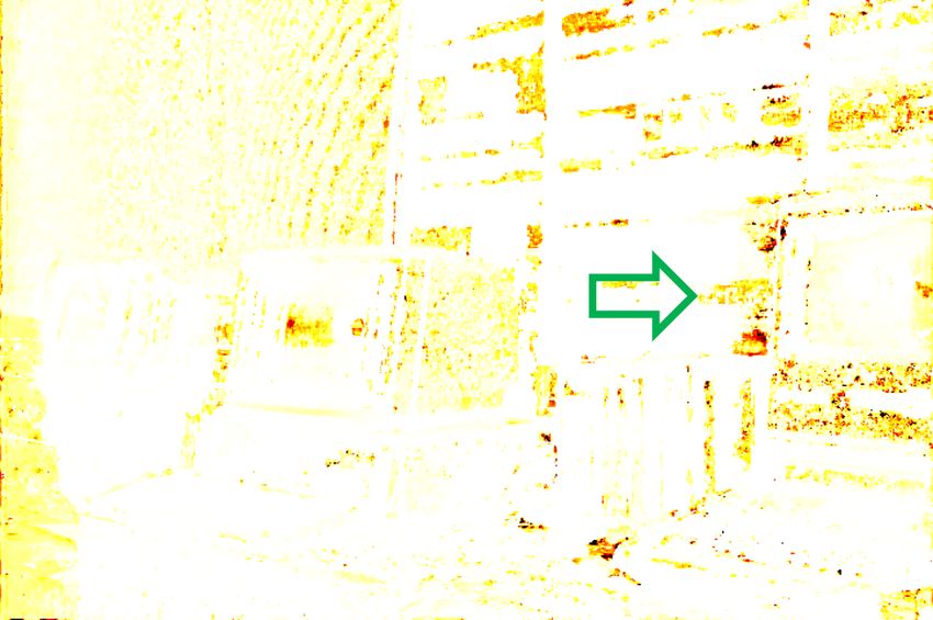
ISPRS Annals of the Photogrammetry, Remote Sensing and Spatial Information Sciences, Volume V-2-2021
                                               XXIV ISPRS Congress (2021 edition)

v3 (Scharstein et al., 2014) are used for the experiments. The                proposed by Hu and Mordohai (2012) to evaluate different con-
KITTI datasets consist of challenging and varied road scenes                  fidence estimation methods. In this context, a Receiver Oper-
captured from a moving vehicle. Ground truth disparity maps                   ating Characteristic (ROC) curve, for which the AUC is com-
for training and evaluation are obtained from LIDAR data with                 puted, represents the error rate as a function of the percentage
disparities for about 30% of the pixels. In contrast to the KITTI             of pixels sampled from a disparity map in order of increasing
datasets, the Middlebury dataset contains 15 image pairs show-                uncertainty. The error rate is defined as the percentage of pixels
ing various indoor scenes captured with a static stereo set-up                with a disparity error smaller than 3 pixels or 5% of the ground
and provides dense and highly accurate ground truth disparity                 truth disparities (Menze and Geiger, 2015). The optimal AUC
maps based on structured light.                                               depends only on the overall error  of a disparity map:
                                                                                                          Z    1
4.2     Binary Region Masks                                                                                         p − (1 − )
                                                                                             AU Copt =                          dp
                                                                                                              1−        p                   (9)
For the training procedure of the geometry-aware uncertainty                                           =  + (1 − )ln(1 − ),
model discussed in Section 3.2.2, binary region masks are
needed, which indicate with 1 and 0, respectively, whether a                  where p is the percentage of pixels sampled from a disparity
pixel is located in a “good” or a “hard” region. Since the ground             map. The closer the AUC of an uncertainty map gets to the
truth disparity maps of the KITTI datasets are not dense, masks               optimal value, the higher the accuracy.
for depth discontinuities cannot be computed accurately. In this
work, we therefore consider texture-less regions and occluded                 The downside of the AUC metric is that it only considers the
areas as “hard” regions with the following definitions:                       ratio of correct disparity estimates and the relative order of the
                                                                              estimated uncertainty values, while it simply neglects the ac-
    • Texture-less regions: regions in which the squared hori-                tual magnitude of the estimated uncertainty and thus also the
      zontal intensity gradient averaged over a 3×3 window is                 relation between this estimates and the real disparity error. To
      smaller than 4.0 (Scharstein and Szeliski, 2002).                       overcome this limitation, we therefore use the correlation coef-
                                                                              ficient between the absolute disparity error and the estimated
    • Occluded areas: occlusion can be determined from ground                 uncertainty as an additional metric to evaluate the uncertainty
      truth disparity maps directly, but the corresponding masks              models discussed. The higher the correlation, the better the un-
      are also already provided as part of all three datasets.                certainty can be quantified.

Pixels located in none of these two types of “hard” regions are               4.5   Evaluation Procedure
in turn labelled as “good”.
                                                                              To ensure a clear separation of training and test data, we evalu-
4.3     Training Procedure                                                    ate the three uncertainty models, which are trained on the KITTI
                                                                              2012 dataset, on the KITTI 2015 and Middlebury v3 datasets.
Following the description in (Mehltretter and Heipke, 2021), we               According to (Mehltretter and Heipke, 2021), the depth of the
train the three uncertainty models on the first 20 training image             input cost volume for the network is set to 192 pixels and the
pairs of the KITTI 2012 dataset (Geiger et al., 2012) and use                 image resolution is halved during testing, as long as the max-
three additional image pairs for validation. As input for the net-            imum disparity exceeds 192. Thus, the cost volumes of the
work, tensors of size 13×13×192 are extracted from normal-                    Middlebury dataset correspond to images with one quarter of
ised cost volumes corresponding to the left image of each pair.               the original resolution, whereas on the KITTI 2015 dataset,
The values contained in these cost volumes are normalised to                  cost volumes correspond to images in the original resolution.
[0, 1] using min-max normalisation. Every extract is centred on               Moreover, since the geometry-aware model assumes different
a pixel with available ground truth disparity. 128 of such ex-                uncertainty models for “good” and “hard” regions within a
tracts are bundled to one mini-batch and fed to the network per               scene, respectively, we distinguish between these two types of
forward pass during training.                                                 regions in our complete evaluation to allow a fair comparison.

We initialise the convolutional layers with normal distributions
                                                                                                       5. RESULTS
N (0, 0.0025) and use the Adam optimiser (Kingma and Ba,
2015) with its parameters set to their default values. The
learning rate is set to 10−4 . To enforce generalisation, dro-                In this section, the results of two different sets of experiments
pout (Srivastava et al., 2014) is applied to the global average               are analysed and discussed. First, we investigate the applicab-
pooling layer (layer 14, cf. Tab. 1) with a rate of 0.5. The train-           ility and compare the two variants of the proposed geometry-
ing procedure is stopped, if the validation loss did not decrease             aware model introduced in Section 3.2.2. Subsequently, the
in three consecutive epochs and the weights showing the lowest                ideal geometry-aware variant, i.e. the geometry-aware model
validation loss are used for testing. Thus, we trained the mod-               with “perfect” region assignments, and the proposed mixture
ified CVA-Net for 20, 17 and 19 epochs for the Laplacian, the                 variant are compared against the state-of-the-art Laplacian vari-
geometry-aware 1 and the mixture model, respectively.                         ant in Section 5.2, in order to verify the validity of the proposed
                                                                              uncertainty models.
4.4     Metrics
                                                                              5.1   Analysis of the Geometry-aware Approach
The first metric we use to evaluate the methodology presented
                                                                              To verify the applicability of the geometry-aware approach in
in this paper, is the Area Under the Curve (AUC), originally
                                                                              real-world applications, the variant with region mask prediction
1   If not otherwise specified, in this paper the term geometry-aware model   is first compared with the ideal variant, which has “perfect” re-
    refers to the model predicting uncertainty only.                          gion assignments for all pixels, using the correlation coefficient.

            This contribution has been peer-reviewed. The double-blind peer-review was conducted on the basis of the full paper.
                        https://doi.org/10.5194/isprs-annals-V-2-2021-17-2021 | © Author(s) 2021. CC BY 4.0 License.                          21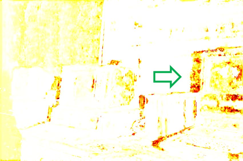
ISPRS Annals of the Photogrammetry, Remote Sensing and Spatial Information Sciences, Volume V-2-2021
                                             XXIV ISPRS Congress (2021 edition)

            Correlation    Geometry         Geometry*                   [%]                         KITTI 2015              Middlebury v3
            coefficient  good hard         good hard                                          ACC      TPR     TNR        ACC   TPR     TNR
               KITTI 2015 Menze and Geiger (2015)                       Census-BM            80.69    89.94    59.26      74.99    89.92   62.85
            Census-BM     0.84 0.80        0.83 0.80                    MC-CNN               84.07    91.10    67.78      78.34    69.09   85.85
            MC-CNN        0.73 0.73        0.69 0.72
               Middlebury v3 Scharstein et al. (2014)                 Table 3. Accuracy (ACC), true positive rate (TPR) and true
            Census-BM     0.82 0.81        0.79 0.78                  negative rate (TNR) of the region mask predictions of the
            MC-CNN        0.71 0.78        0.70 0.75                  real-world applicable geometry-aware model. The TPR and
                                                                      TNR measure the proportions of pixels that are correctly assigned
Table 2. Comparison of the two variants of the proposed               to the “good” and “hard” regions, respectively. For details on the
geometry-aware model based on the correlation coefficient.            evaluation procedure, please refer to Table 2.
The model marked with an asterisk jointly predicts an uncertainty
map and a region mask, whereas the second variant predicts un-                               Optimal
certainty values only. The results are based on the first 100 im-                  30
                                                                                             Laplacian
ages of the KITTI 2015 dataset and all images of the Middlebury                              Geometry
v3 dataset, except for the configuration MC-CNN + Middlebury                                 Mixture

                                                                       error [%]
                                                                                   20
v3. Due to a noticeable domain gap for this configuration, we
fine-tune the network on the first 4 images and test on the last 10
images of the Middlebury v3 dataset.                                               10

As shown in Table 2, the variant with region mask prediction                        0
(marked with an asterisk) shows a slight deterioration of the                           0    20          40          60           80       100
uncertainty quantification, but the results are still comparable                                         density [%]
to those of the ideal variant. These differences are probably due                           (a) ROC curves for “good” regions
to the increased complexity of the learning task caused by the                     60
additional consideration of the cross-entropy term in the loss                               Optimal
function.                                                                                    Laplacian
                                                                                   40        Geometry
For a further investigation, the region masks predicted by the                               Mixture
                                                                       error [%]

variant marked with an asterisk are evaluated using the over-
all accuracy (ACC), the true positive rate (TPR) and the true                      20
negative rate (TNR), with TPR and TNR describing the pro-
portions of pixels that are correctly assigned to the “good” and
“hard” regions, respectively. As shown in Table 3, the propor-                      0
tion of correctly assigned pixels is clearly higher in “good” re-                       0    20          40          60           80       100
gions than in “hard” ones in almost all configurations evaluated.                                        density [%]
Due to a noticeable domain gap for the configuration MC-CNN                                 (b) ROC curves for “hard” regions
+ Middlebury v3, the network is fine-tuned (see Tab. 2 for de-
tails) resulting in a TNR higher than the TPR for this configur-      Figure 2. ROC curves for the first 100 images of the KITTI
ation. This effect is probably caused by the higher percentage        2015 dataset and Census-based block matching. The closer
of “hard” samples in the Middlebury v3 dataset compared to            the curve of an uncertainty model reaches the optimal curve, the
the KITTI 2012 dataset, which is used to train all other vari-        higher the accuracy. The areas under these curves correspond to
ants and in which the majority of pixels are assigned to “good”       the AUC values in Table 4a.
regions. Consequently, the region mask prediction seems to
be very sensitive to the imbalanced occurrence of classes in
the training data. Addressing this class imbalance problem, a         variant are first analysed along with the state-of-the-art Lapla-
weighted cross-entropy term could be utilised to prevent the          cian variant with respect to the AUC metric (see Sec. 4.4). As
network from learning to preferably predict the more frequent         shown in Table 4a, the AUC values of “hard” regions are always
class. Moreover, because the computation of the texture-less re-      significantly larger than the values of “good” regions, indicating
gion masks is solely based on the stereo images which are also        the higher error rate of “hard” regions, which can also be seen
available during testing, these masks can be computed before-         in the ROC curves (cf. Fig. 2). This observation confirms that
hand and do not need to be predicted by the network. Con-             these “hard” regions are especially challenging for dense stereo
sequently, the region classification would be reduced to the          matching procedures, which is the fundamental motivation for
identification of occluded pixels, which simplifies the learn-        our geometry-aware uncertainty model that explicitly accounts
ing task. Together with the prior knowledge with respect to           for these regions. On the other hand, the differences among
the texture-less regions, the overall accuracy of the mask pre-       the three uncertainty models with respect to the AUC values
diction is expected to be further improved. To conclude, the          shown in Table 4a are not distinct. On all evaluated combina-
geometry-aware approach has shown its potential and applicab-         tions of disparity methods and datasets the results of the three
ility to real-world applications. However, further investigations     models are relatively similar. While the same can be observed
are required that will be carried out in future work.                 in Figure 2, it can also be seen that our geometry-aware model
                                                                      performs slightly better in detecting erroneous depth estimates
5.2   Uncertainty Model Evaluation                                    in the region of medium density and a bit worse in the region of
                                                                      low density compared to the Laplacian baseline.
To verify the validity of the approaches proposed earlier in this
work (see Sec. 3.2), the ideal geometry-aware and the mixture         As already mentioned in Section 4.4, the AUC metric neglects

         This contribution has been peer-reviewed. The double-blind peer-review was conducted on the basis of the full paper.
                     https://doi.org/10.5194/isprs-annals-V-2-2021-17-2021 | © Author(s) 2021. CC BY 4.0 License.                                22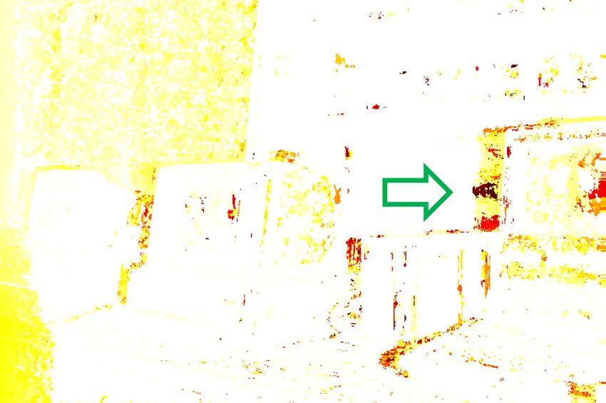
ISPRS Annals of the Photogrammetry, Remote Sensing and Spatial Information Sciences, Volume V-2-2021
                                                        XXIV ISPRS Congress (2021 edition)

       avg. AUC                 Opt.        Laplacian          Geometry                   Mixture             Correlation   Laplacian      Geometry           Mixture
       = 10−2 ×            good     hard  good    hard       good     hard             good    hard           coefficient  good hard     good hard         good hard
                                 KITTI 2015 Menze and Geiger (2015)                                                     KITTI 2015 Menze and Geiger (2015)
       Census-BM           5.69 22.13     7.94 28.05         7.92 27.83                 8.10   27.96          Census-BM    0.74 0.72     0.84 0.80          0.78 0.77
       MC-CNN              1.06     7.19  2.19 10.35         2.40 11.04                 2.27   10.27          MC-CNN       0.70 0.70     0.73 0.73          0.71 0.70
                                 Middlebury v3 Scharstein et al. (2014)                                                Middlebury v3 Scharstein et al. (2014)
       Census-BM           1.66 14.26     3.38 18.70         3.68 18.89                 3.70   18.87          Census-BM    0.73 0.71     0.82 0.81          0.79 0.79
       MC-CNN              0.51     8.94  1.51 12.03         1.44 11.59                 1.36   12.09          MC-CNN       0.68 0.71     0.71 0.78          0.70 0.74

(a) AUC comparison. The values represent the AUC×10−2 , whereas the                                          (b) Correlation coefficient comparison, measuring the
smaller the values, the better, while Opt. is the best achievable value (cf.                                 correlation between the absolute disparity error and the
Sec. 4.4).                                                                                                   estimated uncertainty. The bigger the values, the better.

Table 4. Comparison of the three uncertainty models. For details on the evaluation procedure, please refer to Table 2. While the
three uncertainty models have only minor differences based on the AUC metric, the proposed geometry-aware model exceeds other
models by a wide margin considering the correlation coefficient metric.
                        0.01% 0.1%      1%      10%                                    0.01% 0.1%      1%     10%                                   0.01% 0.1%      1%      10%

             600                                                         150                                                             400
                                                                                                                                         300
SD [pixel]

                                                            SD [pixel]

                                                                                                                            SD [pixel]
             400                                                         100
                                                                                                                                         200
             200                                                          50
                                                                                                                                         100
              0                                                           0                                                               0
               0        50      100       150       200                    0        50      100       150       200                        0        50      100       150       200
                   Absolute Disparity Error [pixel]                            Absolute Disparity Error [pixel]                                Absolute Disparity Error [pixel]

                           0.01% 0.1%      1%    10%                                    0.01% 0.1%      1%     10%                                     0.01% 0.1%      1%    10%

             600                                                         150                                                             400
                                                                                                                                         300
                                                            SD [pixel]
SD [pixel]

                                                                                                                            SD [pixel]
             400                                                         100
                                                                                                                                         200
             200                                                         50
                                                                                                                                         100
              0                                                           0                                                               0
               0        50      100       150       200                    0        50      100       150       200                        0        50      100       150       200
                   Absolute Disparity Error [pixel]                            Absolute Disparity Error [pixel]                                Absolute Disparity Error [pixel]
                        (a) Laplacian model                                         (b) Geometry model                                               (c) Mixture model

Figure 3. Absolute error uncertainty relation. The results are based on the first 100 images of the KITTI 2015 dataset using cost
volumes computed with Census-based block matching. From top to bottom, the “good” and the “hard” regions are shown. The
logarithmic colour scale encodes the percentage of pixels showing the respective error and estimated standard deviation (SD).

the relation between the error magnitude and the predicted un-                                    ing this case is shown in Figure 4: In the “hard” regions, the
certainty by only considering the ability to separate correct from                                Laplacian model underestimates the uncertainty clearly for the
incorrect disparity assignments, which limits its expressiveness.                                 non-textured areas on the wall especially visible in the Census-
Thus, we additionally investigate the relation between the abso-                                  based uncertainty maps. The same behaviour can be observed
lute disparity error of a pixel and the corresponding predicted                                   for the occluded area behind the right computer (highlighted by
uncertainty using the correlation coefficient. Analysing the cor-                                 a green arrow) in the uncertainty maps for both disparity meth-
relation coefficients presented in Table 4b, it can be seen that                                  ods. On the other hand, the Laplacian model also tends to as-
the two uncertainty models proposed in this work outperform                                       sign large uncertainties to pixels with a disparity error between
the state-of-the-art Laplacian model in all configurations evalu-                                 0 and 50 pixels, which is not the case for the two models pro-
ated. Especially the geometry-aware model exceeds the Lapla-                                      posed in this work (see Fig. 3). An example of this behaviour
cian one by a wide margin, which can also be seen in Figure 3:                                    can be seen in the Census-based uncertainty maps correspond-
While the heatmaps of the Laplacian and the mixture model are                                     ing to hard regions shown in Figure 5: Compared to the other
more dispersed for both “good” and “hard” regions, the results                                    models and the error map, the Laplacian model generates rel-
of the geometry-aware model shows significantly stronger cor-                                     atively noisy uncertainty estimates in the areas of the door and
relations between the absolute disparity error and the predicted                                  back of the car containing some extremely high values.
uncertainty. This supports our assumption regarding occluded
and texture-less regions and demonstrates the benefit of addi-                                    According to the “good” regions in Figure 4, it can be seen that
tionally introducing a Uniform distribution to the loss term.                                     the uncertainties of pixels located at object boundaries (high-
                                                                                                  lighted by a red arrow) are less accurate for all uncertainty mod-
Figure 3 further shows that the Laplacian model tends to as-                                      els and for both disparity methods. This problem is caused by
sign small uncertainties to pixels with a large disparity error,                                  two potential reasons: First, the KITTI dataset, which was used
especially visible for the “hard” regions. An example illustrat-                                  for training, provides a sparse ground truth for the disparities

                     This contribution has been peer-reviewed. The double-blind peer-review was conducted on the basis of the full paper.
                                 https://doi.org/10.5194/isprs-annals-V-2-2021-17-2021 | © Author(s) 2021. CC BY 4.0 License.                                                         23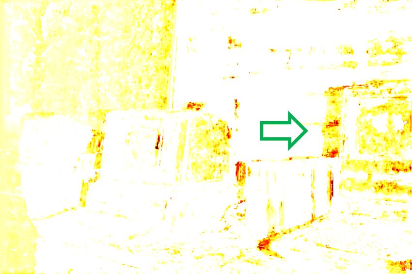
ISPRS Annals of the Photogrammetry, Remote Sensing and Spatial Information Sciences, Volume V-2-2021
XXIV ISPRS Congress (2021 edition)
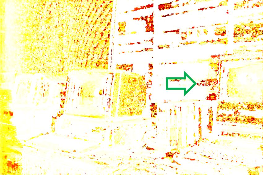
(a) Reference images (b) Error maps (c) Laplacian model (d) Geometry model (e) Mixture model
Figure 4. Qualitative uncertainty evaluation on the Middlebury v3 dataset. From top to bottom, the “good” and the “hard” regions
based on Census-BM and MC-CNN disparity methods are shown. The error and the uncertainty maps encode a high value in black
and a small one in white. Note that also pixels without ground truth disparities are displayed in white. To allow a clear illustration
of the spatial distribution of uncertainty, all uncertainty maps are normalised. In general, the proposed geometry model and mixture
model show superior results in the “hard” regions, e.g. in the areas highlighted by green arrows, while uncertainties close to depth
discontinuities (highlighted by red arrows) are less accurate for all three uncertainty models.
and our network is trained in a supervised manner, only us- perior compared to the unimodal baseline, which is especially
ing patches centred on pixels with known ground truth. Con- visible for occluded and texture-less areas of an image. How-
sequently, edges in the disparity space caused by depth discon- ever, the prediction of regions masks shows potential to be fur-
tinuities are rarely seen by the network during training. Second, ther improved, for example, by addressing the problem of im-
the assumed Laplacian or Laplace-Uniform mixture distribu- balanced training data and the direct derivation of texture-less
tion is not suitable to describe the uncertainty related to depth regions from the reference image. Moreover, the results have
discontinuities properly. In this case, it may be beneficial to util- also shown that the two presented models as well as the baseline
ise a multimodal distribution for the estimation of uncertainty are less accurate for pixels close to depth discontinuities. To
at depth discontinuities. However, further investigations on that overcome this limitation, we plan to further investigate the pos-
topic are necessary and will be carried out in future work. sibilities of employing multimodal distributions, for example,
in form of a Gaussian mixture model, to improve the estimation
6. CONCLUSION of aleatoric uncertainty in these areas.
In the present work, we propose two novel mixed probabil- ACKNOWLEDGEMENTS
ity models for the task of aleatoric uncertainty estimation in
the context of dense stereo matching. For this purpose, we This work was supported by the German Research Founda-
explicitly consider commonly challenging regions and outlier tion (DFG) as a part of the Research Training Group i.c.sens
measurements employing mixtures of a Laplacian and a Uni- [GRK2159] and the MOBILISE initiative of the Leibniz Uni-
form distribution. We argue that real-world scenarios typically versity Hannover and TU Braunschweig.
violate the assumption of a unimodal distribution, commonly
assumed by probabilistic uncertainty models in the literature.
Thus, mixed probability models are better suited to describe the References
uncertainty inherent in such scenarios. In our experiments, we
use the architecture of CVA-Net, which utilises cost volume as Batsos, K., Cai, C., Mordohai, P., 2018. CBMV: A Coalesced
input data, to investigate the effects of the proposed uncertainty Bidirectional Matching Volume for Disparity Estimation. Pro-
models. We evaluate the performance of these models on two ceedings of the IEEE Conference on Computer Vision and Pat-
different datasets using cost volumes originating from two dif- tern Recognition, 2060–2069.
ferent dense stereo matching methods.
Fu, Z., Ardabilian, M., Stern, G., 2019. Stereo Matching Con-
The results of the two proposed models demonstrate to be su- fidence Learning Based on Multi-modal Convolution Neural
This contribution has been peer-reviewed. The double-blind peer-review was conducted on the basis of the full paper.
https://doi.org/10.5194/isprs-annals-V-2-2021-17-2021 | © Author(s) 2021. CC BY 4.0 License. 24
ISPRS Annals of the Photogrammetry, Remote Sensing and Spatial Information Sciences, Volume V-2-2021
                                            XXIV ISPRS Congress (2021 edition)

   (a) Reference images          (b) Error maps           (c) Laplacian model      (d) Geometry model          (e) Mixture model

Figure 5. Qualitative uncertainty evaluation on the KITTI 2015 dataset. From top to bottom, the “good” and the “hard” regions
based on Census-BM and MC-CNN disparity methods are shown. For details on the colour coding, please refer to Fig. 4. The
uncertainty maps based on Census-BM generated by the two proposed models are smoother at the texture-less rear of the car, while the
Laplacian model generates noisy uncertainties in this area.

Networks. Representations, Analysis and Recognition of Shape         Mehltretter, M., Heipke, C., 2021. Aleatoric Uncertainty Estim-
and Motion from Imaging Data, Springer, Cham, 69–81.                 ation for Dense Stereo Matching via CNN-based Cost Volume
                                                                     Analysis. ISPRS Journal of Photogrammetry and Remote Sens-
Geiger, A., Lenz, P., Urtasun, R., 2012. Are we ready for            ing, 63–75.
Autonomous Driving? The KITTI Vision Benchmark Suite.
Proceedings of the IEEE Conference on Computer Vision and            Menze, M., Geiger, A., 2015. Object Scene Flow for Autonom-
Pattern Recognition, 3354–3361.                                      ous Vehicles. Proceedings of the IEEE Conference on Com-
                                                                     puter Vision and Pattern Recognition, 3061–3070.
Girshick, R., 2015. Fast R-CNN. IEEE International Confer-
ence on Computer Vision, 1440–1448.                                  Pizzoli, M., Forster, C., Scaramuzza, D., 2014. REMODE:
                                                                     Probabilistic, Monocular Dense Reconstruction in Real Time.
Hu, X., Mordohai, P., 2012. A Quantitative Evaluation of Con-        Proceedings of the IEEE International Conference on Robotics
fidence Measures for Stereo Vision. IEEE transactions on pat-        and Automation, 2609–2616.
tern analysis and machine intelligence, 34(11), 2121–2133.
                                                                     Poggi, M., Aleotti, F., Tosi, F., Mattoccia, S., 2020. On the
Huber, P. J., 1981. Robust Statistics. Wiley, New York.
                                                                     Uncertainty of Self-Supervised Monocular Depth Estimation.
Kendall, A., Gal, Y., 2017. What Uncertainties Do We Need            Proceedings of the IEEE Conference on Computer Vision and
in Bayesian Deep Learning for Computer Vision? Advances in           Pattern Recognition, 3227–3237.
Neural Information Processing Systems, 5574–5584.
                                                                     Poggi, M., Mattoccia, S., 2016. Learning from scratch a confid-
Kingma, D. P., Ba, J., 2015. Adam: A Method for Stochastic           ence measure. Proceedings of the British Machine Vision Con-
Optimization. Proceedings of the International Conference on         ference, BMVA Press, 46.1–46.13.
Learning Representations.
                                                                     Scharstein, D., Hirschmueller, H., Kitajima, Y., Krathwohl, G.,
Lin, M., Chen, Q., Yan, S., 2014. Network In Network. Pro-           Nešić, N., Wang, X., Westling, P., 2014. High-resolution Stereo
ceedings of the International Conference on Learning Repres-         Datasets with Subpixel-accurate Ground Truth. German Con-
entations.                                                           ference on Pattern Recognition, Springer, 31–42.

Mangasarian, O., Musicant, D., 2000. Robust Linear and Sup-          Scharstein, D., Szeliski, R., 2002. A Taxonomy and Evaluation
port Vector Regression. IEEE Transactions on Pattern Analysis        of Dense Two-Frame Stereo Correspondence Algorithms. In-
and Machine Intelligence, 22, 950-955.                               ternational Journal of Computer Vision, 47(1), 7–42.

Mehltretter, M., Heipke, C., 2019. CNN-based Cost Volume             Srivastava, N., Hinton, G., Krizhevsky, A., Sutskever, I.,
Analysis as Confidence Measure for Dense Matching. Proceed-          Salakhutdinov, R., 2014. Dropout: A Simple Way to Prevent
ings of the IEEE International Conference on Computer Vision         Neural Networks from Overfitting. Journal of Machine Learn-
Workshops, 2070–2079.                                                ing Research, 15(56), 1929–1958.

         This contribution has been peer-reviewed. The double-blind peer-review was conducted on the basis of the full paper.
                     https://doi.org/10.5194/isprs-annals-V-2-2021-17-2021 | © Author(s) 2021. CC BY 4.0 License.                  25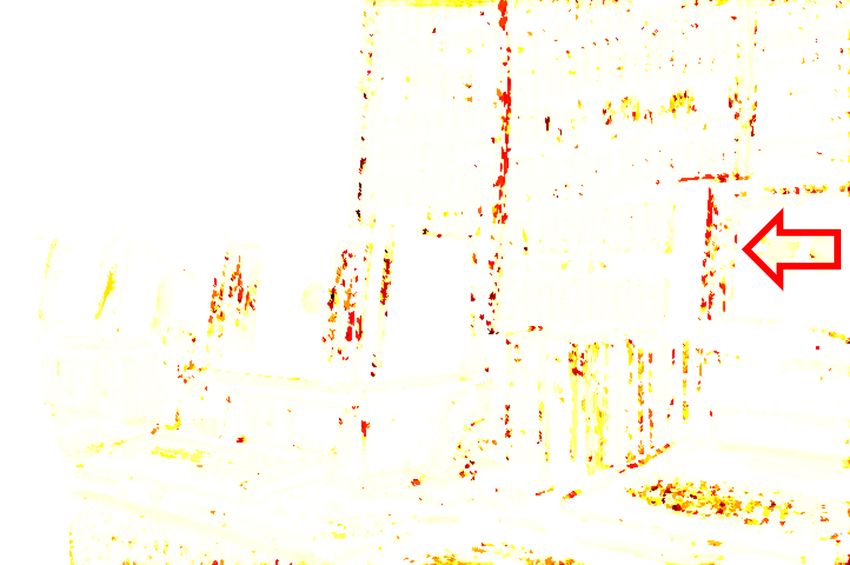
ISPRS Annals of the Photogrammetry, Remote Sensing and Spatial Information Sciences, Volume V-2-2021
                                            XXIV ISPRS Congress (2021 edition)

Sun, L., Chen, K., Song, M., Tao, D., Chen, G., Chen, C.,
2017. Robust, Efficient Depth Reconstruction With Hierarch-
ical Confidence-Based Matching. IEEE Transactions on Image
Processing, 26(7), 3331-3343.

Tosi, F., Poggi, M., Benincasa, A., Mattoccia, S., 2018. Beyond
Local Reasoning for Stereo Confidence Estimation with Deep
Learning. Proceedings of the European Conference on Com-
puter Vision, 319–334.

Vogiatzis, G., Hernandez, C., 2011. Video-based, Real-Time
Multi-View Stereo. Image and Vision Computing, 29(7).

Zabih, R., Woodfill, J., 1994. Non-Parametric Local Trans-
forms for Computing Visual Correspondence. Proceedings of
the European Conference on Computer Vision, Springer, 151–
158.

Zbontar, J., LeCun, Y. et al., 2016. Stereo matching by train-
ing a convolutional neural network to compare image patches.
Journal of Machine Learning Research, 17(1), 2287–2318.

         This contribution has been peer-reviewed. The double-blind peer-review was conducted on the basis of the full paper.
                     https://doi.org/10.5194/isprs-annals-V-2-2021-17-2021 | © Author(s) 2021. CC BY 4.0 License.               26
You can also read