Neural Improvement Heuristics for Preference Ranking - arXiv
←
→
Page content transcription
If your browser does not render page correctly, please read the page content below
Neural Improvement Heuristics for
                                                                 Preference Ranking

                                                         Andoni I. Garmendia, Josu Ceberio, Alexander Mendiburu
                                                             University of the Basque Country UPV/EHU, Spain
                                                    {andoni.irazusta,josu.ceberio,alexander.mendiburu}@ehu.eus
arXiv:2206.00383v1 [cs.AI] 1 Jun 2022

                                                                                     Abstract

                                                 In recent years, Deep Learning based methods have been a revolution in the field
                                                 of combinatorial optimization. They learn to approximate solutions and constitute
                                                 an interesting choice when dealing with repetitive problems drawn from similar
                                                 distributions. Most effort has been devoted to investigating neural constructive
                                                 methods, while the works that propose neural models to iteratively improve a
                                                 candidate solution are less frequent. In this paper, we present a Neural Improvement
                                                 (NI) model for graph-based combinatorial problems that, given an instance and a
                                                 candidate solution, encodes the problem information by means of edge features.
                                                 Our model proposes a modification on the pairwise precedence of items to increase
                                                 the quality of the solution. We demonstrate the practicality of the model by applying
                                                 it as the building block of a Neural Hill Climber and other trajectory-based methods.
                                                 The algorithms are used to solve the Preference Ranking Problem and results show
                                                 that they outperform conventional alternatives in simulated and real-world data.
                                                 Conducted experiments also reveal that the proposed model can be a milestone in
                                                 the development of efficiently guided trajectory-based optimization algorithms.

                                        1   Introduction
                                        Combinatorial Optimization Problems (COPs) are present in a broad range of real-world applications,
                                        such as logistics, manufacturing or biology [1]. Due to the NP-hard nature of most of the COPs,
                                        finding the optimal solution to medium/large sized problems is intractable [2]. As a result, in the
                                        last few decades, heuristic methods have been established as an alternative to approximate hard
                                        optimization problems in a reasonable amount of time. Despite being widely used, a major drawback
                                        of such methods is the need to exhaustively evaluate a large amount of candidate solutions.
                                        In the last decade, the rapid development of Deep Learning (DL) has enabled the creation of neural
                                        network-based models that can substantially decrease the computational effort in optimization. Two
                                        main frameworks can be distinguished: constructive methods and improvement methods. The former
                                        class generates a unique solution incrementally by iteratively adding an item to a partial solution
                                        until it is completed. Conversely, improvement methods take a candidate solution and suggest a
                                        modification to improve it. In fact, the improvement process can be repeated iteratively, using the
                                        modified solution as the new input of the model. These methods can potentially reduce the extensive
                                        search only focusing on trajectories leading to optimal solutions.
                                        In this paper we focus on improvement methods and propose a Neural Improvement (NI) model for
                                        graph-based combinatorial problems. This model encodes a given solution by means of edge features
                                        and proposes a modification on the pairwise precedence of some items, with the aim of obtaining a
                                        better candidate. To illustrate its usage, we apply the model to solve the Preference Ranking Problem
                                        (PRP), an NP-hard problem that tries to find an optimum pairwise consensus in a set of items.
                                        In particular, this paper makes the following contributions:

                                        Preprint. Under review.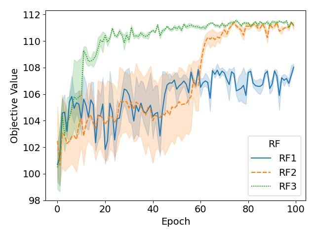
• Presents a Reinforcement Learning formulation for a Neural Improvement model parameter-
         ized by Graph Neural Networks and Attention Mechanisms.
       • Introduces a novel encoding-decoding process which considers as input both the stationary
         instance information and a candidate solution to be improved by means of the graph-edges.
       • Conducts an exhaustive analysis on the short-term (one improvement step) and long-term
         (multiple improvement steps) inference capabilities of the Neural Improvement model for
         the PRP. Moreover, we develop a Neural Hill Climbing based on the presented model and
         compare its performance to conventional procedures.
       • We demonstrate the applicability of the model by using it as the building block of two
         advanced Hill climbing methods: Tabu Search and Iterated Local Search.

2   Related Work
Neural Networks (NN) have been used since the decade of the 80s to solve COPs in the form of
Hopfield Networks [3]. However, as seen in recent surveys [4, 5], the growth in the computation
power and the development of advanced architectures in the last decade has enabled more efficient
applications that are getting closer to state-of-the-art algorithms. As mentioned previously, NN-based
optimization methods can be divided into two main groups according to their strategy.

Neural Constructive Methods Most of the DL-based works develop policies to learn a constructive
heuristic. These methods start from an empty solution and iteratively add an item to the solution
until a certain stopping criterion is met. One of the earliest works in the Neural Combinatorial
Optimization paradigm, Bello et al. [6] used a Pointer Network model [7] to parameterize a policy
that constructs a solution, item by item, for the Travelling Salesman Problem (TSP). Motivated by
the results in [6], and mainly focusing on the TSP, DL practitioners have successfully implemented
different architectures such as Graph Neural Networks [8, 9] or Transformers [10, 11].
As previously seen in the Operations Research literature, the solutions obtained by these proposals are
not competitive with state-of-the-art methods [12]. In fact, since the performance of these models is
still far from optimality (mostly in large size instances), they are usually enhanced with supplementary
algorithms that augment the solution diversity at the cost of increasing the computational time. A
common practice is to use active search [6], where rewards obtained from the evaluation instances
are used to fine-tune the parameters of a model. An alternative is to use sampling [6, 10] or beam
search [7] to further explore the neighborhood of the solution proposed by the model.

Neural Improvement Methods Improvement methods, also known as trajectory methods, are
initialized with a given solution, and iteratively propose a (set of) modification(s) to improve it until
the solution cannot be further improved. Neural Improvement (NI) methods utilize the learned policy
to navigate intelligently across the different neighborhoods.
To that end, the architectures used for constructive methods have been reused for implementing
improvement methods. Chen et al. [13] use LSTMs to parameterize two models: a model outputs
a score or probability to each region of the solution to be rewritten, while a second model selects
the rule that modifies that region. Lu et al. [14] use the Transformer model to select a local operator
among a pool of operators to solve the capacitated vehicle routing problem (VRP). Finally, Wu et al.
[15] use a similar architecture to train a policy that selects the node-pair to apply a local operator,
e.g., 2-opt.
Improvement methods not only incorporate the stationary instance data, but also need to consider the
present solution. In fact, the difficulty of encoding the solution information into a latent space to be
understandable to the model is a major challenge for most of the combinatorial problems.
In routing problems there are various ways of representing solutions. Each node (or city) can maintain
a set of features that indicate the relative position in the current solution, such as the location and
distance to the previously and subsequently visited nodes [14]. However, this technique does not
consider the whole solution as one, instead it only contemplates consecutive pairs of nodes in the
solution. A common alternative when using the transformer architecture is to incorporate Positional
Encodings (PE), which capture the sequence of the visited cities in a given solution [10]. Recently,
Ma et al. [16] propose a cyclic PE that captures the circularity and symmetry of the routing problem,
making it more suitable in representing solutions than the conventional PE.

                                                   2
Figure 1: Example of a PRP instance of size N = 5. a) A preference matrix of size N = 5 ordered as
the identity permutation ωe = (1 2 3 4 5). Entries of the matrix contributing to the objective function
are highlighted in grey, the sum of the entries in the upper diagonal gives the objective value, which
is 51. For this instance, the optimal solution is given by the permutation ωopt = (4 1 2 5 3) with an
objective value of 60. b) Equivalent complete graph with edge weights; only the edges of the first
node are shown for clarity. c) Identity permutation represented as the solution graph.

However, in some graph problems, the edges can provide useful information that it is not contained in
the nodes, namely, the relative information among nodes. Moreover, in some problems the essential
information is codified in edges, and thus, prior methods that focus on node embeddings [14, 16]
are not capable of properly encoding the relative information. In the following section, we will
present the optimization problem that illustrates the need to develop neural models that consider edge
features.

3   Preference Ranking Problem

Ranking items based on preferences or opinions is, in general, a straightforward task if the number of
alternatives to rank is relatively small. Nevertheless, as the number of alternatives/items increases, it
becomes harder to get full rankings that are consistent with the pairwise item-preferences. Think of
ranking 50 players in a tournament using their paired comparisons from the best performing player to
the worst. Obtaining the ranking that agrees with most of the pairwise comparisons is not trivial. This
task is known as the Preference Ranking Problem (PRP) [17]. Formally, given a preference matrix
B = [bij ]N ×N where entries of the matrix bij represent the preference of item i against item j, the
aim is to find the simultaneous permutation of rows and columns of B so that the sum of entries in
the upper-triangle of the matrix is maximized (see Eq. 1).

Note that row i describes the preference vector of
                                                                          N −1   N
item i over the rest of N − 1 items, while column                         X      X
i denotes the preference of the rest of the items               f (ω) =               bω(i)ω(j)      (1)
over item i. Thus, in order to maximize the up-                           i=1 j=i+1
per triangle of the matrix, preferred items must
precede in the ranking (see Fig.1 a).

Alternatively, the problem can be formulated as a complete bidirected graph where nodes represent the
set of items to be ranked and the weighted edges denote the preference between items. A pair of nodes
i and j has two connecting edges (i, j) and (j, i), with weights bij and bji that form the previously
mentioned preference matrix B. A solution (permutation) to the PRP can be also represented as an
acyclic tournament on the graph, where the node (item) ranked first has only outgoing edges, the
second in the ranking has 1 incoming edge and the rest are outgoing, and so on until the last ranked
node, which only has incoming edges (see Fig.1 b and c).

Applications Ranking from pairwise comparisons is a ubiquitous problem in modern Machine
Learning research. It has attracted the attention of the community due to its applicability in various
research areas, including but not being limited to: machine translation [18], economics [19], corrup-
tion perception [20] or any other task requiring a ranking of items, such as sport tournaments, web
search, resource allocation and cybersecurity [21, 22, 23].

                                                     3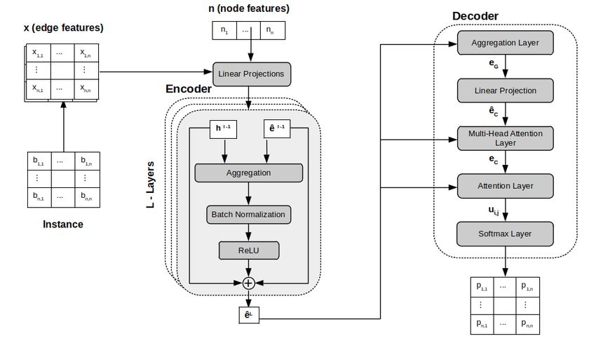
Figure 2: Architecture of the NI model.

4         Method
Reinforcement Learning: Markov Decision Process The idea of solving the PRP iteratively with
a NI model can be formulated as a Markov Decision Process (MDP), where a policy π is responsible
for selecting an action a at each step t based on a given state st of the problem. The main entities of
the MDP in this work can be described as:

      • State. A state st represents the information of the environment at step t. In this case, the state
        gathers data from two information sources: (1) stationary data, which the PRP instance to be
        solved, and (2) dynamic data, that is, a candidate solution ω to the problem at step t.
      • Action. At every step, the learnt policy selects an action at , which involves a pair of items that,
        according to the policy, are incorrectly ranked. Once selected, an operator is applied that alters
        the precedences of one, both or more items1 .
      • Reward. The transition between states st and st+1 is derived from an local operator applied in
        a pair of items given by at . The reward function represents the improvement of the solution
        quality across states. Different function designs can be used, as will be explained in Section 4.2.

4.1       NI Model

We will parameterize the policy π as a NN model with trainable parameters θ. Fig. 2 presents the
general architecture of the model, composed of two sub-models: an encoder and a decoder.

Encoder Given a graph instance of size N that represents a PRP, there are N × N edges or node
pairs, and each edge (i, j) represents the precedence of node i with respect to node j. Note that only
N × (N − 1) edges need to be considered since edge (i, i) does not provide any useful information.
As previously noted, the policy considers both instance information (stationary) and a candidate
solution at time step t (dynamic). For this purpose, we will use a bi-dimensional feature vector
xij ∈ R2 for each edge (i, j). The first dimension in xij denotes the element bij of the preference
matrix when node i precedes node j in the solution, and it is set to zero otherwise. Similarly, the
second dimension denotes the element bji of the preference matrix when node j precedes node i in
the solution, and it is set to zero otherwise.
Conversely, nodes do not reflect any problem-specific information. In fact, following a similar
strategy to that proposed by Kwon et al. [24], we select to use vectors of ones as node features
n ∈ RN . Even though all nodes are initiated with the same value, these features will help to spread
edge features across the graph in the encoding: node i will gather information from edges ik and ki
where k : {1, ..., N }.
      1
    The terms preference and precedence are interchangeably used throughout the paper as the preference
between two items is translated to have a precedent position in the solution ω.

                                                      4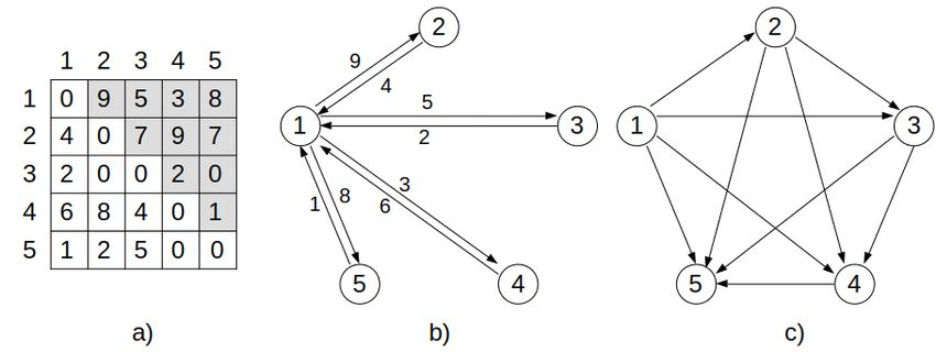
Node and edge features will be linearly projected to produce d-dimensional node hi and edge eij
embeddings
hi = ni ∗ Vh + Uh (2)
T
eij = xij ∗ Ve + Ue (3)
where Ve ∈ R2×d and Vh , Ue and Uh ∈ R1×d are learnable parameters.
The encoding process consists of L Graph Neural Network (GNN) layers (defined by the superscript
l) that perform a sequential message passing between nodes and their connecting edges (see left
part of Fig. 2). Eqs. 4 and 5 define the message passing in each layer, where W1l , W2l , W3l , W4l and
W5l ∈ Rd×d are learnable parameters, BN denotes the batch normalization layer, σ is the sigmoid
function and is the Hadamard product.
N
X
hl+1
i = hli + ReLU BN W1l hli + (σ(elij ) W2l hlj ) (4)
j=1
el+1 l l l l l l l
ij = eij + ReLU BN W3 eij + W4 hi + W5 hj (5)
The output of the encoder, which is fed to the decoder, consists of the edge embeddings of the last
1
PN PN L
layer eL
ij , plus the graph embedding eG = N 2 i=1 j=1 eij , which is an aggregation of the edge
embeddings.
Decoder Graph embeddings are projected to form the query (Q = Wg eG ) of a multi-head attention
mechanism (MHA) [25]. The MHA mechanism measures the compatibility of the query with each one
of the keys or edge embeddings (K = V = eij ). The output is a context vector ec = MHA(Q, K, V )
that is again refined in a second attention layer to produce the logits uij ;
(WQ ec )T ·(WK eL
ij )
C · tanh √ if i 6= j
uij = d (6)
−∞ otherwise
where the tanh function is used to maintain the logits within [−C, C] (C = 10). The logits are then
normalized using the Softmax function to produce a matrix p ∈ RN ×N which gives the probability of
modifying the precedence between items i and j. The model will be set to sample from the probability
matrix during training and to select the action with maximum probability during inference.
4.2 Learning
Loss Function The improvement policy will be learned using the REINFORCE algorithm [26].
Given a state st = (B, ωt ) which includes an instance and a candidate solution at step t, the model
gives a probability distribution pθ (at |st ) of all the possible pairwise preferences to be modified. After
performing an operation O(ωt |at ) = ωt+1 with the selected pair, a new solution ωt+1 is obtained.
The training is performed minimizing the loss function
L(θ|s) = Epθ (s,ωt ) [−Rt log pθ (s, ωt )] (7)
−1
TP
by gradient descent, where Rt = γ i (ri − ri−1 ) corresponds to the sum of cumulative rewards ri
i=0
with a decay factor γ in an episode of length T (see Appendix A for further details).
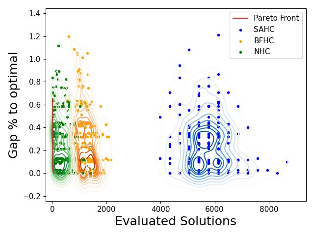
In order to obtain r, different Reward Functions (RF) can be found in the literature. Lu et al. [14]
use a reward function (RF1) that takes the objective value of the initial solution as the baseline and,
for each subsequent action, the reward at step t is defined as the difference between f (ωt ) and the
baseline. The drawback of this function is that rewards may get larger and larger and even bad moves
far from the baseline can be defined as positive rewards.
Alternatively, the most common approach in recent works [15, 16], is to define the reward (RF2) as
rt = max[f (ωt+1 ), f (ω ∗ )] − f (ω ∗ ), where f (ω ∗ ) is the objective value of the best solution found
until time t. Note that this alternative yields only non-negative rewards, and all the actions that do
not improve the solution receive an equal reward rt = 0. In our case, we use a simple but effective
5reward function (RF3) rt = f (ωt+1 ) − f (ωt ) which defines the reward as the improvement of the
objective value between steps t and t + 1, and also considers negative values. RF3 reward function
yields a faster convergence with less variability as can be seen in the comparison of the mentioned
reward functions depicted in Fig. 3 (more details in Appendix B.1).
Automated Curriculum Learning Curriculum Learn-
ing consists of training the models in a controlled manner,
where the difficulty of the samples is manually increased
throughout the process [27]. In this case, the difficulty
can be defined as the percentage of moves that worsen the
objective value with respect to all the possible moves.
We do not make use of a manual curriculum learning strat-
egy, where the difficulty of the inputs fed to the model is
manually increased, as it is done by Ma et al. [16]. In-
stead, we iteratively fed the previously modified solution
to the model without any step limit, and finalize the epoch
once the model gets stuck in local optima. This enables an
automated curriculum learning that does not require any Figure 3: Training curves using differ-
additional hyperparameter. However, learning is performed ent reward functions.
with a batch of instances and not all of them reach a local
optima in the same number of steps. Thus, we save the best
average reward obtained by the model, and we consider the algorithm to be stuck when it does not
improve the best average reward for Kmax = 5 iterations.
Operator The model is flexible, allowing the practitioner to define the operator that best fits the
problem, we will use the insert operator2 , as it yields good results for the PRP [28]. See Appendix
A.1 for further details on the operator.
4.3 Applications of the Neural Improvement model
Neural Hill Climber The Hill Climbing heuristic (HC) is a procedure that continuously tries to
improve a given solution performing local changes and looking for better candidate solutions in
the neighborhood. Examples of conventional HC procedures include, among others, Best First Hill
Climbing (BFHC), that selects the first candidate (neighbor) that improves the present solution;
Steepest-Ascent Hill Climbing (SAHC), which selects the best candidate solution from the whole
neighborhood; and Stochastic Hill Climbing (SHC), that randomly picks one solution from the
neighborhood.
We propose the Neural Hill Climber (NHC), which iteratively gives the pair of items with maximum
probability of being modified. Once the local operator is performed in the given pair, the new solution
is again fed to the model. In general, HC heuristics do not allow the objective value to decrease. Thus,
when the action given by the model does not improve the solution, we sort the probability vector and
select the first action that improves it. Eventually, just as conventional HC procedures, the neural
method will get stuck in a local optima where an improving move cannot be found. In this case, an
alternative is to restart the procedure departing from another random candidate solution.
Advanced Hill Climbers Beyond the HC, the NI model can be used as the core of numerous
methods to create intelligently guided algorithms. One of the many examples is the Tabu Search (TS)
[29], which enhances the performance of the HC method allowing worsening moves whenever a
local optima is reached. Instead of restarting the solution, a move in the neighborhood is made with
the goal of finding a better optima. In order to avoid getting trapped in cycles, TS maintains a tabu
memory of previously visited states to prevent visiting them again. Another algorithm is the Iterated
Local Search (ILS). Once the search gets stuck in a local optima, instead of restarting the algorithm
with a new random solution as in standard HC algorithms, ILS perturbs the best solution found so far
and the search is resumed in this new solution. The perturbation level is dynamically changed based
on the total budget left (number of evaluations or time).
2
Given an edge (i, j), denoting the items in positions i and j in the solution, the insert operator consists of
removing the item at the position i and placing it at position j.
6We use the NI model to guide the local moves of a Neural Tabu Search (NTS) and a Neural
Iterated Local Search (NILS) and analyse their performance together with NHC, comparing them to
conventional alternatives in the following section3 .
5 Experiments
In this section, we present a thorough experimentation of the proposed NI model. First, we perform
experiments to analyse its short-term performance (one-step) and, then, we evaluate the long-term
(multi-step) capabilities of the model implemented in the different algorithms: NHC, NTS and NILS.
Setup For the experiments we follow a common practice, training the model using randomly
generated instances, where gradients are averaged from a batch of 64 instances. We train two models
using instances of two sizes: N = 20 and N = 404 . We use small model sizes due to reduced
computational resources. In fact, we prove the generalization capability of these models to infer
larger instances than those used for training. If not mentioned differently, the model trained with
instances of size (N = 20) will be used. See Appendix A.2 for more details on the hyperparameters.
We have implemented the algorithms using Python 3.8. Neural models have been trained in an Nvidia
RTX 2070 GPU, while methods that do not need a GPU are run on a cluster of 55 nodes, each one
equipped with two Intel Xeon X5650 CPUs and 64GB of memory. See the supplementary material
for the code implementation.
5.1 NI Model Performance Analysis
One-step Short-term analysis focuses on the capability of the NI model to provide a solution that
outperforms the present one. In terms of neighborhood, we would expect NI to be able to identify the
best or almost some of the best neighbors. Fig. 4a sorts the rewards of all the possible operations
obtained in 9 subsequent optimization steps, while the reward obtained by the model is highlighted
by a vertical line. The model is capable of reaching more difficult situations over time, which can
be noted by the left shift of the distribution. In fact, the lack of improvement moves in the last step
(bottom-right corner) forces the model to select a negatively rewarded move.
Moreover, if we were to take all the possible actions and sort them based on the obtained improvement
performing each particular action, we could rank the model selection. Fig.4b shows an histogram of
selected-action rankings among all the possibilities5 . Considering that only (N −1)2 insert operations
are valid, on average, the action that the model takes is ranked between the 98th and 99th percentile
(5th out of 361 for N = 20, 13rd out of 2401 for N = 50 and 31st out of 9801 for N = 100). More
details can be found in Appendix B.2.
Multi-step The NI model learns to consistently improve the solution even in difficult situations.
However, we still need to analyse its performance as the building block of a HC algorithm. For that
purpose, we implement a NHC guided by the NI model trained with instances of size 20 as described
in Section 4. We compare NHC to conventional HC procedures: BFHC and SAHC. The multi-step
performance assessment will be performed considering a bi-objective problem: (1) obtain a high
quality solution and (2) reach this solution with the minimum number of solution evaluations. For
this experiment, we run the algorithms until they get stuck in a local optima. Fig. 4c illustrates the
pareto analysis of the mentioned problem. NHC performs slightly better in terms of solution quality
when compared to conventional hill climbing procedures. NHC, SAHC and BFHC obtain an average
gap of 0.276%, 0.277% and 0.286% respectively. Regarding the number of solution evaluations,
NHC is the cheapest among all three procedures evaluating on average 355 solutions. BFHC explores
1261 solutions, and SAHC 5729, being the most expensive procedure since it needs to evaluate all the
3
Note that standard designs of ILS and TS have been followed from basic literature, and it is not the aim
to reach state-of-the-art results, but to illustrate the easy application of the proposed model, and its immediate
beneficial impact.
4
Even though we use instances of the same size to train each model, note that due to the element-wise
operations performed in the encoder, it is possible to combine instances of different size.
5
To compose the figure we randomly generated 1000 different instances with random initial solutions. Then,
all the possible actions were sorted based on the improvement reward and the rank of the action selected by the
model was saved.
7(a) (b) (c)
Figure 4: (a) Histograms of the improvement of the objective value performing all the possible insert
operations in a random solution for 9 subsequent optimization steps. The reward of the action selected
by the model is highlighted with a vertical line. (b) The second histogram shows the ranking of the
action selected by the model among all the possible actions on 1000 different instances. (c) Pareto
analysis regarding the gap percentage to optimum value and the total number of objective value
evaluations.
possible actions (entire neighborhood) before performing the move. All the solutions in the pareto
front belong to NHC.
Performance The second experiment examines HC al-
gorithms explained in Section 4.3. The performance of the
methods is measured for differently sized instances with
three different maximum number of evaluations: N, 10N
and 100N, where N is the size of the instance to be solved.
In addition to the previously mentioned methods, we in-
corporate: an additional HC procedure, the Stochastic Hill
Climbing (SHC), that randomly picks a candidate from
the neighborhood; a NHC trained using instances of size
40 (NHC-40); a conventional Tabu Search algorithm with
an underlying Best-First strategy (BFTS); and finally, the
Neural Tabu Search(NTS) algorithm. The performance is
measured by means of the average gap percentage to the Figure 5: Gap to optimum value during
optimum value, given by the state-of-the-art metaheuris- an execution of a PRP of size 20.
tic [30]. For each size, we use 1280 different, randomly
generated instances.
As shown in Table 1, among the conventional HC methods, BFHC is the best performing one.
SAHC suffers from its exhaustive search procedure and SHC performs poorly due to the lack of
an improving strategy in its search. The NHC model is capable of finding better solutions than
BFHC. Regarding NHC models, note that they perform better in those instance-sizes used for training.
Fig. 5 shows the fluctuation of the quality of the obtained solutions over different optimization steps.
NHC is capable of quickly (few evaluations) reducing the gap compared to BFHC and SAHC. See
Appendix B.3 for results with time limits. Regarding the NTS, apart from reducing the gap with
respect to the conventional method for all the sizes, it is able of outperforming HC methods in some
conditions.
Lastly, we have run a Neural Iterated Local Search (NILS) for 100000 evaluations. In N=100, NILS
obtained an average gap of 0.36% while the ILS method achieved a gap of 0.43% (further results in
Appendix B.4).
5.2 Real-World Case: NBA Historical Ranking
Here, we use our model in a real-world application. Specifically, we use the historical data of the
NBA from the 2004 season until 2020 with the aim of ranking all the NBA teams based on their
historical performance6 . The preference matrix B is formed by the pairwise comparisons between 30
NBA teams such that the preference of team A against team B is defined as the sum of matches that
6
Used API documentation is available at https://github.com/swar/nba_api
8Table 1: Comparison of improvement methods. Average gap % to the best known value for different
maximum number of solution evaluations (E). Best results among the HC procedures are highlighted
in bold while the best results among TS are underlined. The overall best result has an star.
N=20 N=50 N=100
Method E20 E200 E2000 E50 E500 E5000 E100 E1000 E10000
BFHC 10.37% 2.44% 0.28% 8.42% 2.84% 0.68% 6.74% 2.63% 0.81%
SAHC 14.42% 13.00% 5.81% 11.36% 10.95% 10.02% 8.93% 8.77% 8.68%
SHC 13.30% 10.21% 8.07% 10.60% 9.32% 8.42% 8.50% 7.86% 7.36%
NHC-20 1.75%* 0.79%* 0.16%* 2.87% 1.51% 0.66% 3.42% 1.82% 0.80%
NHC-40 1.98% 0.83% 0.17% 2.25%* 1.24%* 0.65% 3.03%* 1.67% 0.79%
BFTS 10.82% 2.45% 0.32% 8.46% 2.87% 0.68% 6.76% 2.64% 0.82%
NTS 2.71% 0.92% 0.31% 2.52% 1.25% 0.55%* 3.12% 1.66%* 0.75%*
team A have won against team B. In total, 25,697 matches are considered. The entries of the instance
matrix are normalized between 0 − 1. The NHC model is able to give the solution that maximizes the
objective value without any restart in a few seconds. The optimal objective value for the normalized
matrix is 219.58, the ranking of the teams is shown in the Appendix B.5.
Note that using different conditions to define the preference matrix may change the ranking, i.e.,
using points for and against instead of won matches. In fact, a team that wins most of the matches
with a small advantage would be ranked poorly when only considering difference of points.
6 Conclusion and Future Work
This paper proposes a Neural Improvement model that employs an edge-based encoding and decoding
framework. This model combines the benefits of steepest ascent and best first, being able to provide a
solution (almost) as good as that provided by SA, and as fast (or even faster) than BF. This has major
implications for most of the state-of-the-art metaheuristics, which could use NI models instead of
neighborhood-based, conventional, procedures.
From the conducted experiments, we have observed that the output of our model tends to be categori-
cal, i.e., the model is usually certain of its selection (even if it is not the optimal). This drastically
reduces the diversity of the solutions, since the model completes similar trajectories across different
executions. This and other aspects require a more sound analysis, and thus we plan to investigate the
following strategies: (1) Using a supplementary NN model that detects the most visited solutions, and
transfers this information to the main model in order to avoid visiting solutions with similar features
repeatedly; (2) Using a population of models that collaborate (or compete) for optimizing a given
instance.
Regarding the operators used, in this case, the insert operators was chosen with literature support,
however, it is not clear if any operation can be accurately learned by the NI model. This is another
aspect that requires further research. Finally, we believe that obtaining the state-of-the-art using
neural improvement heuristics will be feasible in the future, but still considerable effort needs to be
devoted to the correct implementation of complex neural networks in C++ code.
References
[1] Vangelis Th Paschos. Applications of combinatorial optimization, volume 3. John Wiley &
Sons, 2014.
[2] Michael R Garey and David S Johnson. Computers and intractability, volume 174. freeman
San Francisco, 1979.
[3] John J Hopfield. Neural networks and physical systems with emergent collective computational
abilities. Proceedings of the National Academy of Sciences, 79(8):2554–2558, 1982.
[4] Yoshua Bengio, Andrea Lodi, and Antoine Prouvost. Machine learning for combinatorial
optimization: a methodological tour d’horizon. European Journal of Operational Research,
290(2):405–421, 2021.
9[5] Nina Mazyavkina, Sergey Sviridov, Sergei Ivanov, and Evgeny Burnaev. Reinforcement learning
for combinatorial optimization: A survey. Computers & Operations Research, 134:105400,
2021.
[6] Irwan Bello, Hieu Pham, Quoc V Le, Mohammad Norouzi, and Samy Bengio. Neural combina-
torial optimization with reinforcement learning. arXiv preprint arXiv:1611.09940, 2016.
[7] Oriol Vinyals, Meire Fortunato, and Navdeep Jaitly. Pointer networks. Advances in neural
information processing systems, 28, 2015.
[8] Quentin Cappart, Didier Chételat, Elias Khalil, Andrea Lodi, Christopher Morris, and Petar
Veličković. Combinatorial optimization and reasoning with graph neural networks. arXiv
preprint arXiv:2102.09544, 2021.
[9] Chaitanya K Joshi, Quentin Cappart, Louis-Martin Rousseau, and Thomas Laurent. Learning
tsp requires rethinking generalization. arXiv preprint arXiv:2006.07054, 2020.
[10] Wouter Kool, Herke Van Hoof, and Max Welling. Attention, learn to solve routing problems!
arXiv preprint arXiv:1803.08475, 2018.
[11] Yeong-Dae Kwon, Jinho Choo, Byoungjip Kim, Iljoo Yoon, Youngjune Gwon, and Seungjai
Min. Pomo: Policy optimization with multiple optima for reinforcement learning. Advances in
Neural Information Processing Systems, 33:21188–21198, 2020.
[12] Andoni I Garmendia, Josu Ceberio, and Alexander Mendiburu. Neural combinatorial optimiza-
tion: a new player in the field. arXiv preprint arXiv:2205.01356, 2022.
[13] Xinyun Chen and Yuandong Tian. Learning to perform local rewriting for combinatorial
optimization. Advances in Neural Information Processing Systems, 32, 2019.
[14] Hao Lu, Xingwen Zhang, and Shuang Yang. A learning-based iterative method for solving
vehicle routing problems. In International conference on learning representations, 2019.
[15] Yaoxin Wu, Wen Song, Zhiguang Cao, Jie Zhang, and Andrew Lim. Learning improvement
heuristics for solving routing problems. IEEE Transactions on Neural Networks and Learning
Systems, 2021.
[16] Yining Ma, Jingwen Li, Zhiguang Cao, Wen Song, Le Zhang, Zhenghua Chen, and Jing
Tang. Learning to iteratively solve routing problems with dual-aspect collaborative transformer.
Advances in Neural Information Processing Systems, 34, 2021.
[17] Reinhard Heckel, Max Simchowitz, Kannan Ramchandran, and Martin Wainwright. Approxi-
mate ranking from pairwise comparisons. In International Conference on Artificial Intelligence
and Statistics, pages 1057–1066. PMLR, 2018.
[18] Roy Tromble and Jason Eisner. Learning linear ordering problems for better translation. In
Proceedings of the 2009 conference on empirical methods in natural language processing, pages
1007–1016, 2009.
[19] Wassily Leontief. Input-output economics. Oxford University Press, 1986.
[20] H Achatz, P Kleinschmidt, and J Lambsdorff. Der corruption perceptions index und das linear
ordering problem. ORNews, 26:10–12, 2006.
[21] Paul Anderson, Timothy Chartier, and Amy Langville. The rankability of data. SIAM Journal
on Mathematics of Data Science, 1(1):121–143, 2019.
[22] Thomas R Cameron, Sebastian Charmot, and Jonad Pulaj. On the linear ordering problem and
the rankability of data. arXiv preprint arXiv:2104.05816, 2021.
[23] Nihar B Shah, Joseph K Bradley, Abhay Parekh, Martin Wainwright, and Kannan Ramchandran.
A case for ordinal peer-evaluation in moocs. In NIPS workshop on data driven education, pages
1–8, 2013.
10[24] Yeong-Dae Kwon, Jinho Choo, Iljoo Yoon, Minah Park, Duwon Park, and Youngjune Gwon.
Matrix encoding networks for neural combinatorial optimization. Advances in Neural Informa-
tion Processing Systems, 34, 2021.
[25] Ashish Vaswani, Noam Shazeer, Niki Parmar, Jakob Uszkoreit, Llion Jones, Aidan N Gomez,
Łukasz Kaiser, and Illia Polosukhin. Attention is all you need. Advances in neural information
processing systems, 30, 2017.
[26] Ronald J Williams. Simple statistical gradient-following algorithms for connectionist reinforce-
ment learning. Machine learning, 8(3):229–256, 1992.
[27] Yoshua Bengio, Jérôme Louradour, Ronan Collobert, and Jason Weston. Curriculum learning.
In Proceedings of the 26th annual international conference on machine learning, pages 41–48,
2009.
[28] Manuel Laguna, Rafael Marti, and Vicente Campos. Intensification and diversification with
elite tabu search solutions for the linear ordering problem. Computers & Operations Research,
26(12):1217–1230, 1999.
[29] Fred Glover and Eric Taillard. A user’s guide to tabu search. Annals of operations research,
41(1):1–28, 1993.
[30] Lázaro Lugo, Carlos Segura, and Gara Miranda. A diversity-aware memetic algorithm for the
linear ordering problem. arXiv preprint arXiv:2106.02696, 2021.
11You can also read