Methodology to determine the coupling of continental clouds with surface and boundary layer height under cloudy conditions from lidar and ...
←
→
Page content transcription
If your browser does not render page correctly, please read the page content below
Research article
Atmos. Chem. Phys., 22, 1453–1466, 2022
https://doi.org/10.5194/acp-22-1453-2022
© Author(s) 2022. This work is distributed under
the Creative Commons Attribution 4.0 License.

           Methodology to determine the coupling of continental
           clouds with surface and boundary layer height under
           cloudy conditions from lidar and meteorological data
                                      Tianning Su1 , Youtong Zheng2 , and Zhanqing Li1
                   1 Department  of Atmospheric and Oceanic Sciences and ESSIC, University of Maryland,
                                            College Park, Maryland 20740, USA
                            2 Program in Atmospheric and Oceanic Sciences, Princeton University,

                       and NOAA Geophysical Fluid Dynamics Laboratory, Princeton, New Jersey, USA
                 Correspondence: Zhanqing Li (zhanqing@umd.edu) and Tianning Su (tianning@umd.edu)

                                     Received: 12 April 2021 – Discussion started: 1 July 2021
                       Revised: 9 December 2021 – Accepted: 13 December 2021 – Published: 27 January 2022

       Abstract. The states of coupling between clouds and surface or boundary layer have been investigated much
       more extensively for marine stratocumulus clouds than for continental low clouds, partly due to more complex
       thermodynamic structures over land. A manifestation is a lack of robust remote sensing methods to identify
       coupled and decoupled clouds over land. Following the idea for determining cloud coupling over the ocean, we
       have generalized the concept of coupling and decoupling to low clouds over land, based on potential temperature
       profiles. Furthermore, by using ample measurements from lidar and a suite of surface meteorological instruments
       at the U.S. Department of Energy’s Atmospheric Radiation Measurement Program’s Southern Great Plains site
       from 1998 to 2019, we have developed a method to simultaneously retrieve the planetary boundary layer (PBL)
       height (PBLH) and coupled states under cloudy conditions during the daytime. The new lidar-based method relies
       on the PBLH, the lifted condensation level, and the cloud base to diagnose the cloud coupling. The coupled states
       derived from this method are highly consistent with those derived from radiosondes. Retrieving the PBLH under
       cloudy conditions, which has been a persistent problem in lidar remote sensing, is resolved in this study. Our
       method can lead to high-quality retrievals of the PBLH under cloudy conditions and the determination of cloud
       coupling states. With the new method, we find that coupled clouds are sensitive to changes in the PBL with a
       strong diurnal cycle, whereas decoupled clouds and the PBL are weakly related. Since coupled and decoupled
       clouds have distinct features, our new method offers an advanced tool to separately investigate them in climate
       systems.

1   Introduction                                                   state. Given that the PBL is, by definition, the lowest at-
                                                                   mospheric layer influenced by the underlying surface (Stull,
A large fraction of low clouds is driven by surface fluxes         1988), to what degree the PBL top overlaps with cloud bases
through the conduits of the planetary boundary layer (PBL)         becomes a good criterion to separate coupled and decoupled
over land (e.g., Betts, 2009; Ek and Holtslag, 2004; Golaz et      low clouds.
al., 2002; Teixeira and Hogan, 2002; Zheng et al., 2020; Wei          Conventionally, the “coupled state” of a cloud-topped ma-
et al., 2020; Santanello et al., 2018). This is a coupled cloud–   rine boundary layer implies that the moist conserved vari-
surface system (Cheruy et al., 2014; Zheng and Rosenfeld,          ables are vertically well mixed within the PBL (Bretherton
2015; Wu et al., 1998). However, not all low clouds respond        and Wyant, 1997; Dong et al., 2015; Zheng and Li, 2019;
to surface forcing. Those clouds without close interactions        Zheng et al., 2018, 2021). However, such a definition cannot
with the local surface are considered to be in a decoupled         be simply applied to clouds over land since the definition and

Published by Copernicus Publications on behalf of the European Geosciences Union.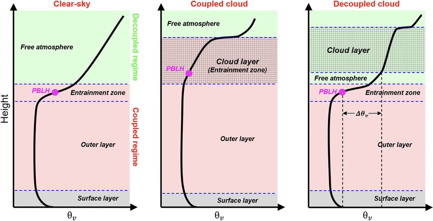
1454                                                 T. Su et al.: Methodology to determine the coupling of continental clouds

the determination methods of the PBL over land differ from          formance of the method is demonstrated in Sect. 4, and a
those over ocean (Garratt, 1994; Vogelezang and Holtslag,           summary is presented in Sect. 5.
1996). The concept of coupled and decoupled states is typ-
ically used to characterize marine stratocumulus clouds due
                                                                    2     Data descriptions
to their large-scale coverages (Nicholls, 1984). Since stra-
tocumulus only constitutes a relatively small portion of con-       2.1    Radiosonde
tinental clouds (Warren et al., 1986), we attempt to extend
the concept of coupling and decoupling to characterize low          RS launches took place at least four times per day at the
clouds over land. Due to the relatively complex thermody-           ARM SGP site, usually at 00:30, 06:30, 12:30, and 18:30
namics, the moisture conserved variables (e.g., total water         local time (LT). Holdridge et al. (2011) provide technical de-
mixing ratio and liquid potential temperature) may not be a         tails about the ARM RS (https://www.arm.gov/capabilities/
constant in the coupled sub-cloud layer (Driedonks, 1982;           instruments/sonde, last access: 2 December 2021). In this
Stull, 1988).                                                       study, we consistently use daylight saving time (coordinated
   Following parcel theory, the lifted condensation level           universal time −5 h) as local time throughout the year to
(LCL) has been used to diagnose a coupled cloud, based on           avoid inconsistencies between summer and winter. Besides
the distance between the LCL and the cloud base (e.g., Dong         the routine measurements, there are fewer but still consider-
et al., 2015; Glenn et al., 2020; Zheng and Rosenfeld, 2015;        able numbers of RS data obtained at other times of the day
Zheng et al., 2020). When potential temperature and humid-          (e.g., 09:30, 12:00, 13:00, 15:30, and 19:00 LT). These sup-
ity are uniformly distributed in the vertical, the LCL should       plemental RS samples at other times comprise ∼ 10 % of the
be consistent with the cloud base for coupled cases. However,       total number of cases. RS data from 06:30–19:00 LT are uti-
the cloud base for coupled cases can considerably differ from       lized in this study. The vertical resolution of RS data varies
the LCL over land because potential temperature and humid-          according to the rising rate of the balloon, but measurements
ity have large variabilities in the vertical scale within the PBL   are generally taken ∼ 10 m apart. We further vertically aver-
over land (Driedonks, 1982; Guo et al., 2016, 2021; Stull,          age the RS data to achieve a vertical resolution of 5 hPa.
1988; Su et al., 2017a). To address the limitation in the LCL          There are several methods to determine PBLH from RS-
method, we attempt to develop a remote sensing method to            measured potential temperature (θ ), pressure, and humid-
distinguish coupled and decoupled clouds over land.                 ity profiles. They include, among others, the parcel method
   Since the PBL height (PBLH) is the maximum height di-            (Holzworth, 1964), the gradient methods (Stull, 1988; Sei-
rectly influenced by surface fluxes, we consider coupling           del et al., 2010), and the Richardson number method (Vo-
with the PBL equivalent to coupling with the land surface.          gelezang and Holtslag, 1996). After examining the previ-
Thus, we use the PBLH as a critical parameter to diagnose           ous methods, Liu and Liang (2010) proposed a different ap-
the coupling between clouds and the land surface. The de-           proach to determine the PBLH that is valid under differ-
gree of coupling may thus be gauged in terms of quantitative        ent thermodynamic conditions. The robust performance was
differences between the cloud base and the PBL top. Such            demonstrated over the SGP site and in other major field cam-
differences can be determined in a height coordinate system         paign sites around the world (Liu and Liang, 2010). Thus,
or in a potential temperature coordinate system (Kasahara,          we adopted this method to calculate PBLH from RS data in
1974). For this purpose, ground-based lidar has great poten-        this study. By using the water vapor mixing ratio (WVMR),
tial because it can continuously track the development of the       the potential temperature is corrected as the virtual poten-
PBL (Demoz et al., 2006; Hageli et al., 2000; Sawyer and Li,        tial temperature, θv (θv = θ(1 + 0.61 WVMR)). The virtual
2013; Su et al., 2017b, 2018) and clouds (Clothiaux et al.,         potential temperature does not include a correction for the
2000; Platt et al., 1994; Zhao et al., 2014) at high temporal       liquid water content profile, as this is challenging to mea-
and vertical resolutions.                                           sure in many conditions. Therefore, the virtual potential tem-
   By jointly using lidar measurements and meteorological           perature is not conserved during moist convection. Since
data from the U.S. Department of Energy’s Atmospheric Ra-           we mainly focus on the sub-cloud atmosphere, this is not
diation Measurement (ARM) Southern Great Plains (SGP)               a serious problem. Moreover, for available datasets, we use
site (36.6◦ N, 97.48◦ W), we attempt to identify coupled and        scaled RS moisture profiles normalized by the total precip-
decoupled low clouds during the daytime. Unlike previous            itable water vapor derived from the microwave radiometer
studies that use the LCL or radiosonde (RS) data to diagnose        (https://www.arm.gov/capabilities/vaps/lssonde, last access:
coupled clouds (e.g., Dong et al., 2015; Zheng and Rosen-           2 December 2021, Revercomb et al., 2003).
feld, 2015), this study developed a lidar-based method to de-
termine the status of cloud coupling over land at a high tem-       2.2    Micropulse lidar (MPL) system
poral resolution.
   The paper is organized as follows. Section 2 describes the       MPL backscatter profiles were collected at the SGP site
measurements and data. Section 3 describes the new method-          from September 1998 to July 2019 with high continuity
ology in terms of the definition and implementation. The per-       (Campbell et al., 2002). Technical details and data avail-

Atmos. Chem. Phys., 22, 1453–1466, 2022                                              https://doi.org/10.5194/acp-22-1453-2022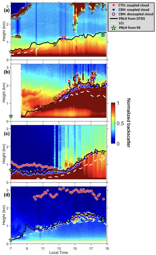
T. Su et al.: Methodology to determine the coupling of continental clouds 1455
ability can be found at the website https://www.arm.gov/ The outer layer and entrainment zone are turbulently cou-
capabilities/instruments/mpl, last access: 1 December 2021. pled with the surface and, thus, are considered as the coupled
The backscatter profiles have a vertical resolution of 30 m. regime. Meanwhile, the free atmosphere is considered as the
MPL signals have an initial temporal resolution of 10–30 s decoupled regime. Theoretically, θv is constant in the outer
and are averaged every 10 min for this study. Due to the layer and follows the wet adiabatic lapse rate in the cloud
inherent problem of lidar observations, there is a ∼ 0.2 km layer. Although the profiles of θv in the real atmosphere can
near-surface blind zone. Following the standard lidar-data largely differ from the idealized profiles, the relative position
processing, background subtraction, signal saturation and between the cloud layer and capping inversion of entrainment
overlapping, and after-pulse and range corrections are ap- zone is clear. For the coupled cases, the cloud base is below
plied to the raw MPL data (Campbell et al., 2002, 2003). the capping inversion of entrainment zone. For the decoupled
Questionable data are excluded based on the quality-control cases, the cloud base is above the capping inversion. Based
flags. on this feature, we can use the profiles of virtual potential
temperature (θv ) in the sub-cloud layer to determine the cou-
2.3 Cloud product
pling state of continental clouds. It should be noted that the
virtual potential temperature is not conserved in a moist adi-
The MPL can be used to detect cloud layers based on sig- abatic process and thus would decrease within a cloud layer.
nal gradients (Platt et al., 1994). Lidar-based methods are On the other hand, the liquid potential temperature remains
accurate for determining the cloud-base height (CBH) but a near-constant within the stratocumulus. Since we use the
may miss information about the cloud top due to the signal profiles of potential temperature in the sub-cloud layer to di-
saturation within an optically thick cloud (Clothiaux et al., agnose the cloud coupling, there is no difference in the iden-
2000). Under this condition, the cloud radar provides a bet- tification results by using the virtual potential temperature.
ter estimation of the cloud-top height (CTH). In this study, Following the previous studies (Jones et al., 2011; Dong
we directly use an existing quality-controlled cloud product, et al., 2015), we attempt to use the variations in the poten-
CLDTYPE/ARSCL (https://www.arm.gov/capabilities/vaps/ tial temperature within the sub-cloud layer to diagnose the
cldtype, last access: 1 December 2021), which combines in- cloud coupling. For determining a suitable threshold, we first
formation from the MPL, ceilometer, and cloud radar to de- look at several examples of profiles of θv and WVMR from
termine the vertical boundaries of clouds (ARM Data Cen- the RS (Fig. 2). If the CBH is lower than the PBLH, the
ter, 2021; Flynn et al., 2017). For the lowest cloud base, the cloud is affected by turbulence and buoyancy fluxes in the
best estimation from laser-based techniques (i.e., MPL and PBL, such as the cases shown in Fig. 2a. Note that the PBLH
ceilometer) is used. The original temporal resolution of the is not an absolute boundary limiting turbulence and buoy-
CLDTYPE/ARSCL product is 1 min, averaged to a 10 min ancy fluxes. Due to the overshooting of rising air parcels, we
temporal resolution. To avoid averaging jumps in signal be- use a range to screen the condition of coupled clouds. As
tween different clouds, a cloud is considered to be continu- shown in Fig. 2b, even when the CBH is slightly above the
ous if its base height varies less than 0.25 km between two PBLH, WVMR and θv are still relatively consistent between
consecutive profiles. the cloud layer and the PBL and show large step signals at
the cloud top.
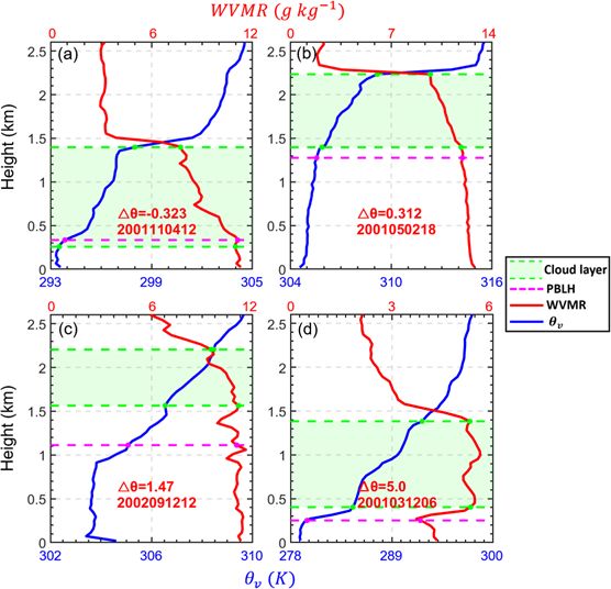
Figure 2c–d show a clear inversion layer between the cloud
3 Methodology
base and the PBL top, and the difference in θv between the
3.1 Definition of coupled and decoupled clouds based
CBH and the PBLH (1θv ) is relatively large. Such a notable
on thermodynamics
inversion layer prevents the buoyancy fluxes within the PBL
from reaching the cloud base, leading to the decoupling be-
The definition of the state of cloud–surface coupling over tween the cloud and the PBL. Overall, we consider 1θv as
land is a critical question. For marine stratocumulus, coupled the key factor to determine cloud coupling. In Fig. 2, 1θv for
clouds are identified when the liquid water potential tempera- coupled cases (a–c) is −0.32 and 0.31 K, respectively, and
ture varies less than a certain threshold (i.e., 0.5 K) below the 1θv for decoupled cases (d–e) is 1.47 and 5.0 K, respectively.
cloud base (Jones et al., 2011). We try to extend the concept Therefore, instead of giving a height range to limit the dif-
of coupling and decoupling to clouds over land. The PBL ferences between CBH and PBLH, we consider using the
over land is typically buoyancy driven and controlled by sur- differences in θv between CBH and PBLH to determine the
face fluxes during the daytime. We consider a cloud is in the threshold for distinguishing coupled and decoupled clouds.
coupled state when it strongly interacts with the buoyancy For convenience, we use 1θv to refer to the difference in θv
fluxes within the PBL. between the CBH and the PBLH (1θv = θvCBH −θvPBLH ). For
Figure 1 presents the idealized vertical profiles of vir- decoupled cases, the cloud base is above the capping inver-
tual potential temperature (θv ) under the clear sky, coupled sion of the entrainment zone. There is a notable inversion
cloud, and decoupled cloud. A superadiabatic surface layer in θv between PBL top and decoupled cloud base. Thus, we
exchanges the heat fluxes between the surface and PBL. identify the cases satisfying 1θv > δs as being in a decou-
https://doi.org/10.5194/acp-22-1453-2022 Atmos. Chem. Phys., 22, 1453–1466, 2022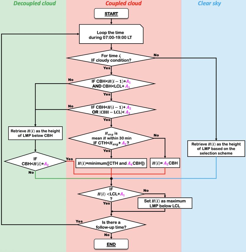
1456                                                    T. Su et al.: Methodology to determine the coupling of continental clouds

Figure 1. Idealized vertical profiles of virtual potential temperature (θv ) under the clear sky, coupled cloud, and decoupled cloud over land.
The surface layer, outer layer entrainment zone, and free atmosphere are divided by the dashed blue lines. The cloudy layer is marked as the
shaded area, and PBLH is marked as the pink point. Red and green zones indicate the coupled and decoupled regime, respectively. Elements
(e.g., turbulence, heat fluxes, cloud) in the coupled regime are directly affected by the PBL processes, while these elements are not directly
affected by the PBL processes in the decoupled regime. For the coupled cases, the cloud base is below the capping inversion of entrainment
zone. For the decoupled cases, the cloud base is above the capping inversion.

pled state. Correspondingly, we identify the cases satisfying             tions (Liu and Liang, 2010). Furthermore, we demonstrate
1θv < δs as being in a coupled state. We set the range of                 the probability density function (PDF) of 1θv for the low-
CBH to between 0 and 4 km and excluded cases of deep con-                 cloud cases. Coupled and decoupled clouds are classified by
vection (i.e., CBH < 4 km and CTH > 6.5 km). In the previ-                the threshold of δs (1 K). Through the development of PBL,
ous studies for marine clouds, the difference in the potential            boundary layer clouds frequently occur in the entrainment
temperature between the CBH and the near surface is used as               zone and form a coupled cloud–PBL system. For such cou-
the criterion (Jones et al., 2011; Dong et al., 2015). However,           pled systems, θv at cloud top and PBL top is highly consis-
we use the potential temperature at the PBL top instead of                tent for the majority of cases. Thus, the PDF of 1θv shows
the potential temperature near the surface. This change is due            significantly high values for the range of −2 to 0.5 K in the
to the relatively complex thermodynamic structure over the                coupled regime. Meanwhile, the PDF of 1θv is evenly dis-
land. The large variation in the potential temperature within             tributed in the decoupled regime. Since we only analyze low
the surface layer would notably affect the result. Hence, we              clouds, the PDF of 1θv slowly decreases when 1θv is above
use the potential temperature above the PBL top to replace                10 K.
those values near the surface.                                               Based on the variations in θv within the PBL, we set δs
   As the basic framework of PBL, the slab model assumes                  as 1 K. However, it should be noted that it is not an absolute
that θv is constant within the PBL (Wallace and Hobbs,                    value. A similar threshold of 0.5 K has been used for marine
2006). Under this assumption, δs can be set as 0. However,                stratocumulus (Jones et al., 2011; Dong et al., 2015). Com-
there are certain variations in θv within the PBL, which can              paring to the marine condition, θv shows greater variabilities
cause inversions with relatively small magnitudes between                 over land. Hence, the threshold is correspondingly larger. On
the cloud base and PBL top. Figure 3a presents the inversion              the other hand, since the threshold of 1 K is in the low PDF
strength in θv within PBL during the daytime. Specifically,               regime (Fig. 3b), the small changes in this value would not
inversions represent the layers with continuously increased               notably affect the identifications. Specifically, a 0.1 K differ-
structures of θv . For an inversion layer, the inversion strength         ence in δs will lead to a 0.5 % difference in the identification
is calculated as the differences in θv between the top and bot-           of coupled cloud.
tom of the layer. The inversions near the surface or across the              Similar to the previous studies (Jones et al., 2010; Dong et
PBL top are excluded. Besides the capping inversion and sur-              al., 2015; Zheng and Rosenfeld, 2015), we identified the cou-
face inversion, the inversion strength within PBL is typically            pled clouds as the thermodynamics coupling between surface
below 1 K. Therefore, we set δs as 1 K, which is the same                 and cloud base. However, it is an open question whether the
as the criterion for determining stable or convective condi-              entire cloud layer is coupled for coupled cases. It depends on

Atmos. Chem. Phys., 22, 1453–1466, 2022                                                      https://doi.org/10.5194/acp-22-1453-2022
T. Su et al.: Methodology to determine the coupling of continental clouds                                                           1457

Figure 2. Virtual potential temperature (θv , blue lines) and water
vapor mixing ratio (WVMR, red lines) profiles from radiosonde
(RS) over the Southern Great Plains site for different cases. The     Figure 3. (a) Blue bars represent the inversion strength of θv within
differences in virtual potential temperature between the cloud base   the PBL. The inversion strength is derived from the radiosonde
and the planetary boundary layer (PBL) top are expressed as           during daytime (08:00–19:00 LT). The inversions near the surface
1θv (θvCBH −θvPBLH ). The time of each radiosonde launch is marked    or across PBL top are excluded. The solid black line represents
in each panel as “YYYYMMDDHH”, where YYYY, MM, DD,                    the cumulative frequency. (b) Pink area represents the probabil-
and HH indicate the year, month, day, and local time, respec-         ity density function (PDF) of the differences in the virtual po-
tively. Green regions are cloud layers, and dashed green lines in-    tential temperature between cloud-base height (CBH) and PBLH
dicate their boundaries. The cloud layer is obtained from the CLD-    (1θv = θvCBH − θvPBLH ). By using a threshold of 1θv < δs (1 K),
TYPE/ARSCL data. PBLHs is derived from RS data and is marked          we can identify the coupled cloud regime.
as dashed pink lines.

whether the liquid water potential temperature is conserved           ment due to the coarse temporal resolution and drifting of the
within the cloud layer, which represents a moisture adiabatic         balloon. We thus further developed a lidar-based method to
process. This issue is closely related to the cloud types. In         identify the coupled states of clouds based on our new algo-
the cloud parameterizations, the entire stratocumulus layer           rithm for retrieving the PBLH that can better track the diurnal
is considered to be well-mixed, while the cumulus-capped              variations in PBLH than conventional lidar-based approaches
layer is usually partially mixed (Lock, 2000). For stratocu-          (Su et al., 2020). We adapted this algorithm for retrieving
mulus clouds, the entire cloud layer and PBL are typically            the PBLH and developed a new scheme to deal with cloudy
fully coupled with surface, when the cloud base is coupled            conditions. Following the original method (Su et al., 2020),
with surface. For the cumulus-capped PBL, the entire cloud            the rainy cases are eliminated in the quality-control process.
layer may not be completely coupled, despite the coupling             The principles behind the PBLH algorithm are stated next for
between cloud base and surface. The well-established pa-              completeness.
rameterizations are supported by many observational studies              Our new PBLH algorithm can retrieve the PBL variabil-
(e.g., Betts, 1986; Storer et al., 2015; Berkes et al., 2016; de      ity from the MPL under different thermodynamic stability
Roode and Wang. 2006; Ott et al., 2009).                              (thus named the DTDS algorithm) conditions, taking into
                                                                      account the vertical coherence and temporal continuity of
                                                                      the PBLH. First, we identify the local maximum positions
3.2     Lidar-based method to identify coupled and                    (LMPs; range: 0.25–4 km) in profiles of the wavelet co-
        decoupled clouds                                              variance transform function derived from lidar backscatter
3.2.1    Method description
                                                                      (Brooks, 2003). These LMPs are the potential positions of
                                                                      the PBLH. We can use the PBLH derived from morning RS
Given the rapid change in clouds over land, RS observations           soundings as the starting point. Without morning RS sound-
have limitations when it comes to tracking cloud develop-             ings, the algorithm can still work well, with the lowest LMPs

https://doi.org/10.5194/acp-22-1453-2022                                               Atmos. Chem. Phys., 22, 1453–1466, 2022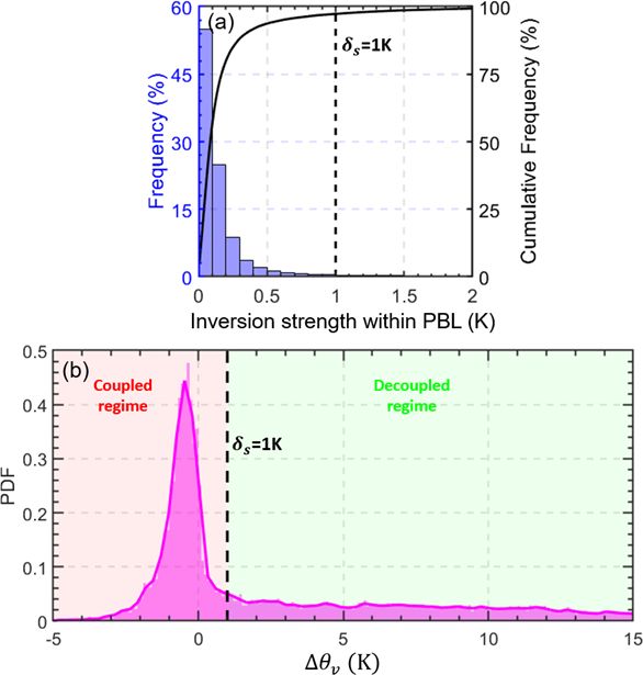
1458                                                   T. Su et al.: Methodology to determine the coupling of continental clouds

Table 1. List of parameters in the flowchart of DTDS (Fig. 4).

                                     Unit             Related       Value   Sensitivity        Sensitivity
                                                      factors               (coupled states)   (PBLH)
                              A1     km               LCL/PBLH        0.7   Low                Low
                              A2     km               PBLH            0.2   High               Low
                              A3     km               LCL            0.15   Low                Low
                              A4     dimensionless    CBH            1.35   Low                Low
                              A5     dimensionless    CBH             1.1   Low                High

selected as the starting point, which reduces by 0.02–0.05 the        with the LCL within 0.15 km (A3 ), and the CBH is less than
correlation coefficient between MPL-derived and RS-derived            [H (i−1)+0.7 km (A1 )], where H (i−1) represents the PBLH
PBLHs (Su et al., 2020).                                              at time (i − 1). This step further moves 17.8 % of the remain-
   To ensure good continuity, we select the closest LMP to            ing cases to the category of decoupled clouds.
the earlier position of the PBLH. Different stages of PBL de-            The LCL is calculated from surface meteorological data
velopment are considered. DTDS-derived PBLHs likely in-               (relative humidity, temperature, pressure) at the SGP site
crease during the growth stage and decrease during the de-            based on an exact expression (Romps, 2017). Specifically,
caying stage, but the algorithm is also able to identify de-          Romps (2017) proposed an exact, explicit, analytic expres-
creases during the growth stage or increases during the de-           sion for LCL as a function of surface meteorology. Compared
caying stage based on the selection scheme described by Su            to the previous approximate expressions, some of which may
et al. (2020). There are multiple step signals in the backscat-       have an uncertainty in the order of hundreds of meters, the
ter profiles when complex aerosol structures (e.g., the resid-        Romps expression can be considered as the precise value.
ual layer) are present, leading to multiple LMPs. Based on            The uncertainty of empirical vapor pressure data may lead to
temporal continuity, we select the appropriate LMP as the             a bias of ∼ 5 m (Romps, 2017), which may be neglected in
position of the PBL top. However, PBLH retrievals still suf-          the analyses.
fer from relatively low accuracies under stable conditions be-           After determining the coupling or decoupling state of a
cause of the weak vertical mixing and residual layer.                 cloud, we retrieve H (i) (i.e., PBLH at time i) based on the
   Clouds induce strong step signals in the lidar backscat-           cloud state. For decoupled cases, we use the same strategy
ter, further considerably affecting PBLH retrievals. Su et            for a clear sky to retrieve the PBLH. Based on the selection
al. (2020) only considered cases where the low cloud top              scheme in the DTDS algorithm, the LMP below the CBH
coincided with the previous PBL top, excluding other low-             is selected as H (i). For coupled cases, we jointly use CBH
cloud cases (> 60 % of all low-cloud cases). Here, we specif-         and CTH to determine PBLH. During the warm season, ac-
ically consider coupled and decoupled states of low clouds.           tive cumulus often occurs in the upper part of the PBL with
Due to the MPL’s ∼ 0.2 km blind zone, we only analyze                 strong surface heating, so the CBH can be generally regarded
the PBLH and CBH above 0.2 km. Figure 4 presents the                  as the PBLH (Stull, 1988; Wallace and Hobbs, 2006). Un-
flowchart describing the updated DTDS algorithm. In partic-           der this condition, the CBH coincides with the previous PBL
ular, we jointly use PBL development and the LCL to diag-             top. Therefore, if [CTH ≥ PBLH30 min + 0.2 km (A2 )], we
nose the states of coupling or decoupling. In ideal situations,       set H (i) = A5 CBH, where PBLH30 min is the average value
LCL, PBLH, and CBH are highly consistent with each other              of the PBLH within 30 min of the prior time i. Hence, A5
for coupled clouds. But for real conditions, we only require          would be a critical parameter for the PBLH estimation. On
that either the LCL or the PBLH coincides with the CBH for            the other hand, if [CTH < PBLH30 min + 0.2 km (A2 )], we
identifying coupled cases, with another parameter serving as          set H (i) equal to the minimum between CTH and the prod-
an additional constraint. Specifically, a coupled cloud needs         uct A4 × CBH. This step is designed for thin clouds or some
to occur within a certain range of LCL and the previous po-           stratiform clouds. In particular, A5 × CBH can be notably
sition of the PBL top.                                                larger than the CTH for a thin cloud. Under this situation,
   For the DTDS algorithm, five empirical parameters are              we tend to use CTH to denote the PBL top. This step has lit-
used, including A1 , A2 , A3 , A4 , and A5 . As listed in the Ta-     tle impact on the detection of surface–cloud coupling but can
ble 1, A1 –A5 are set as 0.7, 0.2, 0.15, 1.35, and 1.1, respec-       ensure that the CTH of the coupled cloud is always higher
tively. A cloud at time i is identified as being in the coupled       than the retrieved PBLH to fit the real situation.
state if the CBH is less than [H (i − 1) + 0.2 km (A2 )] and             After retrieving H (i), we consider that the cloud above
[LCL +0.7 km (A1 )]. This step moves 39.5 % of low-cloud              the PBLH is still coupled if [CBH < H (i) + 0.2 km (A2 )].
cases to the category of decoupled clouds. A cloud is also            Moreover, we added an upper limit for all PBLH retrievals.
considered to be in a coupled state if the CBH is coincident          If [H (i) > LCL + 0.7 km (A1 )], we adjust H (i) as the max-

Atmos. Chem. Phys., 22, 1453–1466, 2022                                                 https://doi.org/10.5194/acp-22-1453-2022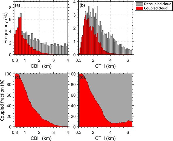
T. Su et al.: Methodology to determine the coupling of continental clouds                                                                 1459

Figure 4. The flowchart of the updated DTDS algorithm. In this diagram, H (i) is the retrieved planetary boundary layer height (PBLH)
at time i. CBH and CTH represent the base and top heights, respectively, of the lowest cloud at time i. The PBLH part for selecting the
suitable local maximum position (LMP) follows Su et al. (2020), and a detailed scheme for identifying a coupled cloud is added to the DTDS
algorithm. LCL stands for lifted condensation level. Five empirical parameters (A1 , A2 , A3 , A4 , and A5 ) are set as 0.7, 0.2, 0.15, 1.35, and
1.1, respectively.

imum LMP below the LCL. The new DTDS method com-                           pacts of variations in these parameters on the retrievals of
bines lidar measurements and surface meteorological obser-                 cloud coupling and PBLH will be discussed in this section.
vations and can simultaneously retrieve the PBLH and cloud                     Note that we used the CTH and A4 × CBH as the upper
states.                                                                    limits for PBLH retrievals in the DTDS algorithm. For cou-
                                                                           pled cases, these two limits are generally close to or above the
                                                                           position of the PBL top. Only 2 % (3 %) of total cases meet
3.2.2   Selection of empirical parameters                                  the condition that the RS-derived PBLH is 0.25 km higher
                                                                           than the CTH (A4 × CBH). Section 4 presents the detailed
The states of coupling and decoupling are diagnostic param-                relationships between CBH, CTH, and PBLH. In the DTDS
eters rather than explicit expressions. Similar to the other               method, CTH serves as the upper limit for PBLH under the
methods for retrieving PBLH (e.g., Brooks, 2003; Liu and                   condition of coupled shallow cumulus.
Liang, 2010), multiple empirical parameters are used to de-                    Similar to previous studies, we can also use the LCL as
termine PBLH. Table 1 lists the five empirical parameters in               the standard to identify coupled clouds (Dong et al., 2015;
the algorithm. These parameters are related with three fac-                Zheng and Rosenfeld, 2015). We assume a cloud is coupled
tors, including LCL, PBLH, and CBH. The sensitivity to the                 if |CBH-LCL| < 1h. By using ∼ 7500 RS profiles, the cloud
selection of these parameters is presented. The detailed im-               coupling state derived from the virtual potential temperature

https://doi.org/10.5194/acp-22-1453-2022                                                    Atmos. Chem. Phys., 22, 1453–1466, 2022
1460 T. Su et al.: Methodology to determine the coupling of continental clouds
Figure 5. Commission errors and omission errors of coupled cloud
identifications (a) for different criteria for the lifted condensa-
tion level (LCL) and (b) for different criteria for the planetary
boundary layer height (PBLH). “Criteria for LCL” means coupled Figure 6. Commission errors (red line) and omission errors (blue
clouds are identified if |CBH − LCL| < criteria for LCL. Similarly, line) of coupled cloud identifications for selecting different values
“Criteria for RS PBLH” means coupled clouds are identified if of empirical parameters (A1 , A2 , A3 , A4 , A5 ) in the DTDS algo-
CBH − RS PBLH < criteria for RS PBLH. The dashed red and blue rithm. Dashed black lines indicate the default values. For each test,
lines indicate the commission and omission errors, respectively, for one parameter is variable, while other parameters are set as default
the DTDS algorithm. CBH stands for cloud-base height, and RS values. For identifications of cloud coupling, A2 is the critical pa-
stands for radiosonde. By using ∼ 7500 RS profiles, the cloud cou- rameter.
pling state derived from the virtual potential temperature method
(Sect. 3.1) is considered as the ground truth for evaluation.
Moreover, we test the sensitivity of selecting these empir-
ical parameters. Figure 6 presents the commission errors and
method (Sect. 3.1) is considered as the ground truth for eval-
omission errors in the identifications of coupled clouds for
uation. Figure 5a shows the commission errors and omission
selecting different values of empirical parameters. Among
errors for different criteria. Here, the commission error is cal-
these parameters, A2 is the critical one, which would notably
culated as the percentage of decoupled clouds misidentified
affect the identification results. In general, A2 determines the
as coupled clouds. The commission error can also be called
maximum differences between PBLH and CBH for coupled
a “false positive”, as the former is a common term for de-
cases. If [CBH − PBLH > A2 ], we consider the cloud is un-
scribing the nature of an error in identification. The omission
der the decoupled state. Thus, the identification method is
error is calculated as the percentage of coupled clouds that
quite sensitive to A2 . Selecting a low value of A2 would ne-
have not been identified under this criterion. By using the
glect many coupled cases, which leads to a high omission er-
LCL, we can obtain a relatively low commission error if the
ror. Meanwhile, selecting a high value of A2 would misclas-
criterion is less than 0.15 km and a relatively low omission
sify many coupled cases, which leads to a high commission
error if the criterion is greater than 0.7 km. Thus, we set A1
error. After a trail and error, A2 is set as 0.2 km to balance
and A3 as 0.7 and 0.15 in the DTDS method to exclude and
the omission and commission errors. The selections for other
to select cases of coupled clouds. We can also use the RS-
parameters are not sensitive for the coupled cloud identifica-
derived PBLH as the criterion (Fig. 5b).
tions. We can choose them from a reasonable range.
Despite the coarse temporal resolution, the RS-derived
As a by-product of this method, we also pay attention
PBLH can be a good criterion to use to distinguish between
to the PBLH retrievals under cloudy conditions. Figure 7
coupling and decoupling. If we consider a coupled cloud
presents the mean absolute biases and correlation coefficients
as a cloud where CBH < RS-derived PBLH + 0.2 km, both
between PBLH derived from lidar and radiosonde for select-
commission and omission errors are ∼ 5 %. Therefore, we
ing different values of empirical parameters. To match the
primarily use [PBLH + 0.2 km (A2 )] in the DTDS method
scope of this study, we only analyze the low-cloud condi-
to identify coupled and decoupled regimes. As cloud can
tions. For retrieving PBLH under cloudy conditions, A2 is the
considerably affect with lidar backscattering and generate
critical parameter. The variations in correlation coefficients
large signal variations, we jointly use lidar backscattering,
under different values of empirical parameters are small with
the previous position of PBL top, and LCL to determine the
a range of 0.81–0.82. However, the absolute biases can con-
surface–cloud coupling and PBLH. In particular, the LCL
siderably differ under different values of A5 . In general, A5
constraint in the algorithm notably reduces the absolute bi-
represents the ratio between CBH and PBLH under coupled
ases in PBLH retrievals under cloudy conditions by 9.3 %.
conditions. If A5 is above 1.1, PBLH retrievals under cloudy
conditions are overestimated. We set A5 as 1.1 to achieve a
Atmos. Chem. Phys., 22, 1453–1466, 2022 https://doi.org/10.5194/acp-22-1453-2022T. Su et al.: Methodology to determine the coupling of continental clouds 1461
Figure 7. Red lines indicate the mean absolute biases between
PBLH derived from lidar and radiosonde for selecting different val-
ues of empirical parameters (A1 , A2 , A3 , A4 , A5 ) in the DTDS
algorithm. Here, we only analyze the low-cloud cases. Blue lines in-
dicate the corresponding correlation coefficients between PBLH de-
rived from lidar and radiosonde. Dashed black lines indicate the de-
fault values. For each test, one parameter is variable, while other pa-
rameters are set as default values. For PBLH retrievals under cloudy
conditions, A5 is the critical parameter.
relatively low bias and a relatively high correlation coeffi-
cient at the same time. For other parameters, the selections
from reasonable ranges would not notably affect the PBLH
retrievals.
In short, selections of these empirical parameters are based
on the overall relationship between cloud and PBL under the
coupled and decoupled states. In our method, the selection of
Figure 8. Daily backscatter profiles: (a) short-lived coupled cloud,
A2 is critical for the identifications of coupled clouds, while
(b) developed coupled cloud, (c) daylong coupled cloud, and (d) ac-
the selection of A5 is critical for the PBLH retrievals under
tive coupled cloud. Backscatter is normalized to a range of 0–
cloudy conditions. The selections of other parameters are not 1 in arbitrary units. Red dots and blue dots indicate cloud-top
sensitive. heights (CTHs) and cloud-base heights (CBHs) of coupled clouds.
Grey dots mark CBHs for decoupled clouds. Black lines and green
stars mark the planetary boundary layer height (PBLH) retrieved
4 Results from the DTDS algorithm and from radiosonde (RS) soundings, re-
spectively. Dashed white lines represent lifted condensation levels
Figure 8 illustrates four examples of PBLH retrievals and (LCLs).
cloud states derived from the DTDS algorithm for 27 Octo-
ber 2011, 31 July 2002, 19 March 2000, and 1 May 2012.
Figure 8a depicts coupled shallow cumulus occurring at case of an active coupled cloud, which is generally associ-
noontime at the PBL top. With a weak surface flux of ated with a large amount of convective available potential
∼ 200 W m−2 , this shallow cumulus cloud appeared for less energy. Even though coupled clouds can differ in appearance
than an hour. Figure 8b shows a developed coupled cumulus and variability throughout the day, the common feature is
cloud. With a strong surface flux of ∼ 500 W m−2 , this cou- the coherent variation between the cloud base and the PBL
pled cloud continuously developed during the daytime. Fig- top. The LCL is a relevant parameter and can differ from the
ure 8c presents the case of a daylong coupled cloud. After PBLH and the CBH for some coupled cases (e.g., Fig. 8b–c).
the passage of a frontal system that day, stratocumulus oc- The identification accuracy, or disparity between different
curred during the morning with a cloud thickness of 0.5 km. methods, is evaluated in terms of the selected criteria, for
Through the development of the PBL, the thick stratocumu- which the identification method based on 1θv is regarded as
lus cloud was broken up by the strong turbulences, trans- the “truth”, as described in Sect. 3.1. Hereafter, all results are
forming into shallow cumulus clouds. Figure 8d shows the analyzed for the period of 10:00–19:00 LT, so early-morning
https://doi.org/10.5194/acp-22-1453-2022 Atmos. Chem. Phys., 22, 1453–1466, 20221462 T. Su et al.: Methodology to determine the coupling of continental clouds
data are not used. The commission error is 10.1 %, and the
omission error is 6.8 % for the DTDS method. Note that
lidar-based PBLH methods generally suffer from relatively
low accuracy under stable atmospheric conditions. Follow-
ing Liu and Liang (2010), we identified stable PBLs from
RS measurements. Since coupled clouds are driven by rela-
tively strong buoyancy fluxes, only 1 % of total cases of cou-
pled clouds occurred under stable PBL conditions during the
study period (07:00–19:00 LT). Therefore, the relatively low
accuracy for stable PBLs is not a major problem in this study.
Figure 5 also compares the accuracy between the DTDS
and LCL methods. Based on the LCL alone, we cannot
choose an appropriate criterion to achieve a lower commis-
sion error and omission error simultaneously. Thus, we do
not use the LCL as the single standard to detect the coupling
and decoupling of low clouds in our study. As diagnostic pa-
rameters, different methods inevitably produce different re-
sults regarding coupling and decoupling. Although we con-
Figure 9. The height-dependent occurrence frequencies of (a) the
sider the method based on 1θv as the standard, it still suffers cloud-base height (CBH) and (b) the cloud-top height (CTH) for
from uncertainties arising from balloon drifting. From this coupled clouds (red bars) and decoupled clouds (grey bars). The
perspective, it is hard to conclude which method is the best. relative occurrence frequencies of (c) the CBH and (d) the CTH for
Since it determines the PBLH based on aerosol backscatter- coupled clouds (red area) and decoupled clouds (grey area).
ing, the lidar-based method may be more representative of
the coupling between a cloud and the aerosol layer near the
surface when clear skies occur, at least during a short window ter or lidar still bear some uncertainties, which can poten-
of time. tially lead to a mean bias of 0.1 km (Silber et al., 2018). In
Figure 9a–b present the occurrence frequencies of the our method, a systematic increase of 0.1 km in the CBH can
CBH and the CTH at different heights. Despite the same vari- lead to an increase of 2.1 % in omission errors and a decrease
ation ranges, clouds are mostly coupled if the CBH is lower of 1 % in commission errors.
than 1 km, while decoupled clouds dominate if the CBH is After identifying the coupling state of clouds, it is feasi-
higher than 3 km. Figure 9c–d show the changes in the cou- ble to retrieve the PBLH under cloudy conditions. In par-
pled fraction (ratio of coupled cases to total cases) with dif- ticular, the DTDS-derived PBLH needs to resort to the
ferent CBHs and CTHs. The coupled fraction is about 90 % cloud position for coupled cloud cases. For decoupled cloud
if the CBH is lower than 1 km and decreases to 2 % for CBHs cases, on the other hand, the PBLH below clouds is sought
above 3 km. Although the CBHs for coupled cases are gen- to avoid cloud interference. For coupled clouds, DTDS-
erally less than 3 km, CTHs for coupled cases can be much derived PBLHs show a strong correlation with RS-derived
higher. Coupled clouds still account for around 10 % of the PBLHs with a correlation coefficient (R) of ∼ 0.9 (Fig. 10d).
cases with CTHs above 6 km. For decoupled cases, the correlation between DTDS-derived
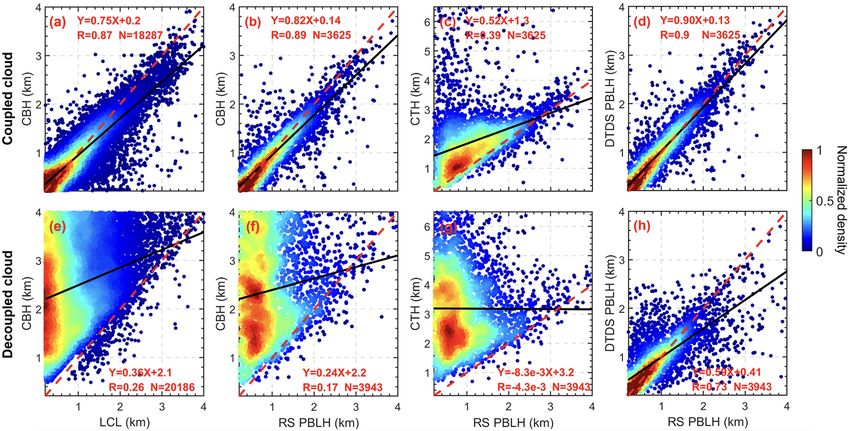
Figure 10 shows scatter plots between CBH, CTH, PBLH, PBLHs and RS-derived PBLHs is generally good (R = 0.73)
and LCL for coupled and decoupled clouds. For coupled but worse than the correlation for coupled cases (Fig. 10h).
clouds, there is a generally strong correlation between CBH, As pointed out in previous studies (Chu et al., 2019; Hageli
LCL, and PBLH, contrary to the weak relationships of et al., 2000; Lewis et al., 2013; Su et al., 2017b), it has been a
decoupled cases. The relationship between CTH and RS- persistent problem to retrieve the PBLH under cloudy condi-
derived PBLH is complicated. For shallow cumulus clouds, tions since the strong backscattering and step signals from
their tops can be considered as PBL tops for the coupled cloud interference would be excluded to avoid interfering
state, while the cloud top is considerably above the position with the retrievals. The PBLH determined by our method un-
of the PBL top for active cumulus clouds. We also note that der a cloudy condition is much more reasonable. Moreover,
the accuracy of CTH retrievals is generally lower than the due to the different definitions of the PBLH and aerosol strat-
accuracy of CBH retrievals (Clothiaux et al., 2000). As CTH ification within the PBL, there are always considerable dif-
is not a criterion for cloud coupling, the accuracy of CTH ferences between lidar- and RS-derived PBLHs, which can-
would not affect the identification of coupled cloud but may not be eliminated by a specific algorithm (Chu et al., 2019;
affect the PBLH retrievals for the coupled cloud cases. Mean- Su et al., 2020).
while, despite the laser-based detection of CBH being con-
sidered the standard method (Platt et al., 1994; Clothiaux et
al., 2000; Lim et al., 2019), the CBH retrievals from ceilome-
Atmos. Chem. Phys., 22, 1453–1466, 2022 https://doi.org/10.5194/acp-22-1453-2022T. Su et al.: Methodology to determine the coupling of continental clouds 1463
Figure 10. The relationships between (a) LCL and CBH, (b) CBH and RS-derived PBLH, (c) CTH and RS-derived PBLH for coupled
clouds, and (d) DTDS-derived PBLH and RS-derived PBLH. Panels (e)–(h) are similar to panels (a)–(d) but for decoupled clouds. Black
lines represent the linear regressions. The linear fitting functions, correlation coefficients (R), and sampling numbers (N) are given in each
panel.
5 Summary changes in the PBLH and buoyancy, the decoupled clouds
and the PBLH are weakly related. Due to their different re-
lationships with the PBL, a robust differentiation between
In this study, we proposed a novel method for distinguish- the coupled and decoupled low clouds is critical for fur-
ing between coupled and decoupled low clouds over land. ther investigating the coupled land–atmosphere system and
Based on the understanding of PBL processes and quantita- aerosol–cloud interactions. Our methodology paves a solid
tive analyses, we developed a lidar-based method (DTDS) to ground for such pursuits.
identify the coupling state of low clouds over the SGP site.
In practice, we identified a coupled cloud when the position
of the cloud base was generally close to or lower than the Data availability. All these datasets are publicly available at the
previous position of the PBL top, with the LCL serving as an ARM archive https://adc.arm.gov/discovery/#/results/site_code::
additional restriction. Compared to using the LCL alone, the sgp (ARM Data Center, 2021). The products developed in this
coupled states identified by the DTDS method show better study, i.e., cloud states and the PBLH, are currently available upon
consistency with the results derived from radiosondes, with request from the lead author (tianning@umd.edu) and are expected
about 10 % differences between the lidar-based retrievals and to be added to the ARM archive in the near future.
radiosonde results.
Not only the coupled state but also the PBLH under cloudy
conditions is retrieved by the method. A long-lasting prob- Author contributions. TS, YZ, and ZL conceptualized this study.
lem with lidar retrieval of PBLH is either incapability of re- TS carried out the analysis, with comments from other co-authors.
trieval or large uncertainties induced by the occurrence of TS, YZ, and ZL interpreted the data and wrote the manuscript.
low clouds (e.g., Chu et al., 2019; Hageli et al., 2000; Lewis
et al., 2013); we address this issue by separately consider-
Competing interests. The contact author has declared that nei-
ing the coupled and decoupled state of low clouds. Specifi-
ther they nor their co-authors have any competing interests.
cally, in coupled conditions, the position of the coupled cloud
serves as a good reference for identifying the PBLH. In de-
coupled conditions, the large backscatter and step signals Disclaimer. Publisher’s note: Copernicus Publications remains
from clouds would be excluded to avoid interfering with the neutral with regard to jurisdictional claims in published maps and
retrievals. With our method, cloudy conditions are well han- institutional affiliations.
dled.
With the new method, we study the difference of cloud–
PBL interactions in coupled and decoupled conditions. In
contrast to the sensitive responses of coupled clouds to
https://doi.org/10.5194/acp-22-1453-2022 Atmos. Chem. Phys., 22, 1453–1466, 20221464 T. Su et al.: Methodology to determine the coupling of continental clouds
Acknowledgements. We acknowledge the provision of ra- Clothiaux, E. E., Ackerman, T. P., Mace, G. G., Moran, K. P.,
diosonde, MPL data, surface meteorological data, and cloud prod- Marchand, R. T., Miller, M. A., and Martner, B. E.: Objective
ucts by the U.S. Department of Energy’s ARM program. We thank determination of cloud heights and radar reflectivities using a
the two anonymous reviewers for their comments. combination of active remote sensors at the ARM CART sites,
J. Appl. Meteorol., 39, 645–665, https://doi.org/10.1175/1520-
0450(2000)0392.0.CO;2, 2000.
Financial support. This research has been supported by the U.S. Demoz, B., Flamant, C., Weckwerth, T., Whiteman, D., Evans, K.,
Department of Energy (grant no. DE-SC0018996) and the National Fabry, F., Di Girolamo, P., Miller, D., Geerts, B., Brown, W.,
Science Foundation (grant nos. AGS2126098 and AGS1837811). Schwemmer, G., Gentry, B., Feltz, W., and Wang, Z.: The dryline
on 22 May 2002 during IHOP_ 2002: convective-scale measure-
ments at the profiling site, Mon. Weather Rev., 134, 294–310,
Review statement. This paper was edited by Yun Qian and re- https://doi.org/10.1175/MWR3054.1, 2006.
viewed by Xiquan Dong and two anonymous referees. de Roode, S. R. and Wang, Q.: Do stratocumulus clouds detrain?
FIRE I data revisited, Bound.-Lay. Meteorol., 122, 479–491,
2007.
Dong, X., Schwantes, A. C., Xi, B., and Wu, P.: Inves-
References tigation of the marine boundary layer cloud and CCN
properties under coupled and decoupled conditions over
ARM Data Center: Field Campaign Data Products, available at: the Azores, J. Geophys. Res.-Atmos., 120, 6179–6191,
https://adc.arm.gov/discovery/#/results/site_code::sgp, last ac- https://doi.org/10.1002/2014JD022939, 2015.
cess: 1 December 2021. Driedonks, A. G. M.: Models and observations of the growth of the
Berkes, F., Hoor, P., Bozem, H., Kunkel, D., Sprenger, M., and atmospheric boundary layer, Bound.-Lay. Meteorol., 23, 283–
Henne, S.: Airborne observation of mixing across the entrain- 306, https://doi.org/10.1007/BF00121117, 1982.
ment zone during PARADE 2011, Atmos. Chem. Phys., 16, Ek, M. B. and Holtslag, A. A. M.: Influence of soil mois-
6011–6025, https://doi.org/10.5194/acp-16-6011-2016, 2016. ture on boundary layer cloud development, J. Hy-
Betts, A. K.: Land-surface-atmosphere coupling in observa- drometeorol., 5, 86–99, https://doi.org/10.1175/1525-
tions and models, J. Adv. Model. Earth Syst., 1, 18 pp., 7541(2004)0052.0.CO;2, 2004.
https://doi.org/10.3894/JAMES.2009.1.4, 2009. Flynn, D., Shi, Y., Lim, K., and Riihimaki, L.: Cloud
Bretherton, C. S. and Wyant, M. C.: Moisture trans- Type Classification (cldtype) Value-Added Product, edited
port, lower-tropospheric stability, and decou- by: Stafford, R., ARM Research Facility, DOE/SC-ARM-
pling of cloud-topped boundary layers, J. Atmos. TR-200, available at: https://www.arm.gov/publications/tech_
Sci., 54, 148–167, https://doi.org/10.1175/1520- reports/doe-sc-arm-tr-200.pdf (last access: 2 December 2021),
0469(1997)0542.0.CO;2, 1997. 2017.
Brooks, I. M.: Finding boundary layer top: application of a wavelet Garratt, J. R.: Review: the atmospheric boundary layer, Earth-Sci.
covariance transform to lidar backscatter profiles, J. Atmos. Rev., 37, 89–134, https://doi.org/10.1016/0012-8252(94)90026-
Ocean. Technol., 20, 1092–1105, https://doi.org/10.1175/1520- 4, 1994.
0426(2003)0202.0.CO;2, 2003. Glenn, I. B., Feingold, G., Gristey, J. J., and Yamaguchi, T.: Quan-
Campbell, J. R., Hlavka, D. L., Welton, E. J., Flynn, C. tification of the radiative effect of aerosol-cloud-interactions in
J., Turner, D. D., Spinhirne, J. D., Scott III, V. S., and shallow continental cumulus clouds, J. Atmos. Sci., 77, 2905–
Hwang, I. H.: Full-time, eye-safe cloud and aerosol li- 2920, https://doi.org/10.1175/JAS-D-19-0269.1, 2020.
dar observation at atmospheric radiation measurement pro- Golaz, J. C., Larson, V. E., and Cotton, W. R.: A PDF-based model
gram sites: instruments and data processing, J. Atmos. for boundary layer clouds, Part I: Method and model description,
Ocean. Technol., 19, 431–442, https://doi.org/10.1175/1520- J. Atmos. Sci., 59, 3540–3551, https://doi.org/10.1175/1520-
0426(2002)0192.0.CO;2, 2002. 0469(2002)0592.0.CO;2, 2002.
Campbell, J. R., Welton, E. J., Spinhirne, J. D., Ji, Q., Tsay, Guo, J., Miao, Y., Zhang, Y., Liu, H., Li, Z., Zhang, W., He, J., Lou,
S. C., Piketh, S. J., Barenbrug, M., and Holben, B. N.: Mi- M., Yan, Y., Bian, L., and Zhai, P.: The climatology of plan-
cropulse lidar observations of tropospheric aerosols over north- etary boundary layer height in China derived from radiosonde
eastern South Africa during the ARREX and SAFARI 2000 and reanalysis data, Atmos. Chem. Phys., 16, 13309–13319,
dry season experiments, J. Geophys. Res.-Atmos., 108, 8497, https://doi.org/10.5194/acp-16-13309-2016, 2016.
https://doi.org/10.1029/2002JD002563, 2003. Guo, J., Zhang, J., Yang, K., Liao, H., Zhang, S., Huang, K., Lv,
Cheruy, F., Dufresne, J. L., Hourdin, F., and Ducharne, A.: Role Y., Shao, J., Yu, T., Tong, B., Li, J., Su, T., Yim, S. H. L., Stof-
of clouds and land-atmosphere coupling in midlatitude conti- felen, A., Zhai, P., and Xu, X.: Investigation of near-global day-
nental summer warm biases and climate change amplification time boundary layer height using high-resolution radiosondes:
in CMIP5 simulations, Geophys. Res. Lett., 41, 6493–6500, first results and comparison with ERA5, MERRA-2, JRA-55,
https://doi.org/10.1002/2014GL061145, 2014. and NCEP-2 reanalyses, Atmos. Chem. Phys., 21, 17079–17097,
Chu, Y., Li, J., Li, C., Tan, W., Su, T., and Li, J.: Seasonal and https://doi.org/10.5194/acp-21-17079-2021, 2021.
diurnal variability of planetary boundary layer height in Bei- Hageli, P., Steyn, D. G., and Strawbridge, K. B.: Spatial
jing: intercomparison between MPL and WRF results, Atmos. and temporal variability of mixed-layer depth and entrain-
Res., 227, 1–13, https://doi.org/10.1016/j.atmosres.2019.04.017,
2019.
Atmos. Chem. Phys., 22, 1453–1466, 2022 https://doi.org/10.5194/acp-22-1453-2022T. Su et al.: Methodology to determine the coupling of continental clouds 1465 ment zone thickness, Bound.-Lay. Meteorol., 97, 47–71, Romps, D. M.: Exact expression for the lifting condensation level, J. https://doi.org/10.1023/A:1002790424133, 2000. Atmos. Sci., 74, 3891–3900, https://doi.org/10.1175/JAS-D-17- Holdridge, D., Ritsche, M., Prell, J., and Coulter, R.: Balloon- 0102.1, 2017. borne sounding system (SONDE) handbook, ARM Data Center, Santanello, J. A., Dirmeyer, P. A., Ferguson, C. R., Findell, K. available at: https://www.arm.gov/capabilities/instruments/sonde L., Tawfik, A. B., Berg, A., Ek, M., Gentine, P., Guillod, B. (last access: 2 December 2021), 2011. P., van Heerwaarden, C., Roundy, J., and Wulfmeyer, V.: Land- Holzworth, G. C.: Estimates of mean maximum mix- atmosphere interactions: the LoCo perspective, Bull. Am. Mete- ing depths in the contiguous United States, Mon. orol. Soc., 99, 1253–1272, https://doi.org/10.1175/BAMS-D-17- Weather Rev., 92, 235–242, https://doi.org/10.1175/1520- 0001.1, 2018. 0493(1964)0922.3.co;2, 1964. Sawyer, V. and Li, Z. Q.: Detection, variations and intercompari- Jones, C. R., Bretherton, C. S., and Leon, D.: Coupled vs. decou- son of the planetary boundary layer depth from radiosonde, li- pled boundary layers in VOCALS-REx, Atmos. Chem. Phys., 11, dar and infrared spectrometer, Atmos. Environ., 79, 518–528, 7143–7153, https://doi.org/10.5194/acp-11-7143-2011, 2011. https://doi.org/10.1016/j.atmosenv.2013.07.019, 2013. Kasahara, A.: Various vertical coordinate systems used Seidel, D. J., Ao, C. O., and Li, K.: Estimating climatological plane- for numerical weather prediction, Mon. Weather tary boundary layer heights from radiosonde observations: Com- Rev., 102, 509–522, https://doi.org/10.1175/1520- parison of methods and uncertainty analysis, J. Geophys. Res.- 0493(1974)1022.0.CO;2, 1974. Atmos., 115 D16113, https://doi.org/10.1029/2009JD013680, Lewis, J. R., Welton, E. J., Molod, A. M., and Joseph, 2010. E.: Improved boundary layer depth retrievals from Silber, I., Verlinde, J., Eloranta, E. W., Flynn, C. J., and Flynn, D. MPLNET, J. Geophys. Res.-Atmos., 118, 9870–9879, M.: Polar liquid cloud base detection algorithms for high spec- https://doi.org/10.1002/jgrd.50570, 2013. tral resolution or micropulse lidar data, J. Geophys. Res.-Atmos., Lim, K. S. S., Riihimaki, L. D., Shi, Y., Flynn, D., Kleiss, J. M., 123, 4310–4322, https://doi.org/10.1029/2017JD027840, 2018. Berg, L. K., Gustafson, W. I., Zhang, Y., and Johnson, K. L.: Storer, R. L., Griffin, B. M., Höft, J., Weber, J. K., Raut, E., Lar- Long-term retrievals of cloud type and fair-weather shallow cu- son, V. E., Wang, M., and Rasch, P. J.: Parameterizing deep con- mulus events at the ARM SGP site, J. Atmos. Ocean. Technol., vection using the assumed probability density function method, 36, 2031–2043, 2019. Geosci. Model Dev., 8, 1–19, https://doi.org/10.5194/gmd-8-1- Liu, S. Y. and Liang, X. Z.: Observed diurnal cycle climatology 2015, 2015. of planetary boundary layer height, J. Clim., 23, 5790–5809, Stull, R. B.: An Introduction to Boundary Layer Meteorol- https://doi.org/10.1175/2010JCLI3552.1, 2010. ogy, Springer Science & Business Media, the Netherlands, Lock, A. P., Brown, A. R., Bush, M. R., Martin, G. M., and Smith, https://doi.org/10.1007/978-94-009-3027-8, 1988. R. N. B.: A new boundary layer mixing scheme, Part I: Scheme Su, T., Li, J., Li, J., Li, C., Chu, Y., Zhao, Y., Guo, J., Yu, description and single-column model tests, Mon. Eeather Rev., Y., and Wang, L.: The evolution of springtime water vapor 128, 3187–3199, 2000. over Beijing observed by a high dynamic Raman lidar sys- Nicholls, S.: The dynamics of stratocumulus: aircraft observations tem: case studies, IEEE J. Sel. Top. Appl., 10, 1715–1726, and comparisons with a mixed layer model, Q. J. Roy. Meteor. https://doi.org/10.1109/JSTARS.2017.2653811, 2017a. Soc., 110, 783–820, https://doi.org/10.1002/qj.49711046603, Su, T., Li, J., Li, C., Xiang, P., Lau, A.K.H., Guo, J., Yang, 1984. D., and Miao, Y.: An intercomparison of long-term plan- Ott, L. E., Bacmeister, J., Pawson, S., Pickering, K., Stenchikov, etary boundary layer heights retrieved from CALIPSO, G., Suarez, M., Huntrieser, H., Loewenstein, M., Lopez, J., and ground-based lidar, and radiosonde measurements over Xueref-Remy, I.: Analysis of convective transport and parameter Hong Kong, J. Geophys. Res.-Atmos., 122, 3929–3943, sensitivity in a single column version of the Goddard earth ob- https://doi.org/10.1002/2016JD025937, 2017b. servation system, version 5, general circulation model, J. Atmos. Su, T., Li, Z., and Kahn, R.: Relationships between the plan- Sci., 66, 627–646, 2009. etary boundary layer height and surface pollutants derived Platt, C. M., Young, S. A., Carswell, A. I., Pal, S. R., Mc- from lidar observations over China: regional pattern and in- Cormick, M. P., Winker, D. M., DelGuasta, M., Stefanutti, L., fluencing factors, Atmos. Chem. Phys., 18, 15921–15935, Eberhard, W. L., Hardesty, M., Flamant, P. H., Valentin, R., https://doi.org/10.5194/acp-18-15921-2018, 2018. Forgan, B., Gimmestad, G. G., Jäger, H., Khmelevtsov, S. S., Su, T., Li, Z., and Kahn, R.: A new method to retrieve the diurnal Kolev, I., Kaprieolev, B., Lu, D., Sassen, K., Shamanaev, V. S., variability of planetary boundary layer height from lidar under Uchino, O., Mizuno, Y., Wandinger, U., Weitkamp, C., Ans- different thermodynamic stability conditions, Remote Sens. En- mann, A., and Woolridge, C.: The Experimental Cloud LIdar viron., 237, 111519, https://doi.org/10.1016/j.rse.2019.111519, Pilot Study (ECLIPS) for cloud-radiation research, Bull. Am. 2020. Meteorol. Soc., 75, 1635–1654, https://doi.org/10.1175/1520- Teixeira, J. and Hogan, T. F.: Boundary layer clouds in a global 0477(1994)0752.0.CO;2, 1994. atmospheric model: simple cloud cover parameterizations, J. Revercomb, H. E., Turner, D. D., Tobin, D. C., Knuteson, R. O., Clim., 15, 1261–1276, 2002. Feltz, W. F., Barnard, J., Bösenberg, J., Clough, S., Cook, D., Fer- Vogelezang, D. H. P. and Holtslag, A. A. M.: Evalua- rare, R., and Goldsmith, J.: The ARM program’s water vapor in- tion and model impacts of alternative boundary-layer tensive observation periods: Overview, initial accomplishments, height formulations, Bound.-Lay. Meteorol., 81, 245–269, and future challenges, Bull. Am. Meteorol. Soc., 84, 217–236, https://doi.org/10.1007/BF02430331, 1996. 2003. https://doi.org/10.5194/acp-22-1453-2022 Atmos. Chem. Phys., 22, 1453–1466, 2022
You can also read