Surface mass balance analysis at Naradu Glacier, Western Himalaya, India
←
→
Page content transcription
If your browser does not render page correctly, please read the page content below
www.nature.com/scientificreports
OPEN Surface mass balance analysis
at Naradu Glacier, Western
Himalaya, India
Rajesh Kumar1,2, Shruti Singh2*, Atar Singh2, Ramesh Kumar2, Shaktiman Singh3 &
Surjeet Singh Randhawa4
In the present study, we analyze a field-based seven-year data series of surface mass-balance
measurements collected during 2011/12 to 2017/18 on Naradu Glacier, western Himalaya, India. The
average annual specific mass balance for the said period is − 0.85 m w.e. with the maximum ablation
of − 1.15 m w.e. The analysis shows that the topographic features, south and southeast aspects and
slopes between 7 to 24 degrees are the reasons behind the maximum ablation from a particular zone.
The causes of surface mass balance variability have been analyzed through multiple linear regression
analyses (MLRA) by taking temperature and precipitation as predictors. The MLRA demonstrates
that 71% of the observed surface mass balance variance can be explained by temperature and
precipitation. It clearly illustrates the importance of summer temperature, which alone explains
64% variance of surface mass balance. The seasonal analysis shows that most of the surface mass
balance variability is described by summer temperature and winter precipitation as two predictor
variables. Among monthly combinations, surface mass balance variance is best characterized by June
temperature and September precipitation.
The importance of glaciers cannot be overlooked as they are key indicators of climate change along with provid-
ing fresh water to the downstream populations and maintaining the ecosystem. Worldwide, an increased global
average temperature by 1.5 °C is causing enhanced melting of g laciers1. Rapid glacier mass loss may further cause
changes in the landscape of mountains and Polar Regions that affect the global albedo and positively affect the
global warming phenomenon. It also impacts local hazards, regional water cycles, and global sea-level r ise2–6.
For more than a century, World Glacier Monitoring Service (WGMS) and its antecedent organizations collect
and publish glacier fluctuation data obtained from its forty-one scientifically collaborating countries. The efforts
have been made to gather long-term glacier observations, which would further give insight into climatic change
processes, such as ice ages formation7. The critical work focus of WGMS is to collect standardized observations on
changes in mass, volume, area, and length of glaciers with time. Also, it is deeply involved in providing statistical
information about the distribution of perennial surface ice.
Glacier mass balance shows the most direct relationship between climate and glacier dynamics and conse-
quently between climate and mountain hydrology8,9. It is a measurable unit and can be defined as the sum of
glacial mass gain and loss. At present, mass balance studies are of great concern as they help monitor global
climate change and explain rising sea levels10–14. Several glaciological parameters are being used to detail glacial
response against climate change, but unfortunately, they are indirect and delayed15. In contrast, glacier mass bal-
ance is a natural and un-delayed process to detect climate change effects on the glaciers16–21. An extensive and
continuous glacier mass balance study with more extended data series can help glacier results to be an indicator
of climate variability22. The international research community views the study of glacier mass balance as necessary
ass23–28 due to global warming. In
research nowadays because it is of an extensive belief that glaciers are losing m
addition to this, understanding glaciers’ behavior against climate change is of enormous significance for assessing
future water availability29–32. Glacier mass balance helps to understand the climate and improve our knowledge
of the processes involved in Earth-atmosphere mass and energy fluxes. Mass balance studies are also valuable
for estimating glaciers’ contribution to runoff and sea-level changes and making possible numerical models to
analyze climate-glacier r elationships33.
1
Department of Environmental Science, School of Earth Sciences, Central University of Rajasthan (CURAJ), N.H.8,
Bandar Sindri, Ajmer, Rajasthan 305 817, India. 2Department of Environmental Sciences, SBSR, Sharda University,
Greater Noida, U.P. 201 306, India. 3University of Aberdeen, King’s College, Aberdeen AB24 3FX, UK. 4Himachal
Pradesh Council for Science, Technology and Environment (HIMCOSTE), Vigyan Bhawan, Bemloe, Shimla, H.P. 171
001, India. *email: shruti.singh.2229@gmail.com
Scientific Reports | (2021) 11:12710 | https://doi.org/10.1038/s41598-021-91348-3 1
Vol.:(0123456789)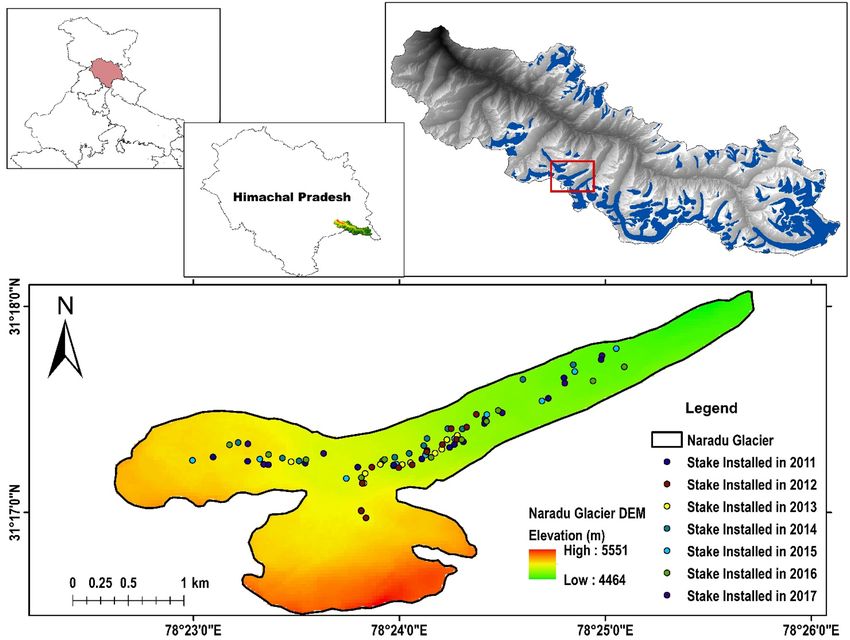
www.nature.com/scientificreports/
Figure 1. Location map of Naradu Glacier showing the network of stakes during the study periods. The map
has been prepared using geographical information system (ArcGIS 10.1; version 10.1 and authorization number:
EFL691568009-1010). (courtesy- India map shapefile at http://www.diva-gis.org/gdata; Digital Elevation Model
(DEM) download from NASA Earth Data at https://search.earthdata.nasa.gov/search/; Naradu glacier shapefile
digitized manually on Landsat 8 image acquired from USGS https://earthexplorer.usgs.gov/ dated 19 September
2019).
The Himalayan region comprises the largest glacier mass outside the polar areas, and this region is often
referred to as the ‘water tower of Asia’. The role of Himalayan originated rivers in providing fresh water to the
downstream population is very important, especially in the dry s eason34,35. Unfortunately, few mass balance
studies have been d one36–38 over different parts of the Himalayas. This shortcoming has been reported in the
Himalayan region and the entire world39. The main objective of this study is to estimate the mass balance of
Naradu Glacier, Western Himalaya, using the trendy glaciological method. The Glaciological mass balance of
Naradu Glacier has been calculated for seven continuous years to understand its considerable contribution to
the Baspa River and glacier sensitivity with changing climate.
Study area. Naradu Glacier is among 89 glaciers of Baspa basin, western Himalaya40 and contributes its
water to Baspa River. Baspa River joins Satluj River on its left bank near Karchham at an elevation of about
1770 m above sea level (m a.s.l.). Naradu Garang is a 3rd order stream of Sutluj and joins Baspa River on its left
bank opposite Chitkul village at an elevation of about 3450 m a.s.l. The glacier ranges between 78° 25′ 06.17″ to
78° 25′ 34.07″ E and 31° 17′ 27.1″ to 31° 18′ 18.9″ N and covers an area of 3.8 km240. It is a southwest-northeast
facing glacier and falls in the SOI toposheet No. 53I/07. Naradu Glacier is highly debris (thin to thick cover) cov-
ered, and debris extends to 37.92% of the total glacier area. The location map of Naradu Glacier with a network
of installed stakes during the study period is shown in Fig. 1 (prepared using geographical information system
(ArcGIS 10.1; version 10.1 and authorization number: EFL691568009-1010).
Climate dynamics of the valley. The Himalayan region’s hydrological cycle mainly depends on two cir-
culation systems, Indian Summer Monsoon (ISM) and Western Disturbance (WD)41–47. Glaciers of western
Himalaya have accumulated through WD mainly in January and February, while the eastern and central Hima-
layas’ glaciers are accumulated mainly through the summer monsoon48. Western disturbance is the non-mon-
Scientific Reports | (2021) 11:12710 | https://doi.org/10.1038/s41598-021-91348-3 2
Vol:.(1234567890)www.nature.com/scientificreports/
soonal precipitation driven by westerly wind directions, which brings sudden winter snow. The moisture of the
western disturbance originates over the Mediterranean S ea49. In the winter months, western disturbances reach
to lowest latitudes. In their way, they cross the north and central parts of India in a phased manner from west to
east, disturbing usual features of the circulation pattern50. This causes snowfall in higher elevations of NW India
and winter rainfall in plains of northern and central India. Baspa Basin falls in the western Himalayan Range and
hence receives its precipitation during winter months due to westerly disturbances. The study region receives
nearly 70% of annual precipitation as snowfall in winter and spring, and only 30% as rainfall near the glacier
termini and as dry snow in higher-up r egions37. The temperature analysis shows that the glacier’s monthly tem-
perature ranges from − 12.20 to 6.76 °C (Fig. S1a) between 2011–12 to 2017–18. The temperature trend analysis
during 1979–80 to 2012–13 showed an increase of 0.9 °C in mean air temperature, whereas precipitation shows
a decrease of 14.38 cm40.
Data description and glaciological mass balance methodology. The most precise method for
mass balance measurement is the glaciological method that utilizes the observations of differential exposure of
installed stakes in the ablation zone to estimate the melting and digging pits to measure the accumulation. For
our measurements, field visits were made during the last week of September to the first week of October during
the study period. About 4 to 6 bamboo stakes (each 1.5 m long) were installed using a portable steam drill51 at
different altitudes of the glacier in the ablation zone to measure the mass loss. The stakes’ differential exposure
every year gave the annual vertical thinning of the glacier mass at that location. The multiplied annual exposure
with the density of ice gives the specific mass balance at that glacier location. Density for ice is assumed constant
at 900 kg m−3.
The variation between the beginning and the end of a hydrologic year represents the mass balance change for
that year52–55. For the ablation measurement of Naradu Glacier, a network of stakes has been installed at different
altitudinal zones (covering a range of 50 to 100 m). The average ablation in each zone is computed by multiplying
the altitude band’s area with the melting observed at the representative stakes.
For net yearly ablation measurement, the length of stakes above the glacier surface has been measured at two
successive dates (t1 and t 2). The depth of snow (D) over the ice surface was also measured. The difference between
stake lengths buried in ice (L) and snow depths at t 1 and t2 dates gives the specific ablation (ΔS) at that point.
The exposure of stakes and snow depths were measured at each stake. The net ablation at a particular point is
calculated by using the formula given below:
�S = Di [L(t2 )−L(t1 )] + Ds [D(t2 )−D(t1 )] (1)
where S = Specific ablation (m w.e.), t1 = Year of initial measurement (cm), t2 = Year of subsequent measurement
(cm), L = Length of stakes buried in ice (cm), D = Depth of snow (cm), Di = Density of ice (g/cm3), Ds = Density
of snow (g/cm3).
Stakes above the glacier surface were measured every year from September 2012 to September 2018, with
ice/snow density and the emergence difference giving the annual ablation at that point.
The ablation and accumulation values have been integrated over the glacier to calculate the mass balance.
The overall mass balance, Bi is calculated according to:
Bi = S bi (si ) (2)
where bi is the mass balance (m w.e.) of the altitudinal range i of area si (m2) and S is the total glacier area
(km2). For each altitudinal range, bi is obtained from the corresponding stake readings or net accumulation
measurements.
Meteorological data and MLRA
To better understand the causes of glacier surface mass balance (SMB) variability, multiple linear regression
analysis (MLRA) is performed with temperature and precipitation series. For the analysis, monthly temperature
and precipitation data have been downloaded from NASA GIOVANNI’s website (Fig. S1a). GIOVANNI is the
acronym of Geospatial Interactive Online Visualization And aNalysis Infrastructure (Goddard Earth Sciences
Data Information Services Center). It is an online (web) environment for the display and analysis of geophysical
parameters. Data for both the parameters have been downloaded by selecting coordinates 31° 06′–31° 30′ N and
78° 12′–78° 37′ E with a grid size of 0.5° × 0.625° in the selected region. The GIOVANNI data has been carefully
analyzed for homogeneity. ANOVA test has been used to check the inhomogeneity in temperature data. In
contrast, due to the non-availability of real annual precipitation data, we cannot apply the same to precipitation
data. ANOVA test has been used by considering the field observations (through AWS) of yearly temperature data
for years 2012/13–2013/14 and 2015/16 to 2017/18. The test does not show any inhomogeneity as the calculated
value is less than the table value of ‘F’ at the 5% level. Further, it has been assumed that GIOVANNI data for pre-
cipitation is homogeneous. The data shows a lower winter temperature (Fig. S1b). This may be the consequence
of stronger winter inversion in the valley. An attempt has also been made to model the elevation against SMB.
For the same, a best fit linear Eq. (3) has been estimated considering all stakes.
SMB = 0.39 (±0.073) ∗ Elevation − 2167 (±355) (3)
where SMB is the annual specific mass balance (m w.e.), elevation represents the stake elevation (m a.s.l.) and
the uncertainties correspond to the 95% confidence level. Based on this simple linear fit approach, the average
ELA for the period of 2011/12–2017/18 is obtained at 4914 m a.s.l., which is under-estimated compared to actual
observations.
Scientific Reports | (2021) 11:12710 | https://doi.org/10.1038/s41598-021-91348-3 3
Vol.:(0123456789)www.nature.com/scientificreports/
1
0
Ablaon/Accumulaon (m w.e.)
-1
-2
-3
-4
-5
2011-12 2012-13 2013-14 2014-15 2015-16 2016-17 2017-18
-6
4500 4600 4700 4800 4900 5000 5100 5200 5300 5400
Elevaon ( m asl)
Figure 2. Specific accumulation/ablation with elevation during the ablation years 2011–12 to 2017–18. The
vertical error bars indicate the standard deviation (± 1σ) of the accumulation/ablation.
Year Net balance (105 m3) ELA (m a.s.l.) Sp. Bal. (m w.e.) Uncertainty (%)
2011/12 − 3.5 5209 − 1.09 2.6%
2012/13 − 3.7 5225 − 1.15 2.3%
2013/14 − 2.7 5196 − 0.86 1.3%
2014/15 − 2.5 5152 − 0.79 3.4%
2015/16 − 2.4 5135 − 0.77 1.6%
2016/17 − 2.0 5086 − 0.63 2.4%
2017/18 − 2.2 5127 − 0.69 2.1%
Average − 2.71 5161 − 0.85 2.24%
Table 1. Mass balance results for the period 2011–12 to 2017–18.
The stake’s elevation changes with time due to the melting of ice and glacial downward flow56–58. During seven
years, the total elevation change is around 253 m for stake 1, 210 m for stake 2, and 183 m for stake 3 (kindly
refer Statistical Analysis under Results and Discussion for Stake 1, 2 and 3 description). To analyze the effect of
elevation change on surface mass balance, all stakes (i.e., 1, 2 and 3) are adjusted back to their initial elevation
(i.e., 2011–12) by using Eq. (3). The observed and modeled surface mass balance (modeled surface mass balance
is the surface mass balance obtained by putting various elevations in Eq. (3)) analysis shows a moderate correla-
tion (R2 = 0.53). The modeled annual surface mass balance shows an average ablation of − 2.48 m w.e. a −1, which
does not significantly differ from the actual observed average ablation − 2.34 m w.e. a −1.
Results and discussion
Accumulation and Ablation analysis. The mass balance study on Naradu Glacier has started by Koul
and Ganjoo previously under the DST-funded project during 2000/01–2002/0337. The second series of mass bal-
ance has been performed under the DST sponsored project No. SR/ DGH/HP-1/2009 dated 09.09.2010 for the
year 2011/12–2013/14 followed by an extension of the activities for another four years (2014/15–2016/17) under
project no. SB/DGH-92/2014 dated 19/02/2015. Also, one more year (2017/18) fieldwork has been performed
to the Naradu Glacier to collect the data. The present study uses the most accurate glaciological data, and trendy
methods to calculate the mass b alance59 of Naradu Glacier for seven (2011–12 to 2017–18) years. In the entire
study period, 84 annual surface mass balance measurements at different glacier locations have been performed.
The specific ablation/accumulation with varying elevation in different years is shown in Fig. 2. All measurements
show a negative mass balance. The variation in equilibrium line altitude (ELA) in various years and net mass
balance is shown in Table 1.
The ablation estimation for the year 2011–12 is based on 13 stakes measurements, distributed between the
elevation range of 4590 to 5136 m a.s.l. on the glacier’s central line. Ablation at a specific location was measured
by observing the differential exposure of stakes yearly, preferable in the last week of September or 1st week of
October, depending on the weather condition. Four pits between the elevation range of 5152 to 5289 m a.s.l.
have been dug in the accumulation zone to obtain the annual specific accumulation. The subsequent years’ mass
Scientific Reports | (2021) 11:12710 | https://doi.org/10.1038/s41598-021-91348-3 4
Vol:.(1234567890)www.nature.com/scientificreports/
balance estimation is based on installing new stakes at new places and installing stakes to the earlier locations
to have continuity in the data series. The observations are made to all stakes (new and old), where the old stake’s
data provided the annual ablation of last year (2012–13). The new stake’s observation becomes the reference
data for next year’s ablation measurements. The accumulation estimation for 2012–13 is based on four snow
pits at the elevation range of 5132–5249 m a.s.l. Likewise, mass balance measurements for the years 2013–14,
2014–15, 2015–16, 2016–17, and 2017–18 have been made. During seven-year analysis, variation between low-
est and highest melting is − 0.1 m w.e. to − 5.1 m w.e. The highest melting zone for four years (i.e., 2011–15)
is at the elevation range of 4700–4800 m a.s.l. The topographic characteristics that play an important role in
glacier melting are glacier hypsometry, slope and a spect60. Given this, we attempted to study all the possible
topographic factors for Naradu Glacier, affecting the melting. We found that the south and southeast aspects,
debris cover area, and the slopes between 7 to 24 degrees are the significant factors that would have made this
zone the highest melting zone for four discussed years. The detailed map showing the aspect, debris, and slope
of Naradu Glacier has been demonstrated through Fig. 3a–c (prepared using geographical information system
(ArcGIS 10.1; version 10.1 and authorization number: EFL691568009-1010). During seven-year analysis, the year
2012–13 showed the highest ablation of − 1.15 m w.e. supported by the detailed analysis of temperature indices
showing comparatively high temperature during the same period. Along with temperature, net radiation, latent
heat flux, and other topographical characteristics also played a significant role.
Uncertainties of mass balance measurements. Worldwide, most of the mass balance calculations
are done only for a few years, and large numbers of results are reported without uncertainty e stimation20. A
longer series of mass balance (more than 40 years) has been reported only for 33 glaciers61, and quality matters
significantly in this kind of analysis. Various previous studies discussing errors in mass balance calculated by the
glaciological method are in the record. Many authors estimated errors between ± 0.2 and ± 0.4 m w.e.62–65. Meier
and others66 indicated errors between ± 0.1 and ± 0.34 m w.e. for mass balances determined by the glaciological
method. Lliboutry67, calculated an error of ± 0.19 m w.e. for ablation measured with stakes, whereas ± 0.3 m w.e.
of error was reported by Vallon and Leiva68. Gerbaux and others69 calculated the winter and summer balance
and found an error of ± 0.10 m w.e. for ablation measured in ice and between − 0.25 and + 0.4 m w.e. for ablation
measured in firn. Error estimation in mass balance studies using the glaciological method is a very important
issue. In this study, we have taken the utmost care in the measurements to reduce the possible errors. The error
due to the movement of ice is negligible because of the low velocity of glacial ice. The errors in joining stakes and
making a uniform surface at the bottom of the stakes have been carefully monitored and recorded.
Further to minimize the error in the average spatial result, many stake networks have been installed. In most
mass balance studies, glacier area has been taken to be invariant, whereas it changes with time in actual practice
and ultimately contributes to the overall error in the mass balance r esult36,70. To avoid this kind of errors, we have
used the most recent area images to calculate the surface mass balance of every year. Further, the uncertainty
related to the stake height determination, depth of snow in the ablation zone, and snow/ice density have been
considered to calculate overall uncertainty in calculating the surface mass balance of Naradu Glacier. Uncertainty
in the surface mass balance calculation of Naradu Glacier has been estimated using the equation suggested by
Gantayat et al. (2014)71 and mentioned in Table 1.
Statistical analysis. The study also aims to describe the observed surface mass balance (through MLRA)
using temperature and precipitation as predictors. The additional predictors can be added, but it increases the
fraction of surface mass balance variation, consequently reduces the degree of freedom. The p-value of the F-test
should be as low as possible to justify the addition of predictors. The analysis is only based on continuous peri-
ods.
The multiple linear regression analyses has been conducted by taking 21 surface mass balance measurements.
These 21 surface mass balances are based on three stake observations maintained by reinstalling to the following
year’s location, in case it appeared that it would not survive till next year. The ablation zone of Naradu Glacier
is a highly debris-covered area (refer to Fig. 3b) and may have a significant impact on the melting of ice/snow
depending on its t hickness72. MLRA does not include the surface mass balance measurements from the stakes
that could not survive for the whole study period. The involvement of these kinds of measurements will surely
raise the biases due to the gap in their data record56.
The specific mass balance measurements of three stakes are shown through Fig. S2 a and b. The annual abla-
tion is more than 6 m w.e. for all the balance years except 2014–15. Modeled surface mass balance values show
a significant increasing trend over seven years as the p-value of F-test is much lower than α = 0.01. The standard
deviation in surface mass balance per stake per year varied between 0.002–0.17 m w.e. a−1 and does not show
correlation with elevation (as R 2 = 0.07) (Fig. S3).
For further analysis, the modeled surface mass balance measurements for each stake are converted to per-
turbations by taking seven years stakes’ mean. The surface mass balance perturbation is shown in Fig. S4. We
found a perfect correlation between surface mass balance perturbation and elevation for all three stakes during
analysis. Further, no link has been found between meteorological parameters (i.e., temperature and precipitation)
and annual surface mass balance elevation gradient. The “no linkage” is a prerequisite condition for our analysis
and is in line with many other related studies eg.,73–76.
To understand the relation between meteorological parameters and surface mass balance perturbation, the
MLRA approach has been used by considering Eq. (4) 57,77. This correlation analysis requires the abandonment of
the effect of measurement of different meteorological parameters in other units (here, the temperature in degree C
and precipitation in mm w.e.). Hence, these parameters have been standardized by converting the data to z-score.
Scientific Reports | (2021) 11:12710 | https://doi.org/10.1038/s41598-021-91348-3 5
Vol.:(0123456789)www.nature.com/scientificreports/
Figure 3. Naradu Glacier map showing (a) aspect, (b) debris-covered area, and (c) slope of different elevation
zone. The map has been prepared using geographical information system (ArcGIS 10.1; version 10.1 and
authorization number: EFL691568009-1010). (courtesy- Digital Elevation Model (DEM) download from NASA
Earth Data at https://search.earthdata.nasa.gov/search/; Naradu glacier shapefile digitized manually on Landsat
8 image acquired from USGS https://earthexplorer.usgs.gov/ dated 19 September 2019).
Scientific Reports | (2021) 11:12710 | https://doi.org/10.1038/s41598-021-91348-3 6
Vol:.(1234567890)www.nature.com/scientificreports/
y = a1 x1 + a2 x2 + · · · an xn + b (4)
where y = dependent/response variable and indicates surface mass balance perturbation in the present study. ‘a’
and ‘b’ are the regression coefficients, and x 1, x2,…xn are the independent/predictor variables. Here, x1 andx2 is
represented by the z-score of the meteorological parameters, i.e., temperature and precipitation. The monthly
temperature and precipitation data show a weak correlation (R2 = 0.3), and this non-dependency is a common
approach for MLRA performed on surface mass balance series e.g.,56,78,79. We have converted the meteorological
data to a z-score. The regression coefficients ‘a1, a2…an.’ show the climatic variability of meteorological parameters.
Further, it has been assumed that the regression coefficients of both the parameters are uncorrelated and indicate
the importance of both for surface mass balance. The intercept of the regression analysis (i.e., ‘b’) is equal to zero
as it shows a value of y when all of the independent variables are equal to zero. The error degrees of freedom is
the difference product of the total number of years (i.e., 7 in this analysis) and the number of independent vari-
ables used in the analysis (here temperature and precipitation). The outcome of MLRA is expressed in terms of
R2 and p-value of the F-test. The factor R 2 shows the variability of the response variable. The F-test performs a
significant linear regression relationship between the response variable and the predictor variables. The p-value
of the F-test is the probability of obtaining a linear correlation if the null hypothesis is true. The lower p-value
at a higher significance level results in the rejection of the null hypothesis. We opted for a null hypothesis for
analysis that there is no linear correlation between the response variable and the predictor variable.
Firstly, the annual average temperature ( Tann) and total annual precipitation ( Pann) have been used to explain
the observed surface mass balance variation (MLRA with 5 error degrees of freedom). An MLRA shows that 71%
of the variance of observed surface mass balance can be explained by these two predictors. The lower p-value
of the F-test (0.07) describing the decisive significance of the model. The negative sign of T ann shows a negative
correlation between temperature and surface mass balance, and the positive sign of P ann shows a positive cor-
relation between precipitation and surface mass balance (refer to Fig. S5a and Table S1).
Secondly, the year is sub-divided into two categories, i.e., winter half-year (WHY) and summer half-year
(SHY). The first category, i.e., WHY consists of fall (OND: October, November, December) and winter (JFM:
January, February, March). The second category consists of spring (AMJ: April, May, June) and summer (JAS:
July, August, September). The chosen monthly combination does not agree with meteorological seasons. They
are selected according to the glaciological season so that the fall season (OND) should start just after field
measurement.
The MLRA shows the importance of SHY temperature. This variable alone explains the 64% variance of
observed surface mass balance (R2 = 64%; p-values F-test = 0.02). In the absence of this variable, no surface
mass balance variance can be explained in MLRA with two predictor variables (For example, R2 = 58%; p-values
F-test = 0.17) (Table S1). The summer temperature and winter precipitation account for 80% of the observed
surface mass balance variance (with p-value of F-test 0.03), hence the null hypothesis, no linear correlation has
been rejected. The larger absolute regression coefficient T SHY (− 73.5) compared with P WHY (+ 11.06) indicates a
relatively higher importance of the SHY temperature (Fig. S5b).
Thirdly, the predictors split into seasonal components, i.e., spring (AMJ), summer (JAS), autumn (OND),
and winter (JFM). This allows us to analyze 36 possible combinations for MLRAs using temperature and pre-
cipitation as a predictor variable. In the seasonal analysis, we found that with two predictor variables, most of
the surface mass balance variability is described by summer temperature and winter precipitation (R2 = 82%;
p-values F-test = 0.032) (refer to Table S1).
Depth analysis of all monthly combinations is also done, and the results show that the June temperature and
September precipitation best describe the surface mass balance variance. This MLRA is statistically significant
as it has much lower p-values F-test = 0.0031 and R 2 = 94%. The individual monthly equation (refer to Fig. S5c
and Table S1) indicates the dominance of temperature (regression coefficient of − 50.51) compared with the
September precipitation (regression coefficient of − 36.45).
Temperature dominance. The analysis shows that the observed surface mass balance and temperature are
strongly correlated. The same findings have been reported by Koul and Ganjoo37, in which they have assessed
the impact of inter and intra annual meteorological parameters variation on Naradu Glacier mass balance. Dur-
ing the analysis, the authors have estimated that the melting of Naradu Glacier is positively proportional to the
temperature, which is a function of solar radiation reaching on the glacier. Azam and others80 found that the
turbulent heat flux has a significant impact on the surface mass balance of Chhota Shigri Glacier and is closely
correlated with the temperature. The lack of such studies for nearby glaciers, which analyze the surface mass
balance variability and its causes related to the meteorological parameters, restrict us to present more evidence
in favor of the findings. The energy balance study of Naradu Glacier under the above-mentioned financial assis-
tance has been done for five non-continuous years (2012–14 and 2015–18). We found that radiation mechanisms
and sensible heat flux significantly drive the glacier’s specific energy balance in the analysis. This study finds that
temperature explains a significant fraction of the observed surface mass balance because it is the representative
index for solar radiation and sensible heat flux48,81.
The Naradu Glacier starts losing its mass from April and continues till September, and sometimes it extends
till mid-October. In these months, along with the high temperature, the snow cover reduction also plays a
vital role in glacier melting due to a decrease in albedo. The MLR analysis shows that the April to September
months’ temperature and precipitation conditions significantly affect surface mass balance variability. Among
all the monthly combinations, the variability is best described by June temperature and September precipita-
tion. The precipitation during these months occurs as rain which further enhances the melting along with the
high temperature.
Scientific Reports | (2021) 11:12710 | https://doi.org/10.1038/s41598-021-91348-3 7
Vol.:(0123456789)www.nature.com/scientificreports/
Naradu Glacier’s mass balance comparison with other glaciers of Indian Himalaya. The mass
balance study on Naradu Glacier has been performed by using the most accurate glaciological method. Very
few glaciological mass balance studies for a longer period have been reported in the Himalayan r egion19,21,82.
The available field-based glacier mass balance data from Indian Himalayan regions are presented in Fig. S6. In
Indian Himalaya, the Geological Survey of India (GSI) has started the detailed mass balance study using the
glaciological method in 1974. The study was undertaken on Gara Glacier, Himachal Pradesh, to understand
the glacial melt and its impact on local and regional hydrological systems. The Gara Glacier had been studied
during 1974–75 to 1981–8283,84. The study showed a positive mass balance for the years 1974–75, 1975–76, and
1981–82 and the rest of the five years showed a negative mass balance. These positive mass balance results are
dissimilar with most of the analyses done in the basin. The publication83 did not give any scientific reason behind
this behavior of the glacier. Likewise, the Nehnar, Kashmir Himalaya glacier has been studied continuously for
8 years between 1975–76 to 1983–84. The study is one among many glaciers that has the longest glaciological
mass balance record in the region. The scientific team involved in the study reported the negative mass balance
for the entire study period, which ranges from − 0.4 to − 0.7 m w.e.85. The Shaune Garang Glacier has the longest
study series (10 years or more) in the Baspa basin, showed a positive mass balance only for two years, and the rest
eight years showed significant mass loss86,87. Later on, the reconstruction of mass balance on the same glacier has
been done by Kumar and o thers88 for 2001–02 to 2007–08. In this reconstruction analysis, the authors found a
negative mass balance for five years, whereas the glacier gained the mass in 2001–02 and 2004–05. On average,
the results of Shaune Garang Glacier show more mass loss compared to Naradu Glacier. This high melting at
Shaune Garang Glacier may be linked with the high temperature and lower precipitation c onditions89. Another
glacier with the longest study series outside the Baspa basin is the Chhota Shigri Glacier90 which is well-studied
in many aspects. The glacier has been studied for mass balance, energy balance, and the reconstruction of the
mass balance for over 43 years (1969–2012). The mass balance reconstruction for over 43 years was done to get
the larger perspective of a glacier-climate relationship. The glacier reconstruction study shows that the abla-
tion was more for most of the study years than the positive value. Likewise, the glacier’s mass balance using the
glaciological method shows a negative mass balance for most of the study period. The marginal positive values
were reported for the years 2004–05; 2008–09, and 2009–1080. Smaller duration mass balance studies have been
reported from other glaciers like Rulung, Kolahoi II, Shishram, which showed the negative mass b alance19.
Nine long-year analyses of the mass balance of Gor Garang Glacier, Baspa basin showed a negative mass bal-
ance for seven years and a minimal positive mass balance for two y ears19,84. The Dunagiri and Chorabari Glaciers
of Uttarakhand Himalaya have been studied for six and more years and have been reported with negative mass
balance91–93. The mass balance of Dokriyani Glacier for six y ears92 showed a negative trend. The reported reason
was less winter precipitation, which causes longer period exposure of the glacier surface ice for melting. Less
precipitation during the winter season leads to less input to the accumulation zone of the glacier. Hamta and
Naradu Glacier of the western Himalayan region has been studied for 11 (2000–2009 and 2010–2012) and 3
(2000–2003) years, respectively. Both the glaciers showed a negative mass b alance37,94,95.
Other MLRA studies. Similar studies are limited in western Himalaya, which is extended throughout the
Himalayan region96. The studies analyzing the effect of temperature and precipitation on surface mass balance
variation found that surface mass balance is more sensitive to temperature rather than p recipitation56,97. Still,
the scenario may change depending on the spatial locations98, resulting in the change in the magnitude of vari-
ous meteorological parameters. The same findings have been reported by Kayastha and others99. This study was
done on Glacier AXOIO in the Nepalese Himalaya by taking three predictors: air temperature, precipitation,
and relative humidity. The study results showed that mass balance is more sensitive to air temperature as apart
from melting, it also controls the phase of precipitation (snow or rain). In 2017, Gaddam and others did the same
study by taking four glaciers from the western Himalaya (three glaciers of the Baspa basin and one glacier from
the Gara Khad basin)89. It has been reported that during the ablation season, the temperature perturbations were
higher, whereas precipitation perturbations were higher during the accumulation season. The findings are same
in our analysis, but there may be a difference in the magnitude of melting as the above study includes October
month in the ablation period (in the present study, months from April to September defines the ablation season).
Wang and others did a recent study at 45 glaciers of the Tianshan Mountains and Central Himalayan Mountains.
They reported a linear increase in mass balance with the rise in perturbation of p recipitation100. Our results are
in agreement as the quantity and form of precipitation depend on temperature.
In 2015, Engelhardt and o thers101 analyzed four glaciers of Norway using the sensitivity formula given b y102.
In this analysis, Engelhardt found that at a higher temperature, surface mass balance sensitivity to temperature
increases, whereas surface mass balance sensitivity to precipitation decreases. This shows that the sensitivity of
surface mass balance also depends on the magnitude of temperature and precipitation; for example, higher tem-
perature causes the reduction in the accumulation period and reduces the amount of precipitation as snow. Our
continuous monthly period analysis shows a higher correlation compared with other s tudies56. This may happen
because their analysis was based on many variables, i.e., May–June–July temperature and winter precipitation
(here, we took June temperature and September precipitation). Apart from variation in the variables, the results
also depend on the data quality (here, we took meteorological data from NASA GIOVANNI and field-based
surface mass balance) and preprocessing before use. The validation of the satellite data with field data is a must
for checking the homogeneity.
Scientific Reports | (2021) 11:12710 | https://doi.org/10.1038/s41598-021-91348-3 8
Vol:.(1234567890)www.nature.com/scientificreports/
Conclusions
This study uses the most accurate glaciological method to estimate the mass balance of Naradu Glacier of the
Baspa basin for seven continuous years. The annual surface mass balance of Naradu Glacier for the period of
2011–12 to 2017–18 showed a negative trend with the maximum deficit of − 1.15 m w.e. in 2012–13. The direct
melting proportionality with the temperature makes this glacier witness to the higher sensitivity to temperature
change. In Indian Himalaya, mass balance studies started back in 1974 and covered different glaciers for differ-
ent periods. The studies reported so far confirm that almost all the glaciers under investigation have gone to a
negative mass balance state except for a few with the marginal positive values (e.g., Gara Glacier, Shaune Garang
Glacier, and Chhota Shigri Glacier). This indicates that the Baspa basin and the entire Indian Himalayas are expe-
riencing a negative mass balance. Although in recent decades interest of the research community has increased to
explore the glaciers of Indian Himalayan Region (IHR) yet the present study suggests that more attention should
be given to glaciological mass balance studies as they are very few in numbers and hence the understanding of
glaciers’ spatial and temporal variability is weak compared to the other world’s mountain glaciers. This study also
describes the surface mass balance variation through MLRA by taking temperature and precipitation variables.
The authors did not add other meteorological parameters (such as solar radiation, relative humidity, etc.) in the
analysis as temperature and precipitation alone describe 71% of the observed surface mass balance variance. The
research shows surface mass balance variation can be better characterized by summer temperature rather than
precipitation. The summer temperature is an important variable explaining 64% variance of observed surface
mass balance with p-values F-test = 0.02, which is quite satisfactory. The seasonal analysis with two predictor
variables shows that most of the surface mass balance variability is described by summer temperature and winter
precipitation (R2 = 82%; p-values F-test = 0.032). The monthly analysis indicates that high temperatures and low
precipitation in June cause much of the snow to be melted out, exposing ice surfaces, resulting in lower albedo.
Further, the type of precipitation (rain/snow) also influences the surface mass balance over the Naradu Glacier.
Received: 19 November 2020; Accepted: 17 May 2021
References
1. IPCC, (2018). Summary for Policymakers. In: Global Warming of 1.5 °C. An IPCC Special Report on the impacts of global warm-
ing of 1.5 °C above pre-industrial levels and related global greenhouse gas emission pathways, in the context of strengthening
the global response to the threat of climate change, sustainable development, and efforts to eradicate poverty [Masson-Delmotte,
V., P. Zhai, H.-O. Pörtner, D. Roberts, J. Skea, P.R. Shukla, A. Pirani, W. Moufouma-Okia, C. Péan, R. Pidcock, S. Connors, J.B.R.
Matthews, Y. Chen, X. Zhou, M.I. Gomis, E. Lonnoy, T. Maycock, M. Tignor, and T. Waterfield (eds.)]. World Meteorological
Organization, Geneva, Switzerland, 32 pp.
2. Jacob, T., Wahr, J., Pfeffer, W. T. & Swenson, S. Recent contributions of glaciers and ice caps to sea level rise. Nature 482, 514–518.
https://doi.org/10.1038/nature10847 (2012).
3. Chen, J. L., Wilson, C. R. & Tapley, B. D. Contributions of ice sheet and mountain glacier melt to recent sea level rise. Nat. Geosci.
6, 549–552. https://doi.org/10.1038/ngeo1829 (2013).
4. IPCC, (2013). “Summary for Policymakers,” in Climate Change 2013: The Physical Science Basis. Contribution of Working Group
I to the Fifth Assessment Report of the Intergovernmental Panel on Climate Change, eds T. F. Stocker, D. Qin, G. K. Plattner, M.
Tignor, S. K. Allen, J. Boschung, A. Nauels, Y. Xia, V. Bex, and P. M. Midgley (Cambridge; New York, NY: Cambridge University
Press).
5. Solomina, O. N. et al. Holocene glacier fluctuations. Quat. Sci. Rev. 111, 9–34 (2015).
6. Solomina, O. N. et al. Glacier fluctuations during the past 2000 years. Quat. Sci. Rev. 149, 61–90 (2016).
7. WGMS (2017). Global Glacier Change Bulletin No., 22014–2015), eds M. Zemp, S. U. Nussbaumer, I. Gärtner Roer, J. Huber,
H.Machguth, F. Paul, and M. Hoelzle (Zurich: ICSU(WDS)/IUGG(IACS)/UNEP/UNESCO/WMO, World Glacier Monitoring
Service).
8. Meier, M. F., & Tangborn, W. V. (1961). “Distinctive characteristics of glacier runoff,” in U.S. Geological Survey Professional
Paper 424-B, P14-B16.
9. Medwedeff, W. G. & Roe, G. H. Trends and variability in the global dataset of glacier mass balance. Clim. Dynam. 48, 3085.
https://doi.org/10.1007/s00382-016-3253-x (2017).
10. Meier, M. F. Contribution of small glaciers to global sea level. Science 226, 1418–1421. https://d oi.o
rg/1 0.1 126/s cienc e.2 26.4 681.
1418 (1984).
11. Oerlemans, J. & Fortuin, J. P. Sensitivity of glaciers and small ice caps to greenhouse warming. Science 258, 115–117. https://
doi.org/10.1126/science.258.5079.115 (1992).
12. Kuhn, M. (1993). “Possible future contributions to sea level change from small glaciers”–Chapter 8 in Climate and Sea Level
Change Observations, Projections and Implications, eds R.A. Warrick, E.M. Barrow, and T.M.L. Wigley (Cambridge: Cambridge
University Press), 134–143.
13. Dyurgerov, M. B. & Meier, M. F. Mass balance of mountain and subpolar glaciers: a new global assessment for 1961–1990. Arctic
Alpine Res. 29, 379–391. https://doi.org/10.2307/1551986 (1997).
14. Gregory, J. M. & Oerlemans, J. Simulated future sea-level rise due to glacier melt based on regionally and seasonally resolved
temperature changes. Nature 391, 474–476. https://doi.org/10.1038/35119 (1998).
15. Oerlemans, J. Estimating response times of Vadret da Morteratsch, Vadret da Palu, Briksdalsbreen and Nigardsbreen from their
length records. J. Glaciol. 53, 357–362. https://doi.org/10.3189/002214307783258387 (2007).
16. Paterson, W. S. B. The Physics of Glaciers 3rd edn. (Pergamon Press, 1994).
17. Oerlemans, J. Glaciers and Climate Change (AA Balkema, 2001).
18. Braithwaite, R. J. Glacier mass balance: the first 50 years of international monitoring. Prog. Phys. Geogr. 26, 76–95. https://doi.
org/10.1191/0309133302pp326ra (2002).
19. Dyurgerov, M. B., & Meier, M. F., (2005). Glaciers and the Changing Earth System: a 2004 snapshot. in Colorado, Institute of
Arctic and Alpine Research. University of Colorado, Occasional Paper, (Boulder, CO), 117.
20. Zemp, M., Hoelzle, M. & Haeberli, W. Six decades of glacier mass balance observations: a review of the worldwide monitoring
network. Ann. Glaciol. 50, 101–111. https://doi.org/10.3189/172756409787769591 (2009).
21. Cogley, J. G. Present and future states of Himalaya and Karakoram glaciers. Ann. Glaciol. 52, 68–73. https://doi.org/10.3189/
172756411799096277 (2011).
Scientific Reports | (2021) 11:12710 | https://doi.org/10.1038/s41598-021-91348-3 9
Vol.:(0123456789)www.nature.com/scientificreports/
22. Kaser, G., Cogley, J. G., Dyurgerov, M. B., Meier, M. F. & Ohmura, A. Mass balance of glaciers and ice caps: consensus estimates
for 1961–2004. Geopyhs. Res. Lett. 33, L19501. https://doi.org/10.1029/2006GL027511 (2006).
23. Hewitt, K. The Karakoram anomaly? Glacier expansion and the “elevation effect”, Karakoram Himalaya. Mt. Res. Dev. 25(4),
332–340. https://doi.org/10.1659/0276-4741(2005)025%5B0332:TKAGEA%5D2.0.CO;2 (2005).
24. Kääb, A., Berthier, E., Nuth, C., Gardelle, J. & Arnaud, Y. Contrasting patterns of early twenty-first-century glacier mass change
in the Himalayas. Nature 488, 495–498. https://doi.org/10.1038/nature11324 (2012).
25. Gardelle, J., Berthier, E. & Arnaud, Y. Slight mass gain of Karakoram glaciers in the early twenty-first century. Nat. Geosci. 5,
322–325. https://doi.org/10.1038/ngeo1450 (2012).
26. Gardelle, J., Berthier, E., Arnaud, Y. & Kääb, A. Region-wide glacier mass balances over the Pamir-Karakoram-Himalaya during
1999–2011. Cryosphere 7, 1263–1286. https://doi.org/10.5194/tc7-1263-2013 (2013).
27. Gardner, A. S. et al. A reconciled estimate of Glacier contributions to sea level rise: 2003 to 2009. Science 340, 852–857. https://
doi.org/10.1126/science.1234532 (2013).
28. Kumar, P. et al. Response of Karakoram-Himalayan glaciers to climate variability and climatic change: a regional climate model
assessment. Geophys. Res. Lett. https://doi.org/10.1002/2015GL063392 (2015).
29. Fountain, A. G. & Tangborn, W. V. The effect of glaciers on stream flow variations. Water Resour. Res. 21, 579–586. https://doi.
org/10.1029/WR021i004p00579 (1985).
30. Bakalov, V. D., Groman, D. S., Zalikhanov, M., & Ch., Panov, V. D. (1990). Upravlenierezhimomgornikhlednikov I stokomrek.
(Regime Control of MountainGlaciers and Glacier Rivers Flow-Off). Leningrad: Hydrometeoizdat.
31. Kaser, G., Grosshauser, M. & Marzeion, B. Contribution potential of glaciers to water availability in different climate regimes.
Proc. Natl Acad. Sci. U.S.A. 107, 20223–20227. https://doi.org/10.1073/pnas.1008162107 (2010).
32. Shrestha, A. B., Agrawal, N. K., Alfthan, B., Bajracharya, S. R., Maréchal, J., and van Oort, B., (eds.). 2015. The Himalayan Climate
and Water Atlas: Impact of Climate Change on Water Resources in Five of Asia’s Major River Basins. ICIMOD, GRID-Arendal
and CICERO.
33. WGMS, Glacier Mass Balance Bulletin No. 12 (2010–2011), Zemp, M., Nussbaumer, S.U., Naegeli, K., G€artner-Roer, I., Paul,
F., Hoelzle, M., Haeberli, W., 2013. ICSU (WDS)/IUGG(IACS)/UNEP/UNESCO/WMO. World Glacier Monitoring Service,
Zurich, Switzerland, pp. 58–60.
34. Siderius, C. et al. Snowmelt contributions to discharge of the Ganges. Sci. Total Environ. https://d oi.o rg/1 0.1 016/j.s citot env.2 013.
05.084 (2013).
35. Wahid, S., Shrestha, A., Murthy, M., Matin, M., Zhang, J., & Siddiqui, O. (2014). Regional Water Security in the Hindu Kush
Himalayan Region: Role of Geospatial Science and Tools. ISPRS - International Archives of the Photogrammetry, Remote Sens-
ing and Spatial Information Sciences. XL-8. 1331-1340. 10.5194/isprsarchives-XL-8-1331-2014.
36. Berthier, E. et al. Remote sensing estimates of glacier mass balances in the Himachal Pradesh (Western Himalaya, India). Remote
Sens. Environ. 108, 327–338. https://doi.org/10.1016/j.rse.2006.11.017 (2007).
37. Koul, M. N. & Ganjoo, R. K. Impact of inter- and intra-annual variation in weather parameters on mass balance and equilibrium
line altitude of Naradu Glacier (Himachal Pradesh), NW Himalaya, India. Clim. Change 99, 119–139. https://doi.org/10.1007/
s10584-009-9660-9 (2010).
38. Vincent, C. et al. Balanced conditions or slight mass gain of glaciers in the Lahaul and Spiti region (northern India, Himalaya)
during the nineties preceded recent mass loss. Cryosphere 7, 569–582. https://doi.org/10.5194/tc-7-569-2013 (2013).
39. Zhang, R. et al. A tree ring-based record of annual mass balance changes for the TS. Tuyuksuyskiy Glacier and its linkages to
climate change in the Tianshan Mountains. Quatern. Sci. Rev. 205, 10–21 (2019).
40. Singh, S., & Kumar, R. (2020). A statistical approach to estimate equilibrium line altitude (ELA) and its trend analysis on Naradu
Glacier, Himachal Himalaya. Materials Today: Proceedings. Accepted.
41. Pisharoty, P. & Desai, B. N. Western disturbances and Indian weather. Indian J. Meteorol. Geophys. 7, 333–338 (1956).
42. Rao, Y. P., Srinivasan, V., (1969). Forecasting manual, part II: discussion of typical synoptic weather situation: winter western
disturbances and their associated feature. FMU report no III-1.1, issued by India meteorological Department, India.
43. Singh, M. S. Westerly upper air troughs and development of western disturbances over India. Mausam 30, 405–414 (1979).
44. Kalsi, S. R. On some aspects of interaction between middle latitude westerlies and monsoon circulation. Mausam 38, 305–308
(1980).
45. Kalsi, S. R. & Haldar, S. R. Satellite observations of interaction between tropics and mid-latitude. Mausam 43, 59–64 (1992).
46. Dimri, A. P. & Mohanty, U. C. Simulation of mesoscale features associated with intense western disturbances over western
Himalayas. Meteorol. Appl. 16, 289–308 (2009).
47. Bookhagen, B. & Burbank, D. W. Toward a complete Himalayan hydrological budget: spatiotemporal distribution of snowmelt
and rainfall and their impact on river discharge. J. Geophys. Res. Earth Surf. 115(F3), 1–25. https://doi.org/10.1029/2009JF0014
26 (2010).
48. Ageta, Y. & Higuchi, K. Estimation of mass balance components of a summer-accumulation type glacier in the Nepal Himalaya.
Geogr. Ann. Ser. Phys. Geogr. 66, 249–255 (1984).
49. Hatwar, H. R., Yadav, B. P. & Rama Rao, Y. V. Prediction of western disturbances over Western Himalaya. Current Sci. 2005,
913–920 (2005).
50. Yadav, R. K., Kumar, K. R. & Rajeevan, M. Out of phase relationship between convection over northwest India and warm pool
region during winter seasons. Int. J. Climatol. 29, 1330–1338 (2009).
51. Heucke, E. A light portable steam-driven ice drill suitable for drilling holes in ice and firn. Geogr. Ann. Ser. B 81(4), 603–609.
https://doi.org/10.1111/j.0435-3676.1999.00088.x (1999).
52. Dyurgerov, M. B. (2002). Glacier Mass Balance and Regime: Data of Measurements and Analysis. Occasional Paper 55, Boulder,
CO: Institute of Arctic and Alpine Research, University of Colorado.
53. Kaser, G., Fountain, A. and Jansson. P. (2003). A manual for monitoring the mass balance of mountain glaciers. International
Hydrological Programme Technical Documents in Hydrology No. 59, Paris: UNESCO.
54. Hagen, J. O. & Reeh, N. In situ measurement techniques: land ice. In Mass Balance of the Cryosphere: Observation and modelling
of contemporary and future changes (eds Bamber, J. L. & Payne, A. J.) 11–42 (Cambridge University Press, 2003).
55. Hubbard, B. & Glasser, N. Field Techniques in Glaciology and Glacial Geomorphology (Wiley, 2005).
56. Zekollari, H. & Huybrechts, P. Statistical modelling of the surface mass-balance variability of the Morteratsch glacier, Switzerland:
strong control of early melting season meteorological conditions. J. Glaciol. 64(244), 275–288. https://doi.org/10.1017/jog.2018.
18 (2018).
57. Zekollari, H., Fürst, J. J. & Huybrechts, P. Modelling the evolution of Vadret da Morteratsch, Switzerland, since the little Ice Age
and into the future. J. Glaciol. 60(224), 1208–1220. https://doi.org/10.3189/2014JoG14J053 (2014).
58. Fischer, M., Huss, M. & Hoelzle, M. Surface elevation and mass changes of all Swiss glaciers 1980–2010. Cryosphere 9(2), 525–540.
https://doi.org/10.5194/tc-9-525-2015 (2015).
59. Østrem, G. & Brugman, M. (1991). Glacier mass balance measurements: A manual for field and ice work, Science Report.
National Hydrological Research Institute, Saskatoon/Norwegian water recourse and electricity board, Oslo.
60. Pandey, P., Nawaz Ali, S., Ramanathan, A. L., Champati Raya, P. K. & Venkataram, G. Regional representation of glaciers in
Chandra Basin region, western Himalaya. India. Geosci. Front. 8, 841–850. https://doi.org/10.1016/j.gsf.2016.06.006 (2017).
Scientific Reports | (2021) 11:12710 | https://doi.org/10.1038/s41598-021-91348-3 10
Vol:.(1234567890)www.nature.com/scientificreports/
61. Dyurgerov, M. B. & Meier, M. F. Analysis of winter and summer glacier mass balances. Geografiska Annaler Ser. A Phys. Geography
81A(4), 541–554 (1999).
62. Braithwaite, R. J. Assessment of mass balance variations within a sparse stake network, Qamanarsupsermia, West Greenland. J.
Glaciol. 32(110), 50–53 (1986).
63. Cogley, J. G. & Adams, W. P. Mass balance of glaciers other than ice sheets. J. Glaciol. 44(147), 315–325 (1998).
64. Braithwaite, R. J., Konzelmann, T., Marty, C. & Olesen, O. B. Errors in daily ablation measurement in northern Greenland,
1993–94, and their implication for glacier climate studies. J. Glaciol. 44(148), 583–588 (1998).
65. Cox, L. H. & March, R. S. Comparison of geodetic and glaciological mass balance techniques, Gulkana Glacier, Alaska, USA. J.
Glaciol. 50(170), 363–369 (2004).
66. Meier, M. F., Tangborn, W. V., Mayo, L. R., Post. A. (1971). Combined ice and water balances of Gulkana and Wolverine Glaciers.
Alaska, and South Cascade Glacier, Washington, 1965 and 1966 hydrological years”. Professional Paper 715-A, U.S. Geological
Survey, Fairbanks, Alaska.
67. Lliboutry, L. Multivariate statistical analysis of glacier annual balances. J. Glaciol. 13(69), 371–392 (1974).
68. Vallon, M. & Leiva, J. C. Bilan de masse et fluctuations récentes du glacier de Saint-Sorlin Alpesfrançaises. Zeitschriftfür
Gletscherkunde und Glazialgeologie 10(2), 143–167 (1981).
69. Gerbaux, M., Genthon, C., Etchevers, P., Vincent, C. & Dedieu, J. P. Surface mass balance of glaciers in the French Alps: distrib-
uted modelling and sensitivity to climate change. J. Glaciol. 51(175), 561–572 (2005).
70. Sourco, A. et al. Mass balance of Glacier Zongo, Boloivia, between 1956 and 2006, using glaciological, hydrological and geodetic
methods. Ann. Glaciol. 2009, 1–8 (2009).
71. Gantayat, P., Kulkarni, A. V. & Srinivasan, J. Estimation of ice thickness using surface velocities and slope: case study at Gangotri
Glacier, India. J. Glaciol. 60(220), 277–282 (2014).
72. Pratap, B., Dobhal, D., Mehta, M. & Bhambri, R. Influence of debris cover and altitude on glacier surface melting: A case study
on Dokriani Glacier, central Himalaya, India. Ann. Glaciol. 56, 9–16. https://doi.org/10.3189/2015AoG70A971 (2014).
73. Meier, M. F. & Tangborn, W. V. Net budget and flow of South Cascade Glacier, Washington. Glaciol 5(41), 547–566 (1965).
74. Kuhn, M. Mass budget imbalances as criterion for a climatic classification of glaciers. Geogr. Ann. Ser. A Phys. Geogr. 66(3),
229–238 (1984).
75. Rasmussen, L. A. Altitude variation of glacier mass balance in Scandinavia. Geophys. Res. Lett. 31, L13401. https://doi.org/10.
1029/2004GL020273 (2004).
76. Eckert, N., Baya, H., Thibert, E. & Vincent, C. Extracting the temporal signal from a winter and summer mass-balance series:
application to a six-decade record at Glacier de Sarennes, French Alps. J. Glaciol. 57(201), 134–150. https://doi.org/10.3189/
002214311795306673 (2011).
77. Legendre, P. & Legendre, L. Numerical ecology 3rd edn. (Elsevier, 2012).
78. Lefauconnier, B., Hagen, J. O., Ørbæk, J. B., Melvold, K. & Isaksson, E. Glacier balance trends in the Kongsfjorden area, western
Spitsbergen, Svalbard, in relation to the climate. Polar Res. 18(2), 307–313. https://doi.org/10.1111/j.1751-8369.1999.tb00308.x
(1999).
79. Trachsel, M. & Nesje, A. Modelling annual mass balances of eight Scandinavian glaciers using statistical models. Cryosphere
9(4), 1401–1414. https://doi.org/10.5194/tc-9-1401-2015 (2015).
80. Azam, M. F. et al. From balance to imbalance: a shift in the dynamic behaviour of Chhota Shigri Glacier (Western Himalaya,
India). J. Glaciol. 58, 315–324. https://doi.org/10.3189/2012JoG11J123 (2012).
81. Yanjun, C., Mingjun, Z., Zhongqin, Li., Yanqiang, W., Zhuotong, N., Huilin, L., Shengjie, W., & Bo, S. (2019). Energy balance
model of mass balance and its sensitivity to meteorological variability on Urumqi River Glacier No.1 in the Chinese Tien Shan.
Scientific Reports, volume 9, Article number: 13958.
82. Cogley, J. G. Geodetic and direct mass-balance measurements: comparison and joint analysis. Ann. Glaciol. 50, 96–100. https://
doi.org/10.3189/172756409787769744 (2009).
83. Raina, V. K., Kaul, M. K. & Singh, S. Mass-balance studies of Gara glacier. J. Glaciol. 18, 415–423. https://doi.org/10.1017/S0022
143000021092 (1977).
84. Raina, V. K. (2009). A State-of-Art Review of Glacial Studies, Glacial Retreat and Climate Change. Discussion Paper, MOEF,
New Delhi. Available online at: http://www.moef.nic.in/sites/default/files/MoEF%20Discussion%20Paper%20_him.pdf
85. Srivastava, D., Singh, R. K., Bajpai, I. P., & Roy, A. J. K. (1999). Mass balance of Neh Nar Glacier, District Anantang, J&K, in
Proceedings of the Symposium on Snow, Ice and Glaciers–a Himalayan perspective.
86. Singh, R. K., & Sangewar, C. V. (1989). Mass balance variation and its impact on glacier flow movement at Shaune Garang Glacier,
Kinnaur, Himachal Pradesh, in Proceedings National Meet on Himalayan Glaciology (New Delhi: Department of Science and
Technology), 149–152.
87. Mukherjee, B. P., & Sangewar, C. V. (1996). Correlation of accumulation area ratio and equilibrium-line altitude with the mass
balance of Gara, Gor Garang and Shaune Garang Glaciers of Himachal Pradesh, in Proceeding of the Symposium NW Himalaya
and Fore Deep GSI Special Publication, 303–305.
88. Kumar, R. et al. Development of a Glacio-hydrological model for discharge and mass balance reconstruction. J. Water Resour.
Manag. https://doi.org/10.1007/s11269-016-1364-0 (2016).
89. Gaddam, V. K., Kulkarni, A. V. & Gupta, A. K. Reconstruction of specific mass balance for glaciers in Western Himalaya using
seasonal sensitivity characteristic(s). J. Earth Syst. Sci. 126, 55. https://doi.org/10.1007/s12040-017-0839-6 (2017).
90. Wagnon, P. et al. Four years of mass balance on Chhota Shigri Glacier, Himachal Pradesh, India, a new benchmark glacier in
the western Himalaya. J. Glaciol. 53, 603–611. https://doi.org/10.3189/002214307784409306 (2007).
91. Geological Survey of India (GSI), (1992). Geological Survey of India (GSI): Glaciological studies on Dunagiri Glacier, district
Chamoli (Field Seasons 1983–84 to 1991–92), Final Report 1992 (Geological Survey of India), 5–9.
92. Dobhal, D. P., Gergan, J. T. & Thayyen, R. J. Mass balance studies of the Dokriani Glacier from 1992 to 2000, Garhwal Himalaya.
India. Bull. Glaciol. Res. 25, 9–17 (2008).
93. Dobhal, D. P., Mehta, M. & Srivastava, D. Influence of debris cover on terminus retreat and mass changes of Chorabari Glacier,
Garhwal region, central Himalaya, India. J. Glaciol. 59, 961–971. https://doi.org/10.3189/2013JoG12J180 (2013).
94. Mishra, R., Kumar, A. & Singh, D. Long term monitoring of mass balance of Hamtah Glacier, Lahaul and Spiti district, Himachal
Pradesh. Geol. Surv. India 147(Pt 8), 230–231 (2014).
95. Shukla, S. P., Mishra, R. & Chitranshi, A. Dynamics of Hamtah Glacier, Lahaul & Spiti district, Himachal Pradesh. Ind. Goephys.
Union 19, 414–421 (2015).
96. Kumar, P. et al. Snowfall variability dictates Glacier mass balance variability in Himalaya-Karakoram. Sci. Rep. 9, 18192. https://
doi.org/10.1038/s41598-019-54553-9 (2019).
97. Sakai, A. & Fujita, K. Contrasting glacier responses to recent climate change in high mountain Asia. Sci. Rep. 7, 13717. https://
doi.org/10.1038/s41598-017-14256-5 (2017).
98. Singh, S., Kumar, R. & Dimri, A. P. Mass balance status of Indian Himalayan Glaciers: a brief review front. Environ. Sci. https://
doi.org/10.3389/fenvs.2018.00030 (2018).
99. Kayastha, R. B., Ohata, T. & Ageta, Y. Application of a mass-balance model to a Himalayan Glacier. J. Glaciol. 45, 559–567 (1999).
100. Wang, R., Liu, S., Shangguan, D., Radic, V. & Zhang, Y. Spatial heterogeneity in Glacier mass-balance sensitivity across high
mountain Asia. Water 11, 776. https://doi.org/10.3390/w11040776 (2019).
Scientific Reports | (2021) 11:12710 | https://doi.org/10.1038/s41598-021-91348-3 11
Vol.:(0123456789)You can also read