Measuring earnings inequality in South Africa using household survey and administrative tax microdata - WIDER Working Paper 2021/82

WIDER Working Paper 2021/82

Measuring earnings inequality in South Africa
using household survey and administrative tax
microdata

Andrew Kerr*

May 2021

Abstract: Overall income inequality in South Africa is very high, and inequality generated in the
labour market is a key driver of inequality. In this paper, I use the Post-Apartheid Labour Market
Series, the General Household Surveys, and administrative tax microdata to describe earnings
inequality in South Africa. I estimate Gini coefficients, the variance of log earnings, and various
percentile ratios to document changes in earnings inequality. I show that earnings inequality
estimates from the Quarterly Labour Force Surveys are unreliable, most likely as a result of the
earnings imputations in the publicly available data from Statistics South Africa. I also use the tax
microdata to document the contributions of within- and between-firm differences to overall
earnings inequality.
Key words: inequality, earnings, administrative tax microdata, surveys, South Africa
JEL classification: D31, J31, O15
Note: figures and tables at the end
Acknowledgements: This paper has been supported by the UNU-WIDER SA-TIED
programme. The data is made available through cooperation between the South African Revenue
Service, the South African National Treasury, and UNU-WIDER. I thank Andrew Donaldson,
Amina Ebrahim, Aroop Chatterjee, Chris Axelson, Aalia Cassim, and participants at a 2021
SALDRU seminar for very helpful comments. I also thank Grace Bridgman, Singita Rikhotso,
Michael Kilumelume, Dane Brink, and Michelle Place from UNU-WIDER for all their help in
using the IRP5 administrative tax data remotely. The output from this paper has been checked so
that it does not compromise the anonymity of any firms or workers.

An earlier version of the paper was presented at the Centre for the Study of African Economies
Conference, University of Oxford, 2018, with Andrew Kerr and Aroop Chatterjee as authors. See
https://editorialexpress.com/cgi-bin/conference/download.cgi?db_name=CSAE2018&paper_
id=888.

* School of Economics and DataFirst, University of Cape Town, South Africa, andrew.kerr@uct.ac.za
This study has been prepared within the UNU-WIDER project Southern Africa—Towards Inclusive Economic Development
(SA-TIED).
Copyright © UNU-WIDER 2021
UNU-WIDER employs a fair use policy for reasonable reproduction of UNU-WIDER copyrighted content—such as the
reproduction of a table or a figure, and/or text not exceeding 400 words—with due acknowledgement of the original source,
without requiring explicit permission from the copyright holder.
Information and requests: publications@wider.unu.edu
ISSN 1798-7237 ISBN 978-92-9267-020-7
https://doi.org/10.35188/UNU-WIDER/2021/020-7
Typescript prepared by Lesley Ellen.
United Nations University World Institute for Development Economics Research provides economic analysis and policy advice
with the aim of promoting sustainable and equitable development. The Institute began operations in 1985 in Helsinki, Finland, as
the first research and training centre of the United Nations University. Today it is a unique blend of think tank, research institute,
and UN agency—providing a range of services from policy advice to governments as well as freely available original research.
The Institute is funded through income from an endowment fund with additional contributions to its work programme from
Finland, Sweden, and the United Kingdom as well as earmarked contributions for specific projects from a variety of donors.
Katajanokanlaituri 6 B, 00160 Helsinki, Finland
The views expressed in this paper are those of the author(s), and do not necessarily reflect the views of the Institute or the United
Nations University, nor the programme/project donors.

1 Introduction

South Africa is a country with extremely high levels of income inequality. Leibbrandt et al. (2010)
used a variance decomposition to show that 85 per cent of overall income inequality was caused
by earnings inequality in the labour market and that, of this, one-third was due to the large number
of those not working and two-thirds was due to earnings differences between those in
employment. Wittenberg (2017a) investigated changes in earnings inequality over the post-
Apartheid period and found that, as measured by the Gini coefficient, earnings inequality increased
in the 1990s and stabilized at a very high level from 2000 to 2011.

Research on earnings inequality in South Africa has focused mainly on household survey data,
which has become ubiquitous since the 1993 Project for Statistics on Living Standards and
Development (PSLSD) conducted by the South African Labour and Development Research Unit
(SALDRU) and the public release of household survey microdata from surveys conducted by
Statistics South Africa (Stats SA). There has been no substantive description, however, of
individual earnings inequality using the employee tax certificate (IRP5) data produced by SARS
(National Treasury and UNU-WIDER 2019). In this paper, I undertake this work and provide
similar descriptions of earnings inequality using the 1993 Project for Statistics on Living Standards
and Development (PSLSD) survey conducted by SALDRU, as well the October Household
Survey from 1994–99, the Labour Force Survey (LFS) from 2000–07, Quarterly Labour Force
Survey (QLFS) from 2010–17, and the General Household Surveys (GHS) from 2002–18, all
conducted by Stats SA. I compare these two sets of estimates and use these to shed light on how
inequality has changed over the post-Apartheid period. I do so using three main descriptive tools:
Gini coefficients, the variance of log (earnings), and various percentile ratios. Wittenberg (2017a,
2017b) used percentile ratios to show that between 1994 and 2011 earnings inequality decreased
in the bottom half of the earnings distribution but increased in the top half. This motivates the use
of percentile ratios, as such patterns would not show up in the Gini or variance of log earnings.

The quality of the QLFS earnings data and the imputations performed by Stats SA have been
questioned by Kerr and Wittenberg (2019b, 2021). One of the worrying aspects of the QLFS is
the extreme changes in the Gini coefficient of earnings over a very short period of time. I thus
spend some time investigating the extent to which the inequality trends from the QLFS data are
reliable.

No work on earnings inequality has focused on the role of firms in generating inequality in earnings
in South Africa thus far. An important question is whether inequality in earnings results from large
average differences in earnings between firms, meaning that which firm a worker works for is very
important. An alternative is that within all firms there is a high degree of inequality between well
and poorly paid workers. Or there could be a situation in between. In this paper, I provide a first
look at the relative importance of within- and between-firm inequality in contributing to the
extremely high levels of inequality in South Africa using matched firm and worker data (National
Treasury and UNU-WIDER 2019) and following methods suggested by Song et al. (2019).

 1

2 Literature review

2.1 South African earnings inequality

Leibbrandt et al. (2010) estimated that 85 per cent of overall income inequality was due to earnings
inequality in the labour market and that, of this, two-thirds was due to earnings differences for
those in employment. This suggests that inequality in earnings is an important part of the puzzle
in understanding inequality in South Africa.

The multiple household surveys that have been conducted since 1993 (the PSLSD (1993), the
October Household surveys (1994–99), the Labour Force Surveys (2000–07), and the Quarterly
Labour Force Survey (2008–present)), in theory, allow one to estimate changes in earnings
inequality in the post-Apartheid period. Wittenberg (2017a, 2017b), however, noted that a
substantial amount of work is required for this data to be comparable so that changes in earnings
inequality can be reliably estimated. Having undertaken this work, Wittenberg (2017a, 2017b)
showed that, using the Gini coefficient, Theil T index, and Atkinson indices (with epsilon = 0.5,
1, and 2), wage inequality rose in the 1990s but was roughly constant from 2000 to 2011. This
constant inequality trend hid important differences for the bottom and top halves of the wage
distribution. Wittenberg (2017b) showed that the 10th percentile grew slowly but steadily closer to
the median over the whole period. The 25th percentile-to-median ratio was unchanged but the
75th percentile and 90th percentile moved steadily and more quickly away from the median over
the whole period. Median real monthly earnings declined in the 1990s but rose in the 2000s and
were thus similar in the mid-1990s and 2011.

Finn and Leibbrandt (2018) examined earnings inequality from 2000 to 2014 using the Labour
Force Surveys (LFS) and QLFS. Their findings were similar to those of Wittenberg (2017a). They
found that inequality, as measured by the Gini coefficient, was stable from the 2000s until 2012
but that there were large and implausible increases in the Gini between 2010 and 2014. Large
changes in the earnings Gini coefficient in the QLFS were also shown by Finn and Ranchhod
(2017). In the next section, I discuss the impact of earnings imputation by Stats SA on earnings
inequality measurement.

Bhorat et al. (2020) investigated changes in earnings at different points in the distribution. They
found a similar pattern to Wittenberg (2017a) and followed the international literature in calling
this wage polarization. The authors provided evidence for four explanations for wage polarization:
changes in labour demand and sectoral composition; skill-biased technical change; automation of
routine tasks; and labour market institutions.

2.2 The impact of imputation on earnings inequality

The degree to which the quality of household survey data influences the conclusions about the
extent of changes in and causes of inequality is important even in rich countries. For example,
Hirsch and Schumacher (2004) documented that around 30 per cent of the employed in the USA
Current Population Surveys (CPS), which they investigated from 1973 to 2001, had imputed
earnings. Subsequently, Lemieux (2006) and Acemoglu and Autor (2011) highlighted that earnings
are imputed in some of the CPS but not in others, making comparisons over time difficult. As a
result, Lemieux (2006) elected to include only earners who answered the earnings questions, in
order to exclude imputed values. He was able to do this because most CPS include flags showing
that an earnings value was imputed. Unfortunately, this is not possible in the QLFS data, as I
discuss below.

 2

A similar but smaller and more recent debate has played out in South Africa because of the QLFS
earnings data being imputed. The QLFS earnings microdata for each calendar year is published
annually by Stats SA in a statistical release called the Labour Market Dynamics (LMD). The release
documents do not include an explanation of how the data is imputed and there are no flags in the
data that allow researchers to know which individuals have imputed data and which do not. 1

For 2010, 2011, and the first two quarters of 2012, 99 per cent of the employed in the QLFS have
earnings data, implying that Stats SA imputed earnings for almost everyone. But from Q3 2012
onwards, only around 90 per cent of the employed have earnings, and those without earnings are
refusals, meaning that bracket/category responders and ‘don’t knows’ are imputed. 2 This implies
that two different earnings imputation approaches have been followed. This is especially strange
in 2012, as all four quarters of data were released in the 2012 LMD, albeit with these two different
approaches, and without an explanation for either. Most authors using the earnings from the QLFS
do not mention imputations at all, nor do they consider that comparisons between the QLFS from
2010 onwards and the LFS and October Household Surveys (OHS) surveys from before 2008, or
comparisons between QLFSs before and after the change in the imputation approaches in 2012,
are tenuous. I show that this is a serious concern in the analysis below.

Kerr and Wittenberg (2021) also provided a detailed discussion of the weaknesses of the QLFS
earnings imputation. They also used unimputed earnings data obtained from Stats SA for 2011
and Q3 2012 and compared results from the publicly available imputed data and the unimputed
data. The imputed earnings data produced regression results and trends in the variance of log
wages that looked wrong, and their conclusion was that the imputed data was unreliable. They also
showed that the results were much more believable if the unimputed data was used. This suggests
that the quality of the underlying earnings data is reasonable but that the imputations cause the
data to be unreliable. Kerr and Wittenberg (2019a) also showed that, whilst there were unlikely
trends in the Gini coefficient of earnings using the QLFS, the GHS Gini trend looked reliable.
The authors suggested that the QLFS earnings imputations were responsible but did not
investigate this further. In the analysis below, I describe earnings inequality, taking into
consideration the impact of imputations, and I compare the GHS data (Stats SA, 2002–18) and
the IRP5 data (SARS 2019) with the PSLSD, LFS, and QLFS in the post-Apartheid Labour Market
Series (PALMS) (Kerr et al. 2019).

2.3 Tax data and inequality

Imputation is not the only issue with household survey earnings data. A more general one is the
extent to which earnings are under-reported by survey respondents or to which higher-earnings
individuals are less likely to respond to surveys, in ways that are not ameliorated by non-response
adjustments undertaken by survey organizations. Wittenberg (2017c) used SARS tax microdata
from 2011 to examine earnings inequality and the comparability of earnings in the QLFS over the
same time. This data was a 20 per cent sample of assessed tax records. Wittenberg (2017c) found
that earnings in the tax data were roughly 30 per cent higher than in the QLFS for the top three

1
 The 2010 LMD public release of the QLFS earnings did include a variable that indicated whether an individual had
refused to state or did not know their earnings. This would allow one to know that earnings for these individuals had
been imputed. But distinguishing those who reported in brackets and those who gave actual earnings amounts was
still impossible. This variable was not released in subsequent years of the LMD. This variable for 2010 was not included
in past versions of PALMS but it will be in future versions.
2
 The PALMS guides 3.1 and 3.2 stated that categorical responses were not imputed from 2012 Q3 onwards. This was
incorrect: only refusals are not imputed. This error was corrected in the PALMS guide version 3.3. The error did not
impact the actual bracket weights provided in PALMS v3.1 and v3.2 or any other variables.

 3

million earners in the tax assessment data and the top three million earners in PALMS, although
they were a maximum of 55 per cent for the 500,000th highest earner. Wittenberg (2017c) used
this result to estimate that the Gini coefficient of earnings was understated by around three
percentage points in the household surveys. In the analysis below I show differences between the
tax and household survey data at various percentiles of the earnings distribution.

Bassier and Woolard (2020) use a combination of PALMS survey data, tax tables, and microdata
samples of tax filers to investigate patterns of income growth between 2003 and 2018. They show
a similar pattern to Wittenberg (2017a), although they find that from 2010 to 2015 growth rates in
earnings were negative for the bottom 95 per cent of the earnings distribution. I interrogate this
implausible result in the context of earnings imputation in the QLFS below. Bassier (2019)
undertook a brief comparison of some percentiles in the IRP5 data and the household surveys in
PALMS and found that they roughly corresponded (Bassier 2019: 5). I undertake a more thorough
comparison in the analysis in this paper.

Ebrahim and Axelson (2019) described the IRP5 data that I use. They also showed some broad
trends in inequality in taxable income (i.e. in all sources of income, rather than earnings, the focus
of the current paper), including graphing various percentile ratios, which I also undertake in the
analysis. Whereas the focus of the current paper is earnings only, they included all sources of
income, showing broad trends in inequality and graphing percentile ratios. They showed large
increases in the p90/p50 ratio, increases in the p90/p10 ratio, and a decline in the p50/p10 ratio.
These are similar to the results of Wittenberg (2017a) using household survey data. I undertake
similar analysis to Ebrahim and Axelson (2019) for earnings only, provide some other measures
of inequality, and compare the earnings distribution in the household and IRP5 administrative tax
data.

2.4 Earnings inequality and firms

Household survey and individual tax data are useful sources for exploring the extent of earnings
inequality. The use of firm-level and matched individual and firm data provides another angle from
which to examine earnings inequality. This data allows new questions to be answered, such as
whether inequality is generated mainly through large differences in earnings across firms, or
whether substantial differences within firms are the main driver of earnings inequality.

As Alvarez et al. (2018) pointed out, for a given level of earnings inequality, one extreme would be
that the average earnings at all firms is the same but that inequality within firms mirrors exactly
overall earnings inequality. The other is that all workers in each firm earn the same, in which case
only differences in average earnings between firms drive earnings inequality. Lazear and Shaw
(2009) showed that 20–40 per cent of overall earnings inequality was explained by between-firm
differences in the USA and nine European countries. Song et al. (2019) showed that in the USA
the contribution of the between-firm component of earnings inequality grew from 34 per cent in
1981 to 42 per cent in 2013 and was responsible for 70 per cent of the large rise in overall earnings
inequality that occurred over this period. This means that in looking for the causes of rising
inequality one should primarily look for explanations for why average earnings between firms have
become more unequal. This would include changes in the dispersion of firm wage premia,
increased assortative matching between firms, or increased segregation between high- and low-
paid workers (Song et al. 2019).

There has not been much work on firms and earnings inequality in developing countries, mainly
due to a lack of suitable data. One exception is Alvarez et al. (2018), who examined the causes of
declining earnings inequality in Brazil from 1996 to 2012 using matched firm and worker data. The
authors showed that both the variance of log wages and the part explained by the difference

 4

between firms decreased during the period, but that it was an average of 66 per cent, much higher
than the USA or EU countries in Lazear and Shaw (2009). This is the opposite finding to Song et
al. (2019), but one conclusion is the same: between-firm differences declined faster than within-
firm differences, and so researchers should first look for explanations for these declines.

Alvarez et al. (2018) attributed part of the explanation for the very large contribution of between-
firm differences in Brazil to ‘segregation’ in the Brazilian labour market of high- and low-earning
workers in different firms. One example of this in South Africa is the rise of outsourcing of security
guards and cleaners (Cassim and Casale 2018; Docrat 2017; Tregenna 2010). Individuals working
in these relatively low-paid occupations would contribute to within-firm inequality if they were
employed in a manufacturing firm. But if outsourcing of these workers resulted in them working
in new, large, low-wage security or cleaning outsourcing firms, this would reduce within-firm
inequality but raise between-firm inequality. I provide the first decomposition of earnings
inequality in South Africa into within- and between-firm components in the analysis.

As I describe in more detail below, matched firm and worker data for South Africa from SARS,
similar to the data used by Song et al. (2019) and Alvarez et al. (2018), was recently made available
to researchers through a project between SARS, the South African National Treasury, and UNU-
WIDER. Bassier (2019) used this data and a decomposition from Abowd et al. (1999) to document
that firm wage premia accounted for 25 per cent of the variance of workers’ wages. Bhorat et al.
(2017) undertook a similar decomposition and found this to be 13 per cent. These results give a
small role to unobserved time-invariant firm fixed effects in determining wages. The contribution
using the same matched firm and worker data will be more modest; I follow Song et al. (2019) and
use two descriptive methods to examine the role of firms in inequality.

3 Data sources

In this section I describe the sources of the data used to estimate inequality in earnings for
employees in South Africa. I use the GHS, QLFS, and IRP5 tax data.

3.1 IRP5 administrative tax certificate data

To estimate inequality in earnings for employees, and to examine inequality in earnings within and
between firms, I use data from SARS. This is matched firm and worker data collected as part of
the administration of taxation in South Africa. The data contains information from the IRP5
certificates issued to individuals. Any individual earning more than ZAR2,000 per year who works
in a firm registered for Pay as You Earn (PAYE) tax is issued an IRP5 certificate. In this paper, I
use data from the 2011–17 tax years.

There are several challenges when using administrative tax data which was not designed to be used
for research. These are discussed in detail in Kerr (2020) and include the conflation of pension
income in source code categories that should be for labour income in 2011 and 2012, odd and
unbelievable trends in the number of people employed within each tax year, duplicate certificates,
two different and not perfectly correlated measures of job duration within each tax year, and a few
impossible outliers. Kerr (2020) also showed that the ‘labour earnings’ variable that had been used
incorrectly by some researchers included non-labour income.

One error in Kerr (2020) is that the definition of labour income in that paper excluded the pension
contributions of employees and employers. In this paper, I use the same definition and exclude
pension contributions. This is because, for the 2011–16 tax years, pension contributions from

 5

employers, around two-thirds of all pension contributions, were not included on IRP5 certificates.
Instead, they were paid in lump sum amounts to pension funds by employers (Redonda and
Axelson 2021). This meant that roughly two-thirds of pension contributions were missing from
IRP5 certificates before 2017 (Redonda and Axelson 2021) and, thus, excluding pension
contributions that were available in the IRP5 data excludes about one-third of total pension
contributions. This was about ZAR70 billion in 2015, or roughly 3 per cent of total labour income.
Most other studies using the disaggregated source codes also ignore pension income.

Despite the challenges encountered when using this data, Kerr (2020) showed that it was possible
to get reliable estimates of annual and monthly earnings. Kerr (2020) also used two measures of
inequality—the Gini coefficient and various percentile ratios—to suggest that individual earnings
inequality was very high but stable between 2011 and 2017. One piece of the analysis undertaken
below is a thorough comparison of this tax certificate data and the two key sources of earnings
data from household surveys—the QLFS and the GHS—which are discussed further below.

The tax certificate includes an anonymized version of the company tax number of the employer
(if it has one) and the PAYE number. PAYE is roughly speaking a payroll number. Some firms
have multiple payrolls. Not-for-profit organizations and government departments do not have
company income tax (CIT) numbers but do have PAYE numbers. In this paper, I use the PAYE
number to create a matched firm–worker dataset. Kerr (2018) aggregated payroll numbers if there
was more than one PAYE per CIT entity but I do not do that here. Each tax certificate gives
annual earnings, as well as two methods of calculating job duration within each year, to obtain
monthly earnings. I use the start and end dates of the job on each certificate.

The benefits of using the IRP5 data are that it covers all tax-registered firms and all workers in
these firms earning more than ZAR2,000 per year; there are employee and employer anonymized
identifiers; there is no top coding of earnings; and I have the start and end dates of employment
during the tax year. One downside is that there is no data on self-employment earnings, other than
owners paying themselves a salary and then receiving an IRP5 certificate. In the comparisons with
the household surveys, I am thus required to focus on employees only.

3.2 QLFS and GHS

To compare earnings inequality in the IRP5 tax data with household survey data, I use data from
the QLFS and GHS, both conducted by Stats SA. The QLFS data I use is from the PALMS. The
GHS data is compiled in a similar way to how PALMS is created.

Both the GHS and QLFS from 2010 onwards ask respondents very similar questions about their
earnings. In the QLFS, an initial question makes it clear that the earnings relate to the main job.
The QLFS then asks: ‘What is your (choose one) annual/monthly/weekly/daily/hourly wage or
salary before deductions? (Include tips and commissions)’. The GHS asks: ‘What is …’.s
total/salary pay at his/her main job. Include overtime, allowances and bonus, before any tax or
deductions’. Thus, whilst the prompts are slightly different and might therefore lead the same
respondent to include slightly different items if asked the same question, both questions are about
gross earnings before deductions. There are also identical bracket response options for those who
refuse to give an exact amount but are willing to give an approximate amount. This makes the
earnings in the two surveys, in theory, comparable with the measure of labour income from the
SARS IRP5 certificates. However, as noted above, the labour income constructed from the IRP5
administrative tax data excluded pension contributions. I will therefore underestimate labour
income for some workers in the IRP5 data, especially those at the top of the labour income
distribution, and this will result in my estimates of inequality in the IRP5 data being smaller than
they would otherwise be.

 6

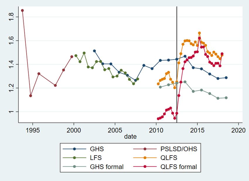
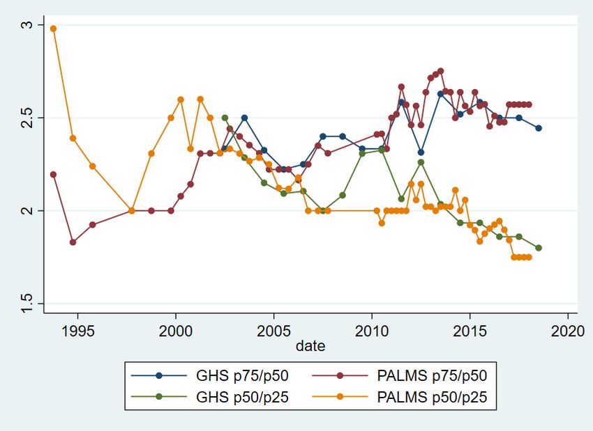
Despite the GHS and QLFS questions asking about gross earnings, it is usually assumed that some
survey respondents report salaries net of some or all deductions. Wittenberg (2014) found
differences between total earnings reported in the QLFS and other firm and national accounts
data. He showed that part of this was due to missing high earners by comparing the QLFS with
tax tables of top earners. Kerr and Wittenberg (2017) showed that total earnings in the LFS and
QLFS were a roughly constant 80 per cent of the national accounts values between 1995 and 2015.
However, Kerr (2020) did find evidence that the QLFS earnings totals as a proportion of the total
labour income reported on IRP5 certificates were declining after 2015.

I follow Wittenberg (2008) and have created bracket weights to adjust for those reporting earnings
in brackets, and I also use a similar method to that used in PALMS for flagging outliers. This
means that earnings in both datasets are as comparable as possible. However, whilst the QLFS
earnings data is imputed, and there are two different imputation approaches (Q1, 2010-Q2, 2012;
Q3, 2012 onwards), the GHS earnings data is not imputed at all. Given the problems with the
QLFS imputations (Kerr and Wittenberg 2021), this suggests that the GHS earnings data will be
more reliable. I investigate this further below.

IRP5 tax certificates are meant to be issued to all employees in IRP5 tax-registered firms who earn
more than ZAR2,000 a year. This means that when comparing earnings in the tax data with the
QLFS or GHS, I should limit the workers in the QLFS and GHS to employees working in tax-
registered firms. Unfortunately, a clear way of doing this is not possible and little information on
employed individuals is available in the GHS compared to the QLFS. In the QLFS, I use the
sample of employees who have a written contract, who are not domestic workers, and who are
either in the public sector or whose employers contribute to the Unemployment Insurance Fund
(UIF) on their behalf. In the GHS, I can only limit to those individuals who report working in the
‘formal sector’, which means that I will be including some self-employed individuals in the formal
sector.

3.3 IRP5 administrative tax data and household survey sample comparisons

Once I undertake the data-cleaning issues discussed above, I should be left with a comparable set
of observations: individuals in the IRP5 data working in the first two weeks of the tax year, and
individuals in the household surveys who, when weighted, represent a comparable set of workers
who would have been issued tax certificates. For the QLFS, I use all four quarters. For the GHS,
there is one survey a year, but the survey is divided into four quarters, and each quarter one of
these groups is surveyed. For the graphical analysis and the inflation adjustments, I assume that
each GHS took place in the middle of the calendar year. Figure 1 shows the number of individuals
in each source of data. The GHS formal sector is much larger than the QLFS formal and IRP5
samples. This means there are several million individuals in the weighted GHS sample who have
not been issued a tax certificate. Unfortunately, this is the best I can do given the covariates present
in the GHS. The QLFS totals look much more comparable.

Figure 1 also shows the fraction of the employed in each QLFS and GHS who have missing
earnings. In the 2010, 2011 and first two quarters of 2012, around 1 per cent of the employed have
missing earnings in the QLFS. This is due to the imputation of all refusals and ‘don’t knows’, as
well as the imputations for bracket responses, discussed above. The GHS missing earnings
percentage calculation includes bracket responses as not having missing earnings. The GHS
earnings data is not imputed and so the proportion of employed with missing earnings is much
higher than the QLFS at the start of the period, but by the end of the period both surveys have
similar proportions of the employed who have missing earnings. This also affects the comparability
of the GHS and QLFS samples. It is not clear why the QLFS proportion with missing earnings
increases substantially around the end of 2015.

 7

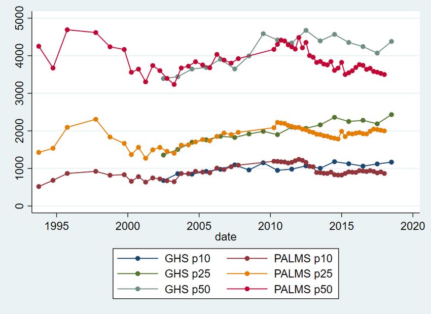
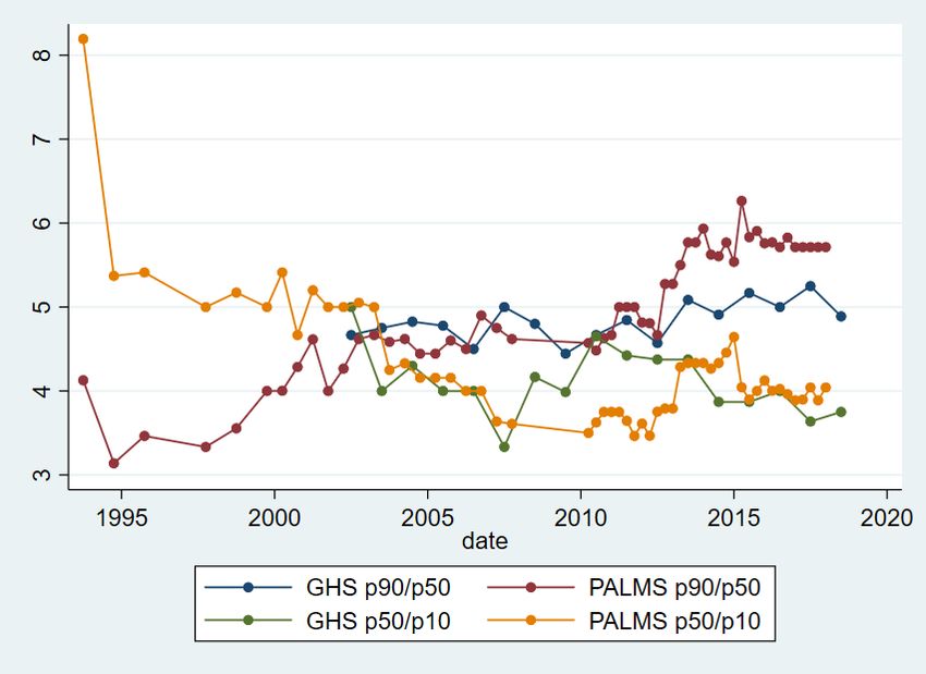
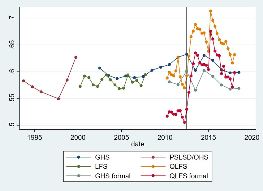
4 Analysis

To begin, I describe changes in earnings inequality in the household survey data. I then contrast
these changes with those estimated using the IRP5 administrative tax data, unearthing several
comparability issues. I then decompose earnings inequality into between- and within-firm
components, allowing comparison of the extent to which differences between firms in South
African contribute to overall earnings inequality.

4.1 Earnings inequality in the QLFS and GHS

Wittenberg (2017) noted that the Gini and other single measures of inequality disguise differential
changes at the top and bottom of the distribution and used percentile ratios to show that, whilst
the 90th and 75th percentiles had moved away from the median, the 10th and 25th percentiles had
moved towards the median. To investigate this further, I first graph actual percentiles and then
percentile ratios. Figures 2 and 3 plot changes in these percentiles. Figure 2 shows that the 25th
percentile and median (to a lesser extent, also the 10th percentile) rose in the mid-1990s but then
declined, and then rose in the 2000s. The trends in the GHS from 2002 onwards and the LFS are
very similar. However, the trends in the GHS and QLFS from 2010 onwards are markedly
different. The median declined for both, although it was a much larger decline in the QLFS. The
25th and 10th percentiles rose for the GHS but declined for the QLFS by around 5 per cent and
25 per cent respectively. This large decline at the bottom of the distribution in the QLFS is
worrying, but the opposite trend in the GHS suggests this may also be a result of the QLFS
imputation methods.

We now use the data from Figures 2 and 3 to graph four percentile ratios, the p90/p50, p50/p10
(Figure 4), p75/p50, and p50/p25 (Figure 5). Figure 4 shows that, in the QLFS, the top of the
distribution has continued to move further away from the middle, and that the bottom has moved
towards the middle, although both have been stable since around 2014. In the GHS, the p90/p50
ratio has increased slightly since 2002, and the p50/p10 ratio has decreased but more erratically.
The 10th percentile ended closer to the median by 2018 than it was in 2002. Figure 5 shows that
the 25th percentile has continued to move closer to the median since around 2000, whilst the 75th
percentile moved away from the median only until around 2011, after which the ratio has been
stable.

Figure 6 shows the Gini coefficient for earnings from 1993 to 2018 using PALMS and the GHS,
whilst Figure 7 shows the variance of log earnings for the same data. Both figures show that the
OHS/LFS and GHS series are stable using both measures of inequality, although the 1993 PSLSD
variance of log earnings is very high. Earnings inequality is extremely high and has shown no sign
of decreasing. As noted by Kerr and Wittenberg (2019a, 2021), the QLFS Gini coefficient trend is
inconsistent with the GHS. The break between the two imputation approaches between Q2 and
Q3 2012 is clearly visible for both measures of inequality. In most of the figures, Q3 and Q4 2012
seem to occupy intermediate positions between the prior and later periods. It is not clear why this
is true.

Figures 6 and 7 also show that earnings inequality is lower when I consider the group of earners
most similar to the SARS data analysed below. In the QLFS, this is employees who are not
domestic workers and whose employers are either in the public sector or deduct UIF. For the
GHS, this is simply workers who report being in the formal sector and who could be wage- or
self-employed. Again, the GHS series is much more stable and credible.

 8

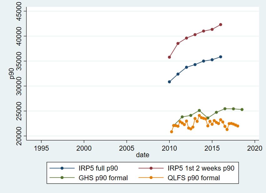
The general finding from the household surveys shown by Wittenberg (2017a, 2017b)—that the
bottom of the earnings distribution was catching up to the middle, and the top of the distribution
was moving away from the middle—has not continued since about 2012, except that the 25th
percentile has continued to move towards the median. Together with the Gini and variance of log
earnings measures, this suggests that, whilst inequality in South Africa is still high, it was stable
from 2012 to 2017. Newer data will show whether this continues to be the case. Before 2012, the
major trends were the movement of the top of the earnings distribution away from the middle,
and the movement of the bottom of the distribution towards the middle.

These inequality estimates rank South Africa as one of the most unequal in the world. Broeke et
al. (2017) showed various inequality measures for gross hourly wages across 29 OECD countries
from two rounds of a comparable survey, the Survey of Adult Skills. The lowest p90/p50 ratio
was 1.56 in Denmark and the highest was 3.33 in Turkey. In the latest GHS, it was 5, whilst it was
just under 6 in the QLFS. The p50/p50 ratio was lowest in Sweden (1.36) and highest in Germany
(2.21) compared to roughly 4 in the GHS and QLFS. For the Gini coefficient, Sweden had the
lowest Gini of 0.17, whilst the highest was 0.44 in Turkey. By contrast, the Gini was 0.6 in the
latest GHS. Fereirra et al. (2017) showed that the Brazilian earnings Gini was 0.5 in 1995 but had
declined to 0.4 in 2012. Thus, whilst there may be some measurement issues in the household
surveys, there is good evidence that South African earnings inequality continues to be amongst the
highest in the world.

The QLFS earnings distribution and associated inequality measures seem less reliable than those
of the GHS. Unfortunately, the GHS has few questions about individual employment, working
conditions, or the individual’s employer. This means it is crucial that unimputed earnings data for
the QLFS is released publicly by Stats SA. In the next section, I describe inequality in earnings
using the IRP5 tax data to examine whether it can shed light on changes in inequality.

4.2 Earnings inequality in the IRP5 data

Household survey data is likely to suffer from under-reporting in earnings, for several reasons.
Participants are asked about gross earnings but may report earnings after deductions such as tax
(Wittenberg 2017c). Rich individuals may be systematically less likely to respond to surveys, in
ways that are not solved by the non-response adjustments undertaken by survey organizations.
And, as I showed earlier, the imputations in the QLFS seem to make inequality measures
unreliable.

It is thus of interest to use the tax data to measure earnings inequality. To do so, I follow the data-
processing suggestions in Kerr (2020). I use data from the 2011–17 tax years. The measure of
earnings I use is derived from the detailed source codes available on each tax certificate rather than
the aggregate earnings variables available in the IRP5 data at the National Treasury data centre,
which incorrectly include some non-labour income. I exclude all certificates with earnings of less
than ZAR2,000 per year (the threshold below which the issuing of certificates is not compulsory)
and with more than ZAR500 million in annual earnings or the equivalent monthly amount. I
calculate monthly earnings from annual earnings using the variables giving the dates employed
from and to on each certificate.

I use two different earnings distributions for the IRP5 data. The first includes only those for the
individuals employed in the first two weeks of the tax year. After dropping certificates where an
individual was not working in the first two weeks of the tax year, I then keep only the highest
certificate for each individual if there is more than one. About 7 per cent of individuals in each tax
year have more than one certificate indicating they worked during the first two weeks.

 9

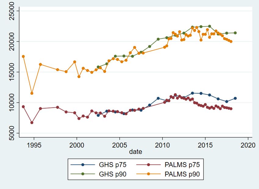
The second distribution is the monthly earnings for all individuals employed throughout the tax
year. I first drop all certificates with earnings of less than ZAR2,000 a year. I then aggregate
earnings for all the remaining certificates for each individual and the length of time they worked
to create a monthly earnings variable for anyone employed throughout the tax year.

The first distribution is conceptually more comparable to the household survey earnings
distributions. The reason for comparability connects to research on employment and earnings
volatility and lifetime earnings inequality, which have received attention in South Africa (Ranchhod
2013; Ranchhod and Dinkelman 2008; Zizzimia and Ranchhod 2020). Kerr (2020) noted that
household surveys ask about earnings for those who worked in the week prior to the interview but
that each year of the IRP5 tax certificate data includes all individuals working at any time during
the year. As it is low-earning individuals who are much less likely to be working throughout the
tax year (Kerr 2018), using tax data for all individuals employed at any point in the year may create
a longer lower tail of the earnings distribution compared to the point-in-time measures from survey
data, all else equal (abstracting from under-reporting and other comparability issues, which I
discuss below). For the same reason, using the household survey earnings data, multiplying
monthly earnings by 12, and using this group of earners employed at a point in time when the
survey was conducted (as in Bassier 2019; Bassier and Woolard 2020; Wittenberg 2017c) may
produce too few earners and a smaller left tail of the survey earnings distribution, if one is
comparing earnings in the household surveys to earnings for anyone employed throughout the
year in the tax data. I investigate this below.

I begin the description of inequality by graphing various percentiles and percentile ratios of
monthly earnings, including the QLFS and GHS for comparison. Figures 8, 9, 10, 11, and 12 show
the 10th, 25th, 50th, 75th, and 90th percentiles, including the survey data used above for
comparison with only the ‘formal sector’ individuals. The QLFS trends are again implausible and,
therefore, I do not spend much time discussing them relative to the tax data. I also show the
percentiles for the tax data sample of individuals employed at any time throughout the tax year.
These are always substantially lower than those for the group of individuals employed only in the
first two weeks of the tax year, reflecting the long lower tail mentioned above.

Figures 8 to 12 show that earnings in the tax data increase at the 10th, 25th, 75th, and 90th
percentiles but not at the 50th (the median). This is very similar to the long-run results shown in
the household surveys by Wittenberg (2017c). Annual growth rates are higher at the 10th and 25th
than at the 75th and 90th percentiles. The GHS shows similar trends for the 10th percentile, the
median, and the 90th percentile but slower growth at the 25th percentile and no growth at the 75th
percentile.

Figures 13 and 14 show variable percentile ratios calculated from Figures 8 to 12. The trends are
similar to those described by Wittenberg (2017a, 2017b). The top part of the earnings distribution
is moving away from the middle, whilst the bottom is catching up the top, or what has been called
wage polarization. These are broadly the same trends as seen in the GHS, but again the QLFS
trends are different and likely less reliable.

Figures 15 and 16 show earnings Gini coefficients and the variance of log earnings for the IRP5
data along with the GHS and QLFS Gini coefficients for formal sector workers only. The Gini
coefficients are extremely high but stable. As expected, the Gini coefficient using only those
working for the first two weeks in the tax year is around 6–7 points lower than when using all
those who worked at any time during the year. There is a sharp decline in inequality between 2012
and 2013, after which inequality is stable. But the variance of log earnings is actually higher when
using only those employed in the first two weeks of the tax year, i.e. not what was expected given
that this excludes a large number of relatively low earners.

 10

The variance of log earnings and the Gini coefficients for the 2011 and 2012 IRP5 data look too
high. This is likely a result of the inclusion of pension and labour income in the source code 3601,
meaning that these years contain perhaps 1.5 million pensioners who are likely to be
disproportionately towards the top of the ‘earnings’ distribution, which pushes up inequality. Kerr
(2018) resolved this issue by excluding around 1.3 million certificates from 23 probable pension
funds in 2011 and 2012. This was not possible in the newer version of the data used for the current
paper. Other researchers have imposed an age cut-off of 60 or 65, which should take care of the
issue of the pensioner category. I have not undertaken that here. Directly identifying individuals
with certificates from pension funds in these two years should be a priority for future versions of
the IRP5 data.

As a result of excluding 2011 and 2012, I can only use five years of data from the 2013–17 tax
years. Earnings inequality was stable over this period when measured by the Gini coefficient and
the variance of log earnings. The GHS shows a similar trend for both these measures, whilst the
QLFS again looks unbelievable. The opposing movements at the top and bottom of the earnings
distribution in the tax data are part of the explanation for this stability.

4.3 Inequality within and between firms

Thus far, I have examined individual-level inequality only. I have shown that earnings inequality is
extremely high and stable. The post-Apartheid trend from the household surveys is that the
bottom of the distribution has moved towards the middle, median real earnings have been roughly
constant, and the top of the earnings distribution has moved away from the middle. The GHS
shows that trend continuing in the most recent five years of data, although the QLFS does not.

The IRP5 data allows a different perspective on earnings inequality because it is possible to know
which firms workers worked in. As discussed in the literature review, this makes it possible to
investigate whether high levels of overall earnings inequality in South Africa occur because all firms
have very high within-firm inequality that mirrors the overall earnings distribution or, alternatively,
whether there may also be large differences in average earnings between firms, and this could
explain some or much of the overall earnings inequality that I showed above. I explore this in two
ways, following Song et al. (2019).

The first method is decomposing the variance in log earnings into two components: the variance
in average (log) earnings differences between firms, and the variance in within-firms (log) earnings.
In the analysis above, I showed that the variance of log earnings in the IRP5 data was stable from
2013 to 2017, although 2011 and 2012 were inconsistent with the estimates.

Following Song et al. (2019) and Alvarez et al. (2018), I write as the log earnings of worker i
in firm j at time t, � as the average earnings at firm j and time t, and � as the average at time t. I
can decompose as:

 = � +( � − � )+ ( - � )

The second term on the right-hand side is the employer deviation and the third is the worker
deviation in the firm. Taking the variance of both sides gives:

 Var( - � )= var( � − � )+ var ( - � )+2Cov( � − � ), - � )

The last term is zero by construction and thus one can simplify and write:

 11

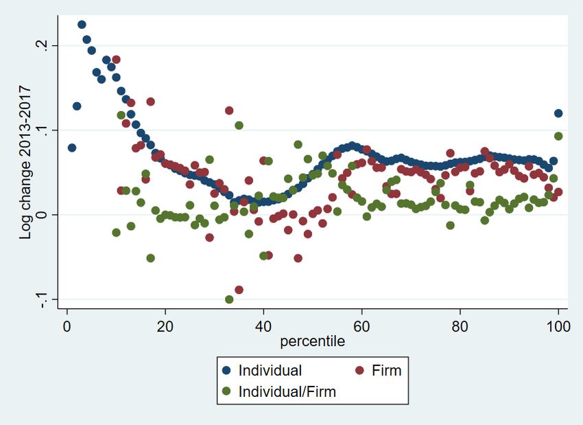
Var( )= var ( � )+ var ( - � )

The two terms on the right-hand side are the variance in average log earnings between firms,
weighted by the number of employees in each firm, and the variance of the difference between
each worker’s log earnings and the average log earnings in their firm.

Table 1 shows this variance decomposition using the 2011–17 tax years. The variation in average
earnings between firms accounts for around 53–58 per cent of overall variance in log earnings,
and thus the variation within firms accounts for around 42–47 per cent of the variance in log
earnings. Lazear and Shaw (2009) found that the between-firm contribution to overall variance in
log earnings was around 20–40 per cent in nine European countries and the USA. Song et al.
(2019) found that it was 42 per cent in 2013, and Alvarez et al. (2018) found that it was an average
of 66 per cent between 1996 and 2012 in Brazil. Thus, average differences between firms in South
Africa account for more of the overall variance in log earnings than in this sample of developed
countries, but substantially less than in Brazil. Song et al. (2019) found that between-firm inequality
in the USA rose due to sorting and segregation of workers: high-earning workers increasingly
worked in high-wage firms and high-earning workers increasingly worked with each other. Bassier
(2019) provided evidence for sorting in South Africa in which high-wage workers were very likely
to work at firms with high rents.

As Song et al. (2019) pointed out, and as the analysis plotting various percentiles showed above,
the variance of log earnings does not allow for trends in inequality over time to vary across the
distribution. To investigate this further, using the firm data, I plot three different graphs in Figure
17. The first is the change in average earnings between 2013 and 2017 at each percentile of the
individual earnings distribution. 3 Similar to what I showed for five percentiles above, I plot average
changes in earnings between 2013 and 2017 at each percentile. This shows more fully that the
bottom 10 per cent experienced the largest changes in earnings, the middle of the distribution
experienced almost no change in earnings, and the top 35 per cent experienced similar growth of
around 0.6 per cent a year. The 99th percentile is different: real earnings grew around 10 per cent
or around 1.6 per cent a year.

The red dots show the changes in average earnings for the firms employing workers in each
percentile. 4 As the red dots track the blue ones closely, this means that the earnings of individuals’
co-workers tracked their own at most parts of the distribution. The bottom 10 per cent looks odd,
perhaps due to coverage changes. The earnings of the individuals at the top 2 percentiles grew
faster than those of their co-workers. The green dots are the residual, i.e. they indicate the
difference between the individual and average firm growth at each earnings percentile. As they are
generally close to zero, this indicates again that the earnings of individuals’ co-workers broadly
tracked individuals’ own earnings for most percentiles, other than at a few percentiles at the bottom
and the top 1 per cent. The broad conclusion one can draw from Figure 14 is thus that within-
firm inequality did not change very much, as the variance decomposition above also showed.

3
 I do not use 2011 and 2012 given the comparability issues shown above.
4
 I do not include the firm and residual changes for the bottom 10 percentiles because the firm changes are extremely
large and that obscures the trends for the rest of the distribution.

 12

5 Conclusions

The levels of income and earnings inequality in South Africa are amongst the highest in the world.
In this paper, I documented that this has remained true throughout the post-Apartheid period,
using household survey and administrative tax data. Using the labour market data in PALMS from
1993 to around 2012, the relative stability of two of the measures of inequality that I used—the
variance of log earnings and the Gini coefficient—hid more complex trends. The bottom of the
earnings distribution caught up to the median, median real earnings were roughly constant, and
the top of the distribution moved away from the median, a phenomenon first shown by Wittenberg
(2017a, 2017b).

From 2012, there are several oddities that deserve further scrutiny. The QLFS earnings
imputations result in unreliable trends in the Gini coefficient, the variance of log earnings, and the
five percentiles I have shown. The GHS earnings data seems more reliable. It shows that the Gini
and variance of log earnings were stable from the early 2000s up until 2018. But the trends of the
bottom catching up to the middle of the distribution, and the top moving away from the middle,
are not as strong in the GHS as in the IRP5 tax data. Given the problems with the QLFS earnings
data, discussed in more detail in Kerr and Wittenberg (2021), it seems crucial that Stats SA releases
unimputed QLFS earnings data. This has now occurred for 2020 Q2, although what is really
needed is a rerelease of unimputed earnings data from 2009 Q3 until the present and ongoing
timely releases as future surveys are conducted.

As well as providing a useful alternative measure of earnings growth and inequality to the
household surveys, the IRP5 data allows for a decomposition of inequality focusing on the firm.
Differences in average earnings between firms are higher than in developed countries, although
lower than in Brazil. This is an interesting and fruitful area for further research.

The broad conclusion from this paper is that earnings inequality is extremely high and has not
come down. The recent trends in earnings equality are not so clear, partly due to earnings data
issues in the QLFS household surveys. Newer and more reliable data from household surveys and
the SARS tax data should shed light on the recent trends in earnings inequality.

References

Abowd, J.M., F. Kramarz, and D.N. Margolis (1999). ‘High Wage Workers and High Wage
 Firms’. Econometrica, 67(2): 251–333.
Acemoglu, D., and D. Autor (2011). ‘Skills, Tasks and Technologies: Implications for Employment and
 Earnings’. In O. Ashenfelter and D. Card (eds), Handbook of Labor Economics Volume 4. Amsterdarm:
 Elsevier. https://doi.org/10.1016/S0169-7218(11)02410-5
Alvarez, J., F. Benguria, N. Engbom, and C. Moser (2018). ‘Firms and the Decline in Earnings Inequality
 in Brazil’. American Economic Journal: Macroeconomics, 10(1): 149–89.
 https://doi.org/10.1257/mac.20150355
Bassier, I. (2019). ‘The Wage-setting Power of Firms: Rent-sharing and Monopsony in South
 Africa’. WIDER Working Paper 2019/34. Helsinki: UNU-WIDER.
 https://doi.org/10.35188/UNU-WIDER/2019/668-5
Bassier, I., and I. Woolard (2020). ‘Exclusive Growth? Rapidly Increasing Top Incomes Amid Low National
 Growth in South Africa’. South African Journal of Economics, (Early View).
 https://doi.org/10.1111/saje.12274

 13

Bhorat, H., K. Lilenstein, M. Oosthuizen, and A. Thornton (2020). ‘Wage Polarization in a High-Inequality
 Emerging Economy: The Case of South Africa’. WIDER Working Paper 2020/55. Helsinki: UNU-
 WIDER. https://doi.org/10.35188/UNU-WIDER/2020/812-2
Bhorat, H., M. Oosthuizen, K, Lilenstein, and F. Steenkamp (2017). ‘Firm-level Determinants of Earnings
 in the Formal Sector of the South African Labour Market’. WIDER Working Paper 2017/25, Helsinki:
 UNU-WIDER. https://doi.org/10.35188/UNU-WIDER/2017/249-6
Broeke, S., G. Quintini, and M. Vandeweyer (2017). ‘Explaining International Differences in Wage
 Inequality: Skills Matter’. Economics of Education Review, 60: 112–24.
 https://doi.org/10.1016/j.econedurev.2017.08.005
Cassim, A., and D. Casale (2018). ‘How Large is the Wage Penalty in the Labour Broker Sector?’. WIDER
 Working Paper 2018/48, Helsinki: UNU-WIDER.
 https://doi.org/10.35188/UNU-WIDER/2018/490-2
Docrat, F. (2017). ‘Must Outsourcing Fall? an Estimation of the Outsourcing Wage Penalty for Guards and
 Cleaners in Post-apartheid South Africa’. Unpublished University of Cape Town Honours Economics
 Long Paper. Cape Town: University of Cape Town.
Ebrahim, A., and C. Axelson (2019). ‘The Creation of an Individual Panel Using Administrative Tax
 Microdata in South Africa’. UNU-WIDER Working Paper, 2019-27. Helsinki: UNU-WIDER.
 https://doi.org/10.35188/UNU-WIDER/2019/661-6
Finn, A., and M. Leibbrandt (2018). ‘The Evolution and Determination of Earnings Inequality in Post-
 Apartheid South Africa’. WIDER Working Paper 2018/83. Helsinki: UNU-WIDER.
 https://doi.org/10.35188/UNU-WIDER/2018/525-1
Finn, A., and V. Ranchhod (2017). ‘Short-run Differences Between Static and Dynamic Measures of
 Earnings Inequality in South Africa’. REDI3x3 Working Paper 35. Cape Town: The Research Project
 on Employment, Income Distribution and Inclusive Growth.
Hirsch, B.T., and E.J. Schumacher (2004). ‘Match Bias in Wage Gap Estimates Due to Earnings
 Imputation’. Journal of Labor Economics, 22(3): 689–722. https://doi.org/10.1086/383112
Kerr, A. (2018). ‘Job Flows, Worker Flows and Churning in South Africa’. South African Journal of
 Economics, 86(S1): 141–66. https://doi.org/10.1111/saje.12168
Kerr, A. (2020). ‘Earnings in the South African Revenue Service IRP5 data’. WIDER Working Paper
 2020/62. Helsinki: UNU-WIDER. https://doi.org/10.35188/UNU-WIDER/2020/819-1
Kerr, A., D. Lam, and M. Wittenberg (2019). ‘Post-Apartheid Labour Market Series [dataset]’. Version 3.3.
 Cape Town: DataFirst (producer and distributor).
Kerr, A., and M. Wittenberg (2017). ‘Public Sector Wages and Employment in South Africa’. SALDRU
 Working Paper 214. Cape Town: SALDRU, University of Cape Town.
Kerr, A., and M. Wittenberg (2019a). ‘Earnings and Employment Microdata in South Africa’. WIDER
 Working Paper 2019/47. Helsinki: UNU-WIDER.
 https://doi.org/10.35188/UNU-WIDER/2019/681-4
Kerr, A., and M. Wittenberg (2019b). ‘A Guide to PALMS version 3.3’. Available at:
 https://www.datafirst.uct.ac.za/dataportal/index.php/catalog/434/download/10286 (accessed 13
 April 2021).
Kerr, A., and M. Wittenberg (2021). ‘Union Wage Premia and Wage Inequality in South Africa’. Economic
 Modelling, 97: 255–71. https://doi.org/10.1016/j.econmod.2020.12.005
Lazear, E. and K. Shaw (2009). ‘Wage Structure, Raises and Mobility: An Introduction to International
 Comparisons of the Structure of Wages Within and Across Firms’. In E. Lazear and K. Shaw (eds),
 The Structure of Wages: An International Comparison. Cambridge, MA: NBER.
Leibbrandt, M., I. Woolard, A. Finn, and J. Argent (2010). ‘Trends in South African Income Distribution
 and Poverty Since the Fall of Apartheid’. OECD Social, Employment and Migration Working Papers
 101. Paris: OECD Publishing. https://doi.org/10.1787/5kmms0t7p1ms-en

 14

Lemieux, T. (2006). ‘Increasing Residual Wage Inequality: Composition Effects, Noisy Data, or Rising
 Demand for Skill?’. American Economic Review, 96(3): 461–98. https://doi.org/10.1257/aer.96.3.461
National Treasury and UNU-WIDER (2019) ‘IRP5 2008–2017’ [dataset]. Version 0.6. Pretoria: South
 African Revenue Service [producer of the original data], 2018. Pretoria: National Treasury and UNU-
 WIDER [producer and distributor of the harmonized dataset], 2019.Ranchhod, V. (2013). ‘Earnings
 Volatility in South Africa’. SALDRU Working Paper 121. Cape Town: SALDRU, University of Cape
 Town.
Ranchhod, V., and T. Dinkelman (2008). ‘Labour Market Transitions in South Africa: What Can we Learn
 from Matched Labour Force Survey Data?’. SALDRU Working Paper 14. Cape Town: SALDRU,
 University of Cape Town.
Redonda, A., and C. Axelson (2021). ‘Assessing Pension-Related Tax Expenditures in South Africa.
 Evidence from the 2016 Retirement Reform’. WIDER Working Paper 2021/54. Helsinki: UNU-
 WIDER. https://doi.org/10.35188/UNU-WIDER/2021/992-1
Song, J., D.J. Price, F. Guvenen, N. Bloom, and T. von Wachter (2019). ‘Firming up Inequality’. The
 Quarterly Journal of Economics, 134(1): 1–50. https://doi.org/10.1093/qje/qjy025
Statistics South Africa (2002–18). ‘General Household Surveys’. Available through DataFirst at:
 https://www.datafirst.uct.ac.za/dataportal/index.php/catalog/central#_r=1612534493386&collecti
 on=&country=&dtype=&from=1947&page=1&ps=&sk=GHS&sort_by=nation&sort_order=&to
 =2020&topic=&view=s&vk= (accessed 12 January 2021).
Tregenna, F. (2010). ‘How Significant is Intersectoral Outsourcing of Employment in South
 Africa?’. Industrial and Corporate Change, 19(5): 1427–57. https://doi.org/10.1093/icc/dtq001
Wittenberg, M. (2008). ‘Nonparametric Estimation When Income is Reported in Bands and at Points’.
 Economic Research Southern Africa Working Paper 94. Cape Town: ERSA.
Wittenberg, M. (2014). ‘Analysis of Employment, Real Wage, and Productivity Trends in South Africa Since
 1994’’. Conditions of Work and Employment Series 45. Geneva: International Labour Organisation.
Wittenberg, M. (2017a). ‘Wages and Wage Inequality in South Africa 1994–2011: Part 1–Wage
 Measurement and Trends’. South African Journal of Economics, 85(2): 279–97.
 https://doi.org/10.1111/saje.12148
Wittenberg, M. (2017b). ‘Wages and Wage Inequality in South Africa 1994–2011: Part 2–Inequality
 Measurement and Trends’. South African Journal of Economics, 85(2): 298–318.
 https://doi.org/10.1111/saje.12147
Wittenberg (2017c). ‘Measurement of Earnings: Comparing South African Tax and Survey Data’. REDI3x3
 Working Paper 41. Cape Town: SALDRU, University of Cape Town.
Zizzamia, R., and V. Ranchhod (2020). ‘Earnings Inequality Over the Life-course in South Africa’. AFD
 Research Paper number 160. Paris: AFD.

 15