Mapping seasonal glacier melt across the Hindu Kush Himalaya with time series synthetic aperture radar (SAR)

Page created by Earl Alexander
 
CONTINUE READING
Mapping seasonal glacier melt across the Hindu Kush Himalaya with time series synthetic aperture radar (SAR)
The Cryosphere, 15, 4465–4482, 2021
https://doi.org/10.5194/tc-15-4465-2021
© Author(s) 2021. This work is distributed under
the Creative Commons Attribution 4.0 License.

Mapping seasonal glacier melt across the Hindu Kush
Himalaya with time series synthetic aperture radar (SAR)
Corey Scher1,2 , Nicholas C. Steiner2 , and Kyle C. McDonald1,2,3
1 Department of Earth and Environmental Sciences, The Graduate Center,
City University of New York, New York, NY 10031, USA
2 Department of Earth and Atmospheric Sciences, The City College of New York,

City University of New York, New York, NY 10031, USA
3 Carbon Cycle and Ecosystems Group, Jet Propulsion Laboratory, California Institute of Technology,

4800 Oak Grove Drive, Pasadena, CA 91001, USA

Correspondence: Nicholas C. Steiner (nsteiner@ccny.cuny.edu)

Received: 29 June 2020 – Discussion started: 3 September 2020
Revised: 24 June 2021 – Accepted: 11 July 2021 – Published: 24 September 2021

Abstract. Current observational data on Hindu Kush Hi-           glacier surface melt and the development and assessment of
malayas (HKH) glaciers are sparse, and characterizations of      surface energy balance models of melt-driven ablation across
seasonal melt dynamics are limited. Time series synthetic        the global cryosphere.
aperture radar (SAR) imagery enables detection of reach-
scale glacier melt characteristics across continents. We an-
alyze C-band Sentinel-1 A/B SAR time series data, com-
prised of 32 741 Sentinel-1 A/B SAR images, and determine        1   Introduction
the duration of seasonal glacier melting for 105 432 mapped
glaciers (83 102 km2 glacierized area, defined using optical     Global warming driven by the anthropogenic release of ge-
observations) in the HKH across the calendar years 2017–         ologic carbon is causing mass loss of alpine glaciers world-
2019. Melt onset and duration are recorded at 90 m spatial       wide (Brangers et al., 2020; Zemp et al., 2006). The Hindu
resolution and 12 d temporal repeat. All glacier areas within    Kush Himalaya (HKH) region, known colloquially as the
the HKH exhibit some degree of melt. Melt signals persist for    “Third Pole,” has the most ice-covered area on Earth after
over two-thirds of the year at elevations below 4000 m a.s.l.    the high-latitude polar regions (Yao et al., 2012). In con-
and for nearly half of the calendar year at elevations exceed-   trast to large ice sheets near the poles, these relatively small
ing 7000 m a.s.l. Retrievals of seasonal melting span all ele-   alpine glaciers – perched at some of the highest elevations
vation ranges of glacierized area in the HKH region, extend-     on Earth – are among the most sensitive indicators within the
ing greater than 1 km above the maximum elevation of an          global cryosphere of changes in global climate (Anthwal et
interpolated 0 ◦ C summer isotherm and at the top of Mount       al., 2006). Just as the recession of these sensitive mountain
Everest, where in situ data and surface energy balance mod-      glaciers contributes to over one-quarter of global sea level
els indicate that the Khumbu Glacier is melting at surface air   rise (Zemp et al., 2019), disturbances accompanying HKH
temperatures below −10 ◦ C. Sentinel-1 melt retrievals reflect   glacier retreat pose innumerable hazards to humans and nat-
broad-scale trends in glacier mass balance across the region,    ural ecosystems. Glacier retreat threatens to disturb the dy-
where the duration of melt retrieved in the Karakoram is on      namics of river systems delivering freshwater resources to
average 16 d less than in the eastern Himalaya sub-region.       nearly 2 billion people across South and Central Asia (Brown
Furthermore, percolation zones are apparent from meltwa-         et al., 2007; Milner et al., 2017). Outburst floods resulting
ter retention indicated by delayed refreeze. Time series SAR     from glacier mass loss have killed at least 6300 people in
datasets are suitable to support operational monitoring of       the Himalayas alone and have caused extensive damage to
                                                                 property and livelihoods. These outbursts are expected to in-

Published by Copernicus Publications on behalf of the European Geosciences Union.
Mapping seasonal glacier melt across the Hindu Kush Himalaya with time series synthetic aperture radar (SAR)
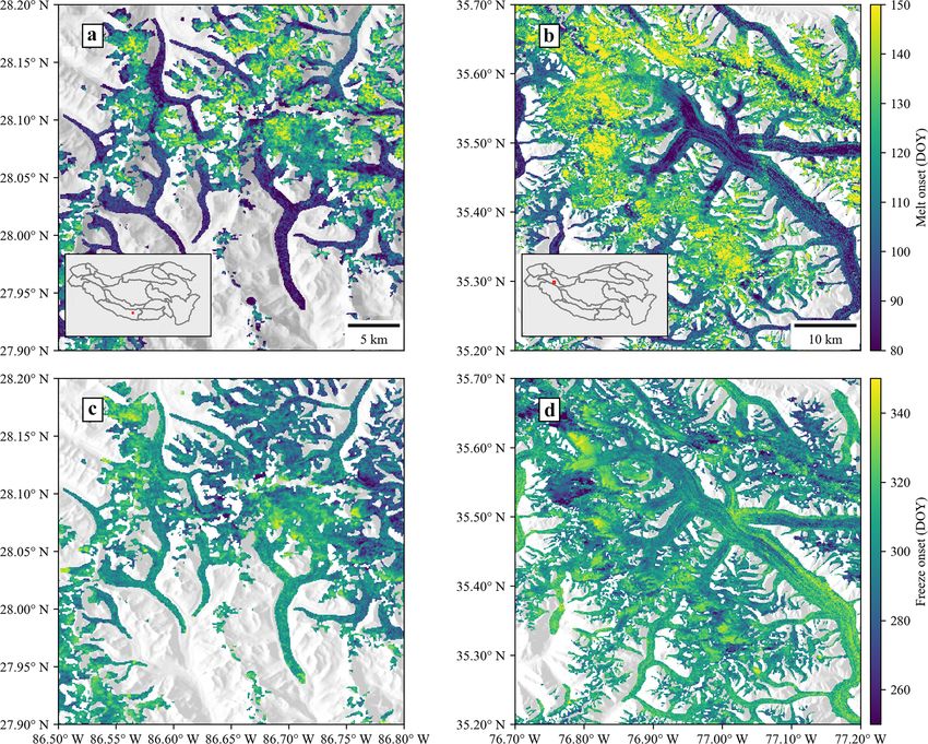
4466                                      C. Scher et al.: Mapping seasonal glacier melt across the Hindu Kush Himalaya

crease in frequency with continued glacier wasting (Carriv-       balance is necessary to capture seasonal and regional vari-
ick and Tweed, 2016). Some organisms endemic to alpine            ability in glacier wasting across the HKH during melt–freeze
aquatic ecosystems may become extinct as they lose biogeo-        cycles.
chemical regulation from upstream glaciers (Jacobsen et al.,
2012). As global temperatures rise, and perennial snow and        Snowmelt detection and radar imaging
ice cover decreases, societies are faced with difficult deci-
sions around the costs and benefits of adapting to a chang-       This study builds on extensive research on microwave scat-
ing climate within and around the HKH region (Brown et            tering from dry and wet snow and associated techniques for
al., 2007). Informed decision-making for successful climate       snowmelt retrieval from imaging radar data to present an
change adaptation will require knowledge of the state of nat-     operational monitoring system for spatially resolved glacier
ural systems and how these systems are projected to change        surface melt characteristics using synthetic aperture radar
alongside future increases in population and global average       (SAR) time series and outlines of glacier area derived from
temperature (Bogardi et al., 2012).                               satellite optical imagery across the HKH. Microwave re-
   Substantial uncertainties exist in projected disturbances      mote sensing has been used to reliably monitor melt pat-
associated with a changing climate, environment and hydro-        terns across glaciers and ice sheets (Abdalati and Steffen,
logic regime across the greater Himalayas due in part to a        2001; Ashcraft and Long, 2007; Jezek et al., 1994b; Steiner
lack of observations of in situ hydrology and meteorology at      and Tedesco, 2014). Because imaging radar is independent
high elevations (Hock et al., 2019; Litt et al., 2019; Marzeion   of solar illumination and largely unaffected by cloud cover
et al., 2020). The magnitude and rate of ablation from surface    and atmospheric conditions, the fidelity of radar observa-
melting is of particular importance as it drives changes in       tions is defined by the frequency of the satellite platform’s
accumulation-zone snow-properties, such as percolation and        observational opportunities and by the characteristics of the
densification, that feed back into increased melting (Alexan-     imaging sensor. At C-band frequencies, frozen glacier per-
der et al., 2019). Surface melting has also been linked to        colation areas are recognized as one of the brightest radar
increased englacial temperatures, resulting in faster ice mo-     targets on Earth, and glacier surfaces are unambiguous tar-
tion (Miles et al., 2018). Although the general trajectory of     gets for determination of the melting or frozen state of the
changes to the HKH cryosphere is understood (i.e., acceler-       surface (melt/freeze) characteristics (Jezek et al., 1994; Rott
ated glacier mass loss on a decadal scale in the central and      and Mätzler, 1987). Detection of seasonal melt on ice sur-
eastern Himalaya) (Fujita and Nuimura, 2011), a consensus         faces at C-band frequencies (4–8 GHz) depends on a strong
in projecting changes to HKH hydrology is lacking largely         radiometric response at melt onset (MO), when liquid water
because of missing in situ snow and ice monitoring data           content introduced to an otherwise frozen snow or firn ma-
across these glaciated river basins (Marzeion et al., 2020).      trix causes a drastic decrease in the radar backscatter from
However, construction and maintenance of in situ monitor-         the medium (Hallikainen et al., 1986). Deep, frozen snow
ing station networks are costly and labor-intensive because of    and firn have a high scattering albedo across microwave fre-
the complexity of the high-mountain glaciated terrain. Satel-     quencies (Matzler, 1998), resulting in high radar backscat-
lite imaging radar retrieval of alpine glacier melt character-    ter intensity over glaciated regions during the frozen months
istics has long been proposed as a source of data for hydro-      (Winsvold et al., 2018; Wiscombe and Warren, 1980). The
logic and glaciologic research (Shi et al., 1994). Understand-    introduction of liquid water in the snow or firn matrix at
ing of surface melting from observation records will enable       even hydrologically minimal amounts causes a pronounced
advanced climate change projections of glacier wasting that       increase in the medium’s dielectric constant, increasing radar
require snow property dynamics describing the retention, re-      signal attenuation and diminishing volume scattering and
freezing and drainage of liquid water within glacier snow and     leading to a pronounced decrease in radar backscatter, usu-
firn (Pritchard et al., 2020).                                    ally by half power or more (Kendra et al., 1998; Shi and
   Recent findings indicate that shortwave radiation drives       Dozier, 1995). In areas that are seasonally snow-free, e.g., for
melting at elevations where air temperatures are perenni-         glacier ablation areas of debris cover or bare ice, melting
ally below freezing, such as those on Mount Everest, where        conditions are dominated by heterogeneous scattering mech-
temperatures never exceed −10 ◦ C (Matthews et al., 2019,         anisms following the disappearance of seasonal snow, a topic
2020). These in situ findings indicate the degree to which        of study not well represented in the theoretical literature
temperature-indexed melt models are underestimating abla-         on radar physics, likely due to the complex nature of the
tion at these elevations using a 0 ◦ C threshold for glacier      glacier ablation surface. Because of the relatively strong sig-
melting. Further, studies of glacier wasting in High Moun-        nal produced at the onset of melting, radar-based melt de-
tain Asia have shown variability in patterns and magnitude        tection records have been developed across regions of the
of glacier wasting across sub-regions of the HKH that would       global cryosphere for several decades using both real and
be difficult to capture in numerical models using degree-day      synthetic aperture radar sensors (Bhattacharya et al., 2009;
assumptions (Brun et al., 2017). An observationally based         Bindschadler et al., 1987; Koskinen et al., 1997). Subse-
dataset providing characteristics of the glacier surface energy   quently, snowmelt detection algorithms have been developed

The Cryosphere, 15, 4465–4482, 2021                                                  https://doi.org/10.5194/tc-15-4465-2021
Mapping seasonal glacier melt across the Hindu Kush Himalaya with time series synthetic aperture radar (SAR)
C. Scher et al.: Mapping seasonal glacier melt across the Hindu Kush Himalaya                                               4467

using a host of radar sensors to monitor the onset and du-         methods often employed for glaciers and ice sheets. In this
ration of snowmelt across glaciers and ice sheets (Abdalati        paper we utilize SAR data to retrieve melt status on HKH
and Steffen, 2001; Ashcraft and Long, 2007; Bahr et al.,           glacier surfaces with a simple threshold-based change de-
1997; Jezek et al., 1994; Kayastha et al., 2020; Koskinen          tection classification of the binary melt/freeze state of the
et al., 1997; Winebrenner et al., 1994). Prior applications of     surface – an observational constraint on glacier ablation. It
SAR mapping of seasonal surface melting over ice sheets and        is possible that intense incident solar radiation is driving
glaciers have been limited by a lack of repeat observations        these melt processes at elevations above the 0 ◦ C summer
such as those now available from the Sentinel-1 SAR con-           isotherm (Matthews et al., 2019) across the entirety of the
stellation (Lund et al., 2019).                                    HKH and that the sensitivity of SAR backscatter to changes
   Observations from time series SAR data have been used           in the glacier surface melt/freeze condition as seen when wa-
to delineate zones of glacier facies and regions of glacier        ter transitions between solid and liquid phases provides a real
mass balance (Winsvold et al., 2018). In glacier percolation       alternative to temperature–elevation lapse rate estimates of
zones, seasonally wet snow refreezes into ice lenses, pipes,       melting (Litt et al., 2019) for assessing models of glacier ab-
and other percolation-related features that amplify both sur-      lation. Though coarse in temporal resolution relative to typ-
face and volume scattering of C-band radar and result in the       ical meteorological datasets, retrieval of melt status using
brightest SAR backscatter being captured during the frozen         SAR time series produces mappings with very high spatial
periods (Jezek et al., 1994; Rau et al., 2000). Studies have       resolution and a continuous record of melt timing and dura-
shown that SAR backscatter generally increases with eleva-         tion across glaciated regions. We present an application of
tion across glacier surfaces during frozen periods, from the       this melt retrieval technique at the scale of the HKH with
glacier terminus, through zones of ablation and frozen melt-       spatiotemporal fidelity adequate for capturing seasonal vari-
water percolation, and eventually attenuating in zones where       ability in melt timing and duration across individual glacier
dry snow accumulates (Winsvold et al., 2018). In transitions       surfaces and sub-regional heterogeneities across the HKH.
between these zones there are pronounced backscatter con-
trasts rather than smooth, gradual transitions. At C-band fre-
quencies, radar scattering within glacier percolation areas
dominates the backscatter amplitude during frozen periods          2   Setting and data
(Jezek et al., 1994). Importantly for melt retrievals, the di-
minished volume scattering during surface melting in areas         The HKH region (Fig. 1) spans 4.2 × 10⁶ km2 , including
of meltwater percolation creates a pronounced and unam-            areas inhabited by 240 million people, with nearly 2 bil-
biguous radar signature in time series observations. The sen-      lion people relying on the delivery of water resources from
sitivity of SAR backscatter to the introduction of liquid water    catchments that originate within the region (Scott et al.,
in an otherwise frozen snowpack or firn structure provides a       2019). Within the high-elevation HKH, seasonal meltwater
reliable mechanism for the retrieval of percolation zone melt      from snow and glacier ice is the primary source of domes-
characteristics (Lievens et al., 2019). In refreezing percola-     tic freshwater supply (Bolch et al., 2012). Wasting of HKH
tion zones, the upper layers of firn will freeze first, with the   glaciers poses a risk to the domestic water resource sup-
freezing front advancing downward across layers, thus pro-         ply for those populations living within these high-elevation
gressively increasing backscatter and with decreasing total-       HKH catchments (Wood et al., 2020). Glacier wasting in the
column liquid water content (Ashcraft and Long, 2005). In          HKH is heterogeneous, and the increase in global average
this way, the timing of refreeze relative to the surface en-       temperature has caused mass wasting of mountain glaciers
ergy balance at the surface provides a direct and spatially re-    across all HKH sub-regions (Farinotti et al., 2020; Gardelle
solved indicator of subsurface meltwater storage within the        et al., 2012). Distinct glacio-climatic sub-regions are charac-
snow or firn and delineates the percolation zones over moun-       terized by these unique dynamics of glacier wasting (Bolch
tain glaciers. Like in the accumulation zone, the surface melt-    et al., 2019a). The wasting of HKH glaciers is thus a spa-
ing response in the ablation zone will dominate the seasonal       tially and temporally heterogeneous phenomenon where dis-
trends in backscatter because of absorption from liquid water      tinct glacio-climatic regimes control ablation (Bolch et al.,
at the surface over both bare-ice and debris-covered portions      2012). In this study, we refer to glacio-climate sub-regions
of ablation areas. Although the absolute fraction of backscat-     delineated in Bolch et al. (2019a) and modified by Shean
ter at C-band frequencies over debris-covered portions of ab-      et al. (2020). These delineations of glacio-climate were pro-
lation zones attributed to volume scatter is not well known,       duced by the Hindu Kush Himalaya Monitoring and Assess-
there is evidence that for low frequencies it can account for a    ment Program (HiMAP), and we refer to the sub-regional
majority of radar observations (Huang et al., 2017).               delineations as “HiMAP regions” throughout the text. We se-
   This study enlists SAR data acquired at a spatiotempo-          lected 12 HiMAP sub-regions that intersected with a bound-
ral resolution that captures melt variability across mountain      ary of the HKH region delineated by the International Cen-
glacier surfaces suitable for constraining seasonal character-     tre for Integrated Mountain Development (ICIMOD, 2008).
istics of melt onset and duration while building on associated     The HKH region, HiMAP sub-regions and glaciated area

https://doi.org/10.5194/tc-15-4465-2021                                                 The Cryosphere, 15, 4465–4482, 2021
Mapping seasonal glacier melt across the Hindu Kush Himalaya with time series synthetic aperture radar (SAR)
4468                                      C. Scher et al.: Mapping seasonal glacier melt across the Hindu Kush Himalaya

summaries within each HiMAP sub-region are illustrated in         and duration. Cross-polarized SAR backscatter provides en-
Fig. 1 alongside the Sentinel-1 acquisition plan.                 hanced observational sensitivity to volume scattering of the
                                                                  radar signal in deep, dense and weathered snowpack and firn
2.1    GAMDAM glacier inventory (GGI)                             (Rott and Mätzler, 1987). We selected cross-polarized (VH)
                                                                  Sentinel-1 A/B observations because VH data show less an-
The Glacier Area Mapping for Discharge from the Asian             gular sensitivity to contrasts between dry and wet snow (Na-
Mountains (GAMDAM) glacier inventory (GGI) is a con-              gler et al., 2016). Cross-polarized Sentinel-1 SAR did not
temporary (July 2019) database on glacier outlines for the        become available over the HKH until early 2017 and thus re-
region of High Mountain Asia (Fig. 1). These outlines were        stricted the timeframe of this study. As illustrated in Fig. 2,
originally delineated automatically using cloud- and snow-        we observe a large (>3 dB) difference in the seasonal radar
free satellite optical imagery in an initial release of the       backscatter between frozen and melting periods across most
database (Nuimura et al., 2015). As a recent update to the        glacier surfaces in cross-polarized (VH) SAR data.
database, each outline was individually inspected for qual-
ity control to correct discrepancies where automatic glacier      2.3   Computing infrastructure
delineation lost accuracy in terrain-occluded areas, at debris-
covered portions of glaciers and through obstruction under        A cloud-computing platform and application programming
seasonal snowpack. The recently updated glacier outlines          interface (Google Earth Engine) with pre-processed radio-
were derived from satellite optical imagery captured across       metrically terrain-corrected Sentinel-1 A/B data were used to
the HKH by Landsat 5 and 7 between 1990–2010 (Sakai,              detect melt characteristics across the region (Gorelick et al.,
2019). Although these data are the most current in terms of       2017). Radiometric terrain correction of Sentinel-1 data was
quality control spanning the study region, they do not neces-     conducted upon ingestion to the cloud server using the ESA’s
sarily capture debris-covered portions of glaciers due to con-    method contained within the Sentinel Applications Platform
fusion with land in optical image classification schemes, an      (SNAP) processing toolbox. The SNAP toolbox is used for
issue that may be resolved with interferometric SAR phase         Sentinel-1 images to update orbit metadata with restituted or-
decorrelation (Bolch et al., 2019b). The 2018 GAMDAM              bit files, remove invalid edge data and low-intensity noise, re-
database contained within the HiMAP sub-regions includes          move thermal noise, compute σ 0 backscatter, and conduct or-
105 432 distinct glacier outlines, spanning a total area of       thorectification upon ingestion of data to the server (Google,
83 102 km2 within the HKH (Nuimura et al., 2015).                 2020). The SNAP toolbox terrain correction functionality
                                                                  utilizes the 30 m spatial resolution SRTM DEM (Farr, 2007;
2.2    Sentinel-1 synthetic aperture radar                        Margulis et al., 2019). The pre-processed SAR time series
                                                                  data and application programming interface (API) function-
The Sentinel-1 A/B satellites were launched in April of 2014      ality used to derive glacier melting characteristics are avail-
and 2016, respectively, and collect C-band (5.405 GHz) SAR        able from Google Earth Engine and can be used to recreate
data with a combined revisit interval of 6 d over of the ma-      the work presented in this study.
jority of the terrestrial Earth. Each Sentinel-1 scene acquired
in the interferometric wide-swath (IW) mode has a width           2.4   Automated weather station data
of 250 km and a resolution of 5 × 20 m in range and az-
imuth at the Equator. This study utilized images taken in         Measurements from two automated weather stations (AWSs)
the IW mode and in a cross-polarized state (VH). Sentinel-        are used to estimate surface energy balance (SEB) and eval-
1 data were accessed through a cloud-computing platform           uate surface melting conditions over the Khumbu Glacier,
(discussed below), wherein SAR scenes were radiometrically        and measurements from two additional AWSs are used to
terrain-corrected to sigma naught backscatter coefficients in     calculate temperature–elevation lapse rates for comparison
decibels (dB) using the European Space Agency’s (ESA)             with melt retrievals (Table 2). The Camp and the South Col
Sentinel Application Platform (SNAP) toolbox and the Shut-        AWSs were installed around Mount Everest, Nepal, as part
tle Radar Topography Mission (SRTM) 30 m digital eleva-           of the National Geographic and Rolex Perpetual Planet Ex-
tion model (DEM) (Farr, 2007) upon ingestion into the cloud       pedition to Mt. Everest in April–May 2019 (Matthews et al.,
environment. Data from both the ascending- and descending-        2019). Measurements were collected at an hourly interval
orbit nodes were analyzed across the study region for a total     and include air temperature, wind speed, relative humidity,
consideration of 32 741 individual Sentinel-1 A/B IW scenes       incoming shortwave and longwave radiation, and baromet-
across 46 unique orbit cycles captured across the calendar        ric pressure. Time series plots of meteorological observa-
years 2017–2019 (Table 1, Fig. 1b). By combining orbit di-        tions are shown in Supplement Fig. S1. Please see Matthews
rections, we utilize observations acquired at day and night.      et al. (2020) for a complete description of sensor specifica-
For the purpose of this study we do not attempt to resolve        tions and sampling interval. AWS data collected within the
diurnal-scale melt–freeze processes and instead focus on re-      Langtang valley are used to estimate temperature–elevation
trieving seasonal and annual characteristics of melt timing       lapse rates following methods from prior studies and serve

The Cryosphere, 15, 4465–4482, 2021                                                  https://doi.org/10.5194/tc-15-4465-2021
Mapping seasonal glacier melt across the Hindu Kush Himalaya with time series synthetic aperture radar (SAR)
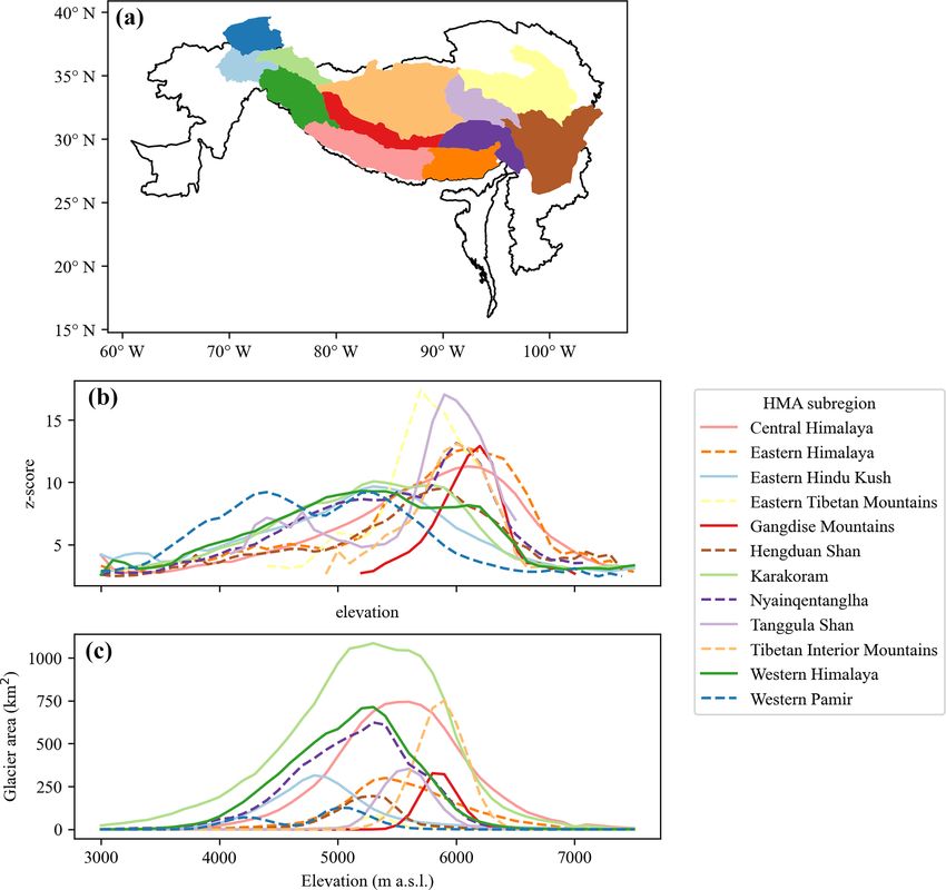
C. Scher et al.: Mapping seasonal glacier melt across the Hindu Kush Himalaya                                                         4469

Figure 1. (a) Hindu Kush Himalaya (HKH) region and 2018 GAMDAM glacierized areas summed across glacio-climate sub-regions from
Shean et al. (2020). An inset map highlights the spatial fidelity of GAMDAM outlines in the top panel. GGI and HKH data overlay a
30 m Shuttle Radar Topography Mission (SRTM) digital elevation model (DEM) hillshade (Farr, 2007). (b) Sentinel-1 ascending- (red) and
descending-swath (blue) footprints acquired across the study region. Ascending-orbit cycle number 56 is highlighted in red to illustrate the
SAR image processing approach for time series analysis across distinct orbit cycles.

as data for comparison with Sentinel-1 backscatter values               ducted across Sentinel-1 A/B ascending- and descending-
(Shea, 2016).                                                           orbit track time series separately and mosaicked into a final
                                                                        image based on a statistical score for seasonal melt magni-
                                                                        tude after classification. To classify snowmelt, we conduct a
3     Methods                                                           pixel-based temporal classification by comparing each image
                                                                        at interval “i” to a dry or frozen winter average backscatter
3.1    Classification                                                   value calculated from January–February for each study year.
                                                                        Due to missing VH acquisitions at some locations during the
We use a threshold-based change detection algorithm applied             2017 frozen months, (January–February), we utilized 2018
to time series radar backscatter intensity to classify melt con-        frozen month reference data for melt retrieval across the cal-
ditions (Ashcraft and Long, 2007). Melt detection is con-               endar year 2017 as regular acquisitions across the HKH be-

https://doi.org/10.5194/tc-15-4465-2021                                                        The Cryosphere, 15, 4465–4482, 2021
Mapping seasonal glacier melt across the Hindu Kush Himalaya with time series synthetic aperture radar (SAR)
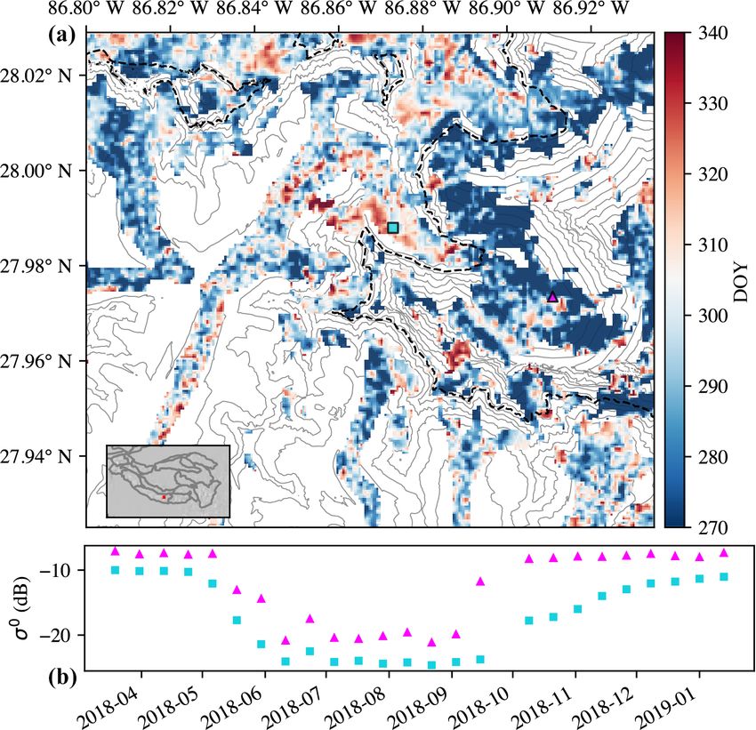
4470                                          C. Scher et al.: Mapping seasonal glacier melt across the Hindu Kush Himalaya

Figure 2. (a) Mean summer (July–August) 2018 cross-polarized (VH) backscatter across an example region in the Trishuli basin, Nepal.
(b) Mean 2018 winter (January–February) VH backscatter from Sentinel-1. (c) Sentinel-2 false-color (near-infrared, green, blue) image
acquired by Sentinel-2 on 30 October 2018. Glacier outlines are shown in blue, and the Yala Glacier base camp meteorological station is
marked in red. Note the snow-covered and bare-ice portions of outlined glaciers and other debris-covered portions of glacier ablation areas.
(d) The difference between mean summer and winter VH backscatter from Sentinel-1.

Table 1. Sentinel-1 image count and orbit paths used in this study.

                           Orbit direction   Number of S-1 images by year                    Relative orbit cycle
                                             2017     2018            2019
                           Descending        4424     5436            5253            4, 5, 19, 20, 33, 34, 48,49,
                                                                               62, 63, 77, 78, 92, 106, 107, 121,
                                                                               122, 135, 136, 150, 151, 164, 165
                           Ascending         5302     6097            6150         12, 13, 26, 27, 41, 42, 55, 56,
                                                                               70, 71, 85, 86, 99, 100, 114, 115,
                                                                               128, 129, 143, 144, 158, 172, 173

gan in late February 2017. Snowmelt at each image acquisi-              have been developed across numerous studies of melt de-
tion interval (mi ) was classified using Eq. (1):                       tection with C-band scatterometer and SAR datasets using
                                                                        both ground-based observations and radar scattering model
          1, if σi0 < σ 0w − b,
       
mi =                                                  (1)               results of changes to backscatter magnitude at the onset of
          0, if σi0 > σ 0w − b,
                                                                        melt. We followed previous studies (Baghdadi et al., 1997;
where the ground-range detected backscatter intensity at                Bhattacharya et al., 2009; Engeset et al., 2002; Nagler and
each image acquisition (σi0 ) within the times series must be           Rott, 2000; Oza et al., 2011; Rott and Mätzler, 1987; Steiner
less than the difference between the mean winter backscat-              and Tedesco, 2014; Trusel et al., 2012) and selected a b
ter (σ 0w ) and a fixed threshold (b). Threshold values (b)             value equal to one-half of the signal power (3 dB). Fig-

The Cryosphere, 15, 4465–4482, 2021                                                          https://doi.org/10.5194/tc-15-4465-2021
Mapping seasonal glacier melt across the Hindu Kush Himalaya with time series synthetic aperture radar (SAR)
C. Scher et al.: Mapping seasonal glacier melt across the Hindu Kush Himalaya                                                         4471

Table 2. Sources of air temperature data used to calculate 3 d average temperature–elevation lapse rates within the central Himalaya for the
2018 calendar year.

        Station name        Date range                 Resolution     Elevation     Latitude   Longitude    Source
                            (dd/mm/yyyy)                               (m a.s.l.)
        Yala Glacier        05/08/2012–                Hourly              4950     28.23252    85.61208    ICIMOD
                            12/31/2018
        Kyanging station    03/22/2012–                Hourly             3,802     28.21081    85.56169    ICIMOD
                            12/31/2019
        Camp II             05/22/2019–                Hourly             6,464      27.9810     86.9023    (Matthews et al., 2019)
                            10/31/2019
        South Col           05/22/2019–                Hourly             7,945      27.9719     86.9295    (Matthews et al., 2019)
                            10/31/2019

ure 3 provides an illustration of the SAR melt signal for a              of pixels employed in regions of overlapping orbital tracks
high-elevation (4950 m a.s.l.) meteorological station, located           based on the sensitivity of the radar backscatter to melting.
at the Yala Glacier base camp. Backscatter values averaged               We apply this metric to choose which orbit direction (ascend-
across the Yala Glacier acquired along the Sentinel-1 A/B                ing or descending) to use for melt classification on a per-pixel
descending-orbit direction are plotted alongside mean daily              basis after applying Eq. (1) across each orbit cycle time series
air temperature recorded at the Yala Glacier base camp auto-             so as to capture the maximum area of melt signals occurring
matic weather station (Shea, 2016). If we consider air tem-              across the complex terrain.
perature above 0 ◦ C to control glacier surface melt at this lo-            Sentinel-1 A/B interferometric wide (IW) swath images
cation, classification accuracy for melt retrieval using Eq. (1)         have a range in viewing angle between 29.1–46.0◦ (ESA).
is 96 % in the VH polarization.                                          Glacier melt retrieval using SAR data commonly begins
                                                                         with a normalization of radar images by viewing angle on a
3.2   Quantifying algorithm performance                                  scene-by-scene basis (Adam et al., 1997; Huang et al., 2011;
                                                                         Rott and Mätzler, 1987; Winsvold et al., 2018). We consider
Sentinel-1 SAR viewing geometry will vary as the local inci-             changes for each individual orthorectified 10 × 10 m pixel
dence angle increases with across-track range. At high inci-             time series across distinct, repeating orbit tracks and direc-
dence angles (far range), the sensitivity to volume scatter is           tions. This approach holds the local incidence angle effec-
diminished, and the melting signal is reduced. At C-band fre-            tively constant for each region observed by a given set of or-
quencies, these effects on volume scatter are strongest only             bit tracks. Glacier melt classification and z-score calculation
at very high incidence angles (closer to grazing) (Nagler and            are carried out across images acquired along identical orbit
Rott, 2000). We classified areas as valid for melt detection us-         tracks in distinct orbit directions (Fig. 1) and mosaicked into
ing a metric of statistical separability for seasonal backscat-          a final dataset for each study year using the greatest z score
ter intensity across frozen and melt periods, which we inter-            observed across each orbit cycle path and in each orbit di-
pret as a measure of the strength of the seasonal melt signal            rection. We thus limit temporal resolution of melt retrievals
Eq. (2):                                                                 to 12 d by choosing only observations from the orbit direc-
      σ 0w − σs0                                                         tion with the greater z score on a per-pixel basis. Time series
z=               ,                                              (2)      analysis of SAR acquisitions on distinct orbit tracks elimi-
       s(σw0 )
                                                                         nates the need to normalize each scene by incidence angle for
where the score for seasonal separability of backscatter in-             the purposes of melt retrieval. This method reduces compu-
tensity (z) was calculated across each SAR pixel’s time                  tational cost and eliminates artifacts that may originate from
series using the difference between the mean winter σ 0w                 overlapping orbit paths and differences in radar viewing an-
(January–February) and summer σ 0s (July–August) season                  gle. Areas where complex topography controls the backscat-
backscatter intensities as compared to the standard deviation            ter should show little time series variability in backscatter
of backscatter across the winter months (σw0 ). In computing             change at the SAR pixel scale when viewed at a distinct and
z, we employed consistent repeat-pass observation geome-                 consistent orbit path and direction and should not pass the
tries, thereby allowing application of the time series melt de-          z-score test.
tection algorithm in regions of complex terrain. This metric                We apply time series melt detection only where inter-
serves as a measure of the magnitude of the seasonal melt                seasonal backscatter intensities are separated by greater than
signal across each pixel’s time series. It is used here as a cri-        2 standard deviations (z > 2), representing better than 98 %
terion to identify valid melt observations and for selection

https://doi.org/10.5194/tc-15-4465-2021                                                        The Cryosphere, 15, 4465–4482, 2021
Mapping seasonal glacier melt across the Hindu Kush Himalaya with time series synthetic aperture radar (SAR)
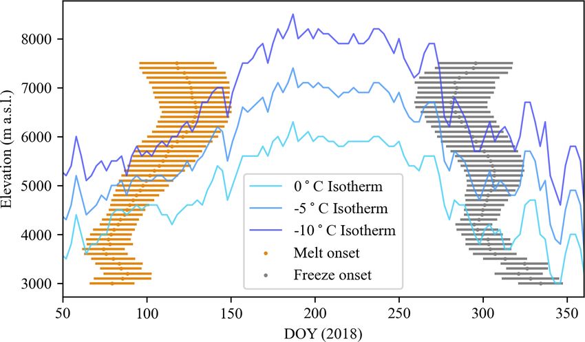
4472                                         C. Scher et al.: Mapping seasonal glacier melt across the Hindu Kush Himalaya

Figure 3. Time series chart of air temperature measured at the Yala Glacier base camp (4950 m a.s.l.) and Sentinel-1 A/B descending
backscatter averaged across the Yala Glacier for the years 2017–2018. Assessment of algorithm performance assuming mean daily air
temperatures above 0 ◦ C indicates active melt results in 96 % accuracy for melt classification across this time series in the VH polarized
backscatter.

confidence in the presence of an annual melt signal. For                3.3   Surface energy balance and surface melting
all locations, the orbit direction and orbit cycle that has the
greatest z value is used for melt classification. We find that          Sentinel-1 SAR (S1-SAR) detects a substantial area and du-
z generally increases with elevation across sub-regions of              ration of melting at elevations where air temperatures should
the HKH and that, across elevation ranges, the mean z is                be well below freezing. Although measurement data in these
above the threshold for melt retrieval, indicating detection            areas are scarce, AWSs installed during 2019 at Mt. Everest,
of a seasonal melt signal across all ranges of glacier eleva-           Nepal, can provide two instances of point-scale validations of
tion spanning the HKH (Fig. 4). Areas of debris cover may               glacier melting using surface energy balance (SEB) model-
exhibit radar brightening with snow-free conditions above               ing based on in situ measurements. As described in Matthews
winter mean (z < 0). These areas occur towards lower ele-               et al. (2020), the highest AWSs on the Earth are installed ad-
vations, where seasonal snow or firn does not have a signif-            jacent to the Khumbu Glacier, Nepal. We use AWS observa-
icant contribution to the seasonal backscatter response, and            tions to compute SEB described in Matthews et al. (2020).
are not included in our melt classification approach follow-            In our SEB modeling, turbulent fluxes are determined us-
ing z-score thresholding. Nonetheless, there exists retriev-            ing the aerodynamic roughness at the glacier surface taken
able melt signals (i.e., z>2) across ablation surfaces such             from measurements in low latitudes (Brock et al., 2006) and
that median window filtering across ablation zones can re-              evaluated over the 5th to 95th percentile of this sample to
sult in a geospatial dataset with more complete coverage. We            capture uncertainty. Surface melting is defined by the glacier
obtain more robust estimates of melting onset and refreeze              surface temperatures (Ts ) that are evolved from air tempera-
by spatially aggregating results of the glacier surface melt            tures and the residual downward glacier heat flux in the iter-
timing (Eq. 1) using a median window filter of 9 × 9 pixels             ative approach from MacDougall et al. (2011). Melting days
after melt classification and z-score validation. Reach-scale           are defined where Ts = 0 ◦ C at any point during the day. The
regions where SAR signals fail the z-score test are thus inter-         Supplement for this paper is provided to describe the SEB
polated over using 9 × 9 pixel median window filtering. The             methodology in further detail (Supplement Sect. S1.1).
complexity of SAR signals involves the diverse scattering                  A comparison of S1-SAR- and SEB-derived melting is
mechanisms on ablation surfaces following the disappear-                shown in Fig. 5. During 2019, the average daily air tem-
ance of seasonal snow. Because sufficient data are retrievable          perature measurements at the Camp II station (Fig. 5a)
on ablation surfaces (i.e., z>2), median window filtering en-           are never above zero but experience above-zero maximum
ables greater spatial continuity in SAR-derived melt retrieval          glacier surface temperatures starting in June 2019 and end-
data. All spatiotemporal characteristics we report herein are           ing in September 2019. At the South Col AWS, the aver-
after median window filtering of melt retrievals from 10 m              age temperature is much less, close to −10 ◦ C on average
native resolution to 90 m resolution. In Fig. 4 we show the             during summer months (Fig. 5b). S1-SAR estimates of sur-
mean z with elevation across HiMAP sub-regions in order                 face melting use two aggregated backscatter time series over
to illustrate the seasonal radar contrast. Mean seasonal melt           90 m × 90 m areas where area centers are located nearest to
magnitude averaged over 100 m elevation bins over all 3 cal-            each of the AWS stations over the Khumbu Glacier, Nepal.
endar years of data shows strong (z>2) melt signals across              For the Camp II AWS, this is centered at 6483 m a.s.l. and
glacio-climatic sub-regions and across all elevation ranges of          for the South Col AWS at 7128 m a.s.l. Melting signals are
significant glaciation.                                                 apparent at both Camp II (Fig. 5c) and South Col (Fig. 5d).
                                                                           Melting is detected at high elevations in both SAR obser-
                                                                        vations and SEB modeling output where daily average air

The Cryosphere, 15, 4465–4482, 2021                                                          https://doi.org/10.5194/tc-15-4465-2021
Mapping seasonal glacier melt across the Hindu Kush Himalaya with time series synthetic aperture radar (SAR)
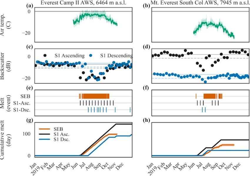
C. Scher et al.: Mapping seasonal glacier melt across the Hindu Kush Himalaya                                                  4473

Figure 4. (a) Glacio-climate sub-regions within the Hindu Kush Himalaya codified in Shean et al. (2020). (b) Mean z score (2017–2019)
by 100 m SRTM elevation bin over each sub-region in the HKH. (c) Mapped glacier area from the GAMDAM database (Sakai, 2019) over
100 m elevation bins derived using the 30 m SRTM DEM (Farr, 2007) for each sub-region.

temperatures remain below zero. We find that S1 and SEB              erage at two locations on the Khumbu Glacier in Nepal and
estimates of surface melting at the Everest Camp II AWS              refreeze to within 16 d. Although limited by observational
(6464 m a.s.l.) have an agreement score – the percentage of          data, the agreement in melt duration between S1-SAR and
days where the SEB and SAR find the same condition – that            SEB modeling, and the understanding of the physical basis
ranges from 73 % to 85 % depending on the parameteriza-              of SAR measurements, we have a high degree of confidence
tion of surface roughness used in SEB estimates of melting.          in our methodology and in the ability of the SAR backscat-
At Mt. Everest South Col (7945 m a.s.l.) the agreement score         ter to detect melting events in data-poor regions such as the
varies from 63 % to 68 %. We find that the S1-SAR finds              HKH.
133 d of melting at Camp II, while the SEB indicates from
93 to 100 d. At Mt. Everest South Col the S1-SAR finds 72 d          3.4   Comparison to temperature–elevation lapse rates
of melting, while the SEB indicates 43 to 56. The start of sur-
face melting at Camp II from SEB modeling is day of year             Melting on glacier surfaces across the HKH is controlled
(DOY) 153 and DOY 142 from S1-SAR; at South Col melt                 by the SEB between the atmosphere and underlaying snow,
onset is DOY 152 from SEB and DOY 146 from S1-SAR.                   firn or ice. We explore the relationship between the S1-SAR-
The end of surface melting at Camp II from SEB modeling              derived surface melting record and air temperature–elevation
is DOY 270 and DOY 290 from S1-SAR. At South Col, re-                lapse rates within the central Himalayas during 2018 us-
freeze at the surface from SEB is DOY 256 and DOY 244                ing data from two meteorological stations within the Lang-
from S1-SAR.                                                         tang valley (Table 1). Temperature–elevation lapse rates were
   Using SEB outputs we find good agreement on surface               determined using 3-day averages of hourly air temperature
melt timings; S1-SAR detects melt onset to within 9 d on av-         measurements interpolated to fill gaps using methods iden-

https://doi.org/10.5194/tc-15-4465-2021                                                    The Cryosphere, 15, 4465–4482, 2021
4474                                          C. Scher et al.: Mapping seasonal glacier melt across the Hindu Kush Himalaya

Figure 5. Air temperature measurements from (a) the Everest Camp II automated weather station (AWS) and (b) the Mt. Everest South
Col AWS are compared to glacier surface melting observations from the Sentinel-1 satellite synthetic aperture radar (SAR). (c) The radar
backscatter from the Khumbu Glacier (at 6483 m a.s.l.) adjacent to the Camp II AWS show a pronounced decrease in backscatter over several
months associated with ongoing surface melting during summer months. Melting is identified when backscatter decreases below a threshold
(dashed line), set at 3 dB below the winter mean (solid line). (d) At the upper reaches of the Khumbu Glacier (7128 m a.s.l.), S1-SAR observes
melting during ascending passes (18:00 local time) but not during descending passes (06:00 local time), except for a brief period during late
June. (f) Timing of surface melt from observation and SEB modeling are compared to S1 ascending and descending observations at (e)
Camp II and (f) South Col AWSs. The cumulative number of melting days from the SEB model and S1-SAR are shown for (g) Camp II and
(h) South Col.

tical for the calculation of temperature–elevation lapse rates           ble 3). Aggregate statistics of melt onset (MO) and freeze
in numerical model studies of snowmelt and glacier wast-                 onset (FO) are calculated across 100 m elevation bins us-
ing in the HKH (Baral et al., 2014). We calculated the dif-              ing the 30 m SRTM (Farr, 2007) digital elevation model for
ference between 3-day average air temperatures and divided               each glacio-climate sub-region as presented in Fig. 4. For all
by the difference in elevation (1148 m) between the two sta-             sub-regions, there is a roughly linear relationship of mean
tions in the Langtang river valley, Nepal. Lapse rates ranged            MO with elevation over most ranges in elevation and a no-
from 5 ◦ C km−1 in July of 2018 to −13.7 ◦ C km−1 in Decem-              ticeable break from elevation lapse rates at high elevations
ber of the same year. Temperature–elevation lapse rates were             distinct to each HiMAP sub-region. The progression of MO
used to extrapolate the maximum elevation of three isotherms             with increasing elevation is consistent with lapse rate temper-
(−10, −5 and 0 ◦ C) for each day of the year in 2018 in or-              ature controls on surface melting for most elevation ranges.
der to compare extrapolated temperatures with melt retrievals            Notably, we find an inflection toward earlier melt onset oc-
from Sentinel-1.                                                         curring at higher elevations (>6000 m a.s.l.). A divergence
                                                                         from lapse-rate-driven melting at high elevations suggests
                                                                         that snowmelt onset may have regional triggers, like strong
4   Results and discussion                                               solar insolation (Matthews et al., 2019) or variable regional
                                                                         weather patterns, such as increases in atmospheric moisture,
A melting signal (z>2) is observed across all regions of sig-            cloudiness and deep convection (Lau et al., 2010).
nificant mapped glacier area contained in the GAMDAM                        In the 3 years of freeze onset (FO) across sub-regions
inventory. Melt retrievals are aggregated across 12 glacio-              we find an elevation dependence as observed in MO, with a
climate sub-regions within the HKH delineated within the                 break in elevation lapse rates beginning around 6000 m a.s.l.
HiMAP dataset (Shean et al., 2020) and averaged across the               (Fig. 6). For much of the HKH, FO occurs during a shorter
calendar years 2017–2019 to report summary statistics (Ta-               period of time than MO. For example, in the central Hi-

The Cryosphere, 15, 4465–4482, 2021                                                            https://doi.org/10.5194/tc-15-4465-2021
C. Scher et al.: Mapping seasonal glacier melt across the Hindu Kush Himalaya                                                                                                                                                                                                                                                                  4475

malaya sub-region, FO has a range of 42 d, while the MO

                                                                   Table 3. Melt retrieval statistics summarized across HiMAP sub-regions and aggregated over 1 km elevation bins from the SRTM 30 m DEM (Farr, 2007). Data for each elevation bin
                                                                   and sub-region are structured, where the first row is the melt onset (MO) in day of year (DOY) and associated MO variance in days, the second row is freeze onset (FO; DOY) and
for this region spans 58 d on average. There is a delay in FO
at elevations above 6000 m a.s.l., relative to elevations below,

                                                                                                                                                                                                                                                     Himalaya

                                                                                                                                                                                                                                                                        317 (6.6)

                                                                                                                                                                                                                                                                                       306 (1.0)

                                                                                                                                                                                                                                                                                                      106 (6.7)
                                                                                                                                                                                                                                                                                                      305 (3.9)

                                                                                                                                                                                                                                                                                                                     123 (2.2)
                                                                                                                                                                                                                                                                                                                     291 (3.0)

                                                                                                                                                                                                                                                                                                                                    111 (4.5)
                                                                                                                                                                                                                                                                                                                                    299 (4.6)
                                                                                                                                                                                                                                                                        75 (5.3)

                                                                                                                                                                                                                                                                                       89 (5.4)
for most glacio-climate sub-regions. (Fig. 6). For example,

                                                                                                                                                                                                                                                     Central

                                                                                                                                                                                                                                                                                       1562

                                                                                                                                                                                                                                                                                                      7668

                                                                                                                                                                                                                                                                                                                     2313

                                                                                                                                                                                                                                                                                                                                    153
in the western Himalaya, FO at 7000 m occurs 26 d later than

                                                                                                                                                                                                                                                                        52
FO at 6000 m a.s.l. and at the same time as 5500 m. (Supple-

                                                                                                                                                                                                                                                     Himalaya

                                                                                                                                                                                                                                                                        317 (7.1)

                                                                                                                                                                                                                                                                                       318 (2.2)

                                                                                                                                                                                                                                                                                                      104 (9.7)
                                                                                                                                                                                                                                                                                                      311 (5.4)

                                                                                                                                                                                                                                                                                                                     127 (4.0)
                                                                                                                                                                                                                                                                                                                     294 (6.8)

                                                                                                                                                                                                                                                                                                                                    111 (3.1)
                                                                                                                                                                                                                                                                                                                                    301 (6.0)
ment Fig. S4). Similarly, in the Karakoram, FO occurs 13 d

                                                                                                                                                                                                                                                                        72 (5.3)

                                                                                                                                                                                                                                                                                       81 (4.8)
                                                                                                                                                                                                                                                     Eastern
later at 7500 m a.s.l. compared to 6500 m a.s.l. In the eastern

                                                                                                                                                                                                                                                                                                      2728
                                                                                                                                                                                                                                                                                       380

                                                                                                                                                                                                                                                                                                                     745
                                                                                                                                                                                                                                                                        26

                                                                                                                                                                                                                                                                                                                                    21
Hindi Kush, FO at 6500 m a.s.l. is delayed by 17 d relative to
FO at 6500 m a.s.l.

                                                                                                                                                                                                                                                     Eastern Hindu
   Signals of delayed refreeze are observed above elevation

                                                                                                                                                                                                                                                                                                      121 (15.5)
                                                                                                                                                                                                                                                                                       108 (4.6)
                                                                                                                                                                                                                                                                                       305 (8.3)

                                                                                                                                                                                                                                                                                                      289 (6.6)

                                                                                                                                                                                                                                                                                                                     135 (5.3)
                                                                                                                                                                                                                                                                                                                     284 (3.1)
ranges that have the greatest z scores across summary statis-

                                                                                                                                                                                                                                                     Kush

                                                                                                                                                                                                                                                                                                      3105

                                                                                                                                                                                                                                                                                                                     167
tics of FO (Supplement Fig. S4). Similarly, MO retrievals

                                                                                                                                                                                                                                                                                       40
                                                                                                                                                                                                                                                                        –
                                                                                                                                                                                                                                                                        –
                                                                                                                                                                                                                                                                        –

                                                                                                                                                                                                                                                                                                                                    –
                                                                                                                                                                                                                                                                                                                                    –
occur earlier in the year in these elevation ranges for most

                                                                                                                                                                                                                                                     Eastern Tibetan
major sub-regions (i.e., western Himalaya, central Himalaya,
the Karakoram) where aggregate FO statistics show delayed

                                                                                                                                                                                                                                                     Mountains

                                                                                                                                                                                                                                                                                                      121 (17.8)
                                                                                                                                                                                                                                                                                       321 (2.9)

                                                                                                                                                                                                                                                                                                      311 (4.8)

                                                                                                                                                                                                                                                                                                                     140 (2.7)
                                                                                                                                                                                                                                                                                                                     297 (1.9)
                                                                                                                                                                                                                                                                                       94 (6.7)
refreeze (Fig. S4). These elevations are above zones of likely

                                                                                                                                                                                                                                                                                                      383
percolation areas, indicated by a large z score, as discussed

                                                                                                                                                                                                                                                                                       25
                                                                                                                                                                                                                                                                        –
                                                                                                                                                                                                                                                                        –
                                                                                                                                                                                                                                                                        –

                                                                                                                                                                                                                                                                                                                     3
                                                                                                                                                                                                                                                                                                                                    –
                                                                                                                                                                                                                                                                                                                                    –
in Sect. 4.1.

                                                                                                                                                                                                                                                     Mountains

                                                                                                                                                                                                                                                                                                                     287 (12.7)
                                                                                                                                                                                                                                                     Gangdise

                                                                                                                                                                                                                                                                                                      107 (3.1)
                                                                                                                                                                                                                                                                                                      298 (6.2)

                                                                                                                                                                                                                                                                                                                     126 (9.2)
4.1   Percolation meltwater hydrology

                                                                                                                                                                                                                                                                                                      1218

                                                                                                                                                                                                                                                                                                                     471
                                                                                                                                                                                                                                                                        –
                                                                                                                                                                                                                                                                        –
                                                                                                                                                                                                                                                                        –
                                                                                                                                                                                                                                                                                       –
                                                                                                                                                                                                                                                                                       –
                                                                                                                                                                                                                                                                                       –

                                                                                                                                                                                                                                                                                                                                    –
                                                                                                                                                                                                                                                                                                                                    –
We observe signals of delayed refreeze on individual glaciers

                                                                                                                                                                                                                                                                                                                                    287 (10.0)
                                                                                                                                                                                                                                                     Hengduan

                                                                                                                                                                                                                                                                        327 (2.6)

                                                                                                                                                                                                                                                                                       323 (2.7)

                                                                                                                                                                                                                                                                                                      112 (7.6)
                                                                                                                                                                                                                                                                                                      318 (2.7)

                                                                                                                                                                                                                                                                                                                     122 (2.7)
                                                                                                                                                                                                                                                                                                                     300 (4.3)

                                                                                                                                                                                                                                                                                                                                    128 (9.5)
                                                                                                                                                                                                                                                                        74 (4.9)

                                                                                                                                                                                                                                                                                       88 (7.1)
indicative of meltwater retention within percolation facies

                                                                                                                                                                                                                                                     Shan

                                                                                                                                                                                                                                                                                                      1351
(Fig. 7). Complete refreeze across the depth of a percolation

                                                                                                                                                                                                                                                                                       263
                                                                                                                                                                                                                                                                        13

                                                                                                                                                                                                                                                                                                                     39
                                                                   associated variance (days), and the third row is the area of melt retrieved in units of square kilometers.

                                                                                                                                                                                                                                                                                                                                    1
zone is delayed relative to percolation zone surfaces because
                                                                                                                                                                                                                                                     Karakoram

liquid water is retained within a percolation zone medium
                                                                                                                                                                                                                                                                        324 (2.3)

                                                                                                                                                                                                                                                                                       101 (5.8)
                                                                                                                                                                                                                                                                                       312 (4.3)

                                                                                                                                                                                                                                                                                                      121 (7.9)
                                                                                                                                                                                                                                                                                                      296 (6.8)

                                                                                                                                                                                                                                                                                                                     123 (7.1)
                                                                                                                                                                                                                                                                                                                     291 (8.6)

                                                                                                                                                                                                                                                                                                                                    116 (5.0)
                                                                                                                                                                                                                                                                                                                                    302 (2.2)
                                                                                                                                                                                                                                                                        84 (3.8)
after the surface has frozen (Paterson, 2016). Completely

                                                                                                                                                                                                                                                                                                      14 208
                                                                                                                                                                                                                                                                                       5433

                                                                                                                                                                                                                                                                                                                     2518
                                                                                                                                                                                                                                                                        843
frozen percolation zones produce some of the largest radar

                                                                                                                                                                                                                                                                                                                                    97
backscatter responses on the terrestrial Earth (Jezek et al.,
                                                                                                                                                                                                                                                     Nyainqentanglha

1994). Because frozen snow and percolation facies are essen-
tially transparent, C-band SAR will be sensitive to the pres-

                                                                                                                                                                                                                                                                                                                                    139 (19.8)
                                                                                                                                                                                                                                                                        324 (3.1)

                                                                                                                                                                                                                                                                                       330 (0.5)

                                                                                                                                                                                                                                                                                                      115 (6.6)
                                                                                                                                                                                                                                                                                                      322 (7.1)

                                                                                                                                                                                                                                                                                                                     126 (3.4)
                                                                                                                                                                                                                                                                                                                     306 (6.7)

                                                                                                                                                                                                                                                                                                                                    292 (8.5)
                                                                                                                                                                                                                                                                        73 (4.5)

                                                                                                                                                                                                                                                                                       90 (7.6)

ence of liquid water across the volume of snowpack or firn
                                                                                                                                                                                                                                                                                       2689

strata (Fischer et al., 2019). Signals of delayed refreeze on                                                                                                                                                                                                                                         5468
                                                                                                                                                                                                                                                                        151

                                                                                                                                                                                                                                                                                                                     284

                                                                                                                                                                                                                                                                                                                                    1
individual glacier are indicative of meltwater storage within
                                                                                                                                                                                                                                                                                                      115 (15.8)
                                                                                                                                                                                                                                                                                                      311 (10.5)

the percolation volume due to meltwater retention. At the
                                                                                                                                                                                                                                                     Tanggula

                                                                                                                                                                                                                                                                                       332 (9.4)

                                                                                                                                                                                                                                                                                                                     150 (1.9)
                                                                                                                                                                                                                                                                                                                     296 (7.6)
                                                                                                                                                                                                                                                                                       94 (6.9)

Khumbu Glacier on Mount Everest, Sentinel-1-retrieved re-
                                                                                                                                                                                                                                                     Shan

                                                                                                                                                                                                                                                                                                      2059
                                                                                                                                                                                                                                                                                       17

                                                                                                                                                                                                                                                                                                                     96
freeze occurs over 30 d later at ∼ 6000 m a.s.l. compared to
                                                                                                                                                                                                                                                                        –
                                                                                                                                                                                                                                                                        –
                                                                                                                                                                                                                                                                        –

                                                                                                                                                                                                                                                                                                                                    –
elevations below 5400 m a.s.l. and above 6200 m a.s.l., indi-                                                                                                                                                                                                                                                                       –
                                                                                                                                                                                                                                                     Tibetan interior

cating that liquid meltwater was retained at elevation ranges
                                                                                                                                                                                                                                                     mountains

                                                                                                                                                                                                                                                                                                      107 (16.0)
                                                                                                                                                                                                                                                                                                      301 (19.3)

between ∼ 5400–6200 m a.s.l. during a month when eleva-
                                                                                                                                                                                                                                                                                                                     133 (4.0)
                                                                                                                                                                                                                                                                                                                     278 (7.7)

tions both above and below this range were recorded as com-
                                                                                                                                                                                                                                                                                                      2916

                                                                                                                                                                                                                                                                                                                     1517

pletely frozen within Sentinel-1-retrieved melt signals. The
                                                                                                                                                                                                                                                                        –
                                                                                                                                                                                                                                                                        –
                                                                                                                                                                                                                                                                        –
                                                                                                                                                                                                                                                                                       –
                                                                                                                                                                                                                                                                                       –
                                                                                                                                                                                                                                                                                       –

                                                                                                                                                                                                                                                                                                                                    –
                                                                                                                                                                                                                                                                                                                                    –

time series of mean Sentinel-1 SAR backscatter for descend-
                                                                                                                                                                                                                                                                                                                     289 (10.8)
                                                                                                                                                                                                                                                     Himalaya

                                                                                                                                                                                                                                                                        322 (3.6)

                                                                                                                                                                                                                                                                                       311 (3.9)

                                                                                                                                                                                                                                                                                                      119 (7.7)
                                                                                                                                                                                                                                                                                                      296 (7.8)

                                                                                                                                                                                                                                                                                                                     119 (9.9)

                                                                                                                                                                                                                                                                                                                                    104 (5.1)
                                                                                                                                                                                                                                                                                                                                    307 (4.9)
                                                                                                                                                                                                                                                     Western

                                                                                                                                                                                                                                                                        78 (9.4)

                                                                                                                                                                                                                                                                                       97 (4.9)

ing orbital nodes from two 250 m buffered points on the
                                                                                                                                                                                                                                                                                       3675

                                                                                                                                                                                                                                                                                                      6279
                                                                                                                                                                                                                                                                        155

                                                                                                                                                                                                                                                                                                                     365

Khumbu Glacier show a rapid increase in SAR backscat-
                                                                                                                                                                                                                                                                                                                                    12

ter magnitude for the higher-elevation location, whereas
                                                                                                                                                                                                                                                                                                                                    123 (10.9)
                                                                                                                                                                                                                                                                                                                                    294 (17.2)

backscatter time series extracted from within the elevation
                                                                                                                                                                                                                                                                        325 (3.8)

                                                                                                                                                                                                                                                                                       114 (6.1)
                                                                                                                                                                                                                                                                                       307 (6.8)

                                                                                                                                                                                                                                                                                                      128 (1.9)
                                                                                                                                                                                                                                                                                                      289 (2.6)

                                                                                                                                                                                                                                                                                                                     119 (3.2)
                                                                                                                                                                                                                                                                                                                     296 (2.9)
                                                                                                                                                                                                                                                     Western

                                                                                                                                                                                                                                                                        90 (7.6)
                                                                                                                                                                                                                                                     Pamir

range of delayed melt offset show a gradual increase in radar
                                                                                                                                                                                                                                                                                       4180

                                                                                                                                                                                                                                                                                                      2820
                                                                                                                                                                                                                                                                        483

                                                                                                                                                                                                                                                                                                                     89

backscatter. We interpret this gradual backscatter increase to
                                                                                                                                                                                                                                                                                                                                    1

be indicative of gradually decreasing liquid water content in
                                                                                                                                                                                                                                                     Elevation Range

the snowpack (or firn) as refreeze progresses from the glacier
                                                                                                                                                                                                                                                                           3000–3999

                                                                                                                                                                                                                                                                                          4000–4999

                                                                                                                                                                                                                                                                                                         5000–5999

                                                                                                                                                                                                                                                                                                                        6000–6999

                                                                                                                                                                                                                                                                                                                                       7000–7999

surface and into the depth of the percolation zone (Fig. 7)
                                                                                                                                                                                                                                                     (m a.s.l.)

(Forster et al., 2014; Miège et al., 2016). This elevation range
(∼ 5400–6200 m a.s.l.) is similar to known elevation ranges

https://doi.org/10.5194/tc-15-4465-2021                                                                                                                                                                                                                                       The Cryosphere, 15, 4465–4482, 2021
4476                                       C. Scher et al.: Mapping seasonal glacier melt across the Hindu Kush Himalaya

Figure 6. Mean melt onset (MO; left) and freeze onset (FO; right) summarized in 100 m elevation bins using the 30 m SRTM digital
elevation model (Farr, 2007) and 12 HiMAP sub-regions (Shean, 2020). The blue-to-red color scale indicates the longitude of the HiMAP
region centroid, where the westernmost regions are shown in dark blue and easternmost shown in dark red.

of percolation zones on the Khumbu Glacier as detailed in re-
cent fieldwork (Matthews et al., 2019, 2020). Similar delays
in refreeze are observed elsewhere across the glacier surface.
SAR backscatter time series showing a gradual increase in
backscatter within regions of known percolation suggest that
there is a relationship between frozen percolation zone depth
and the rate of C-band backscatter change across refreeze
cycles. It has been shown that C-band backscatter gradually
increases with frozen percolation zone depth and decreasing
percolation zone wetness during a refreeze process (Ashcraft
and Long, 2005).

4.2    Spatial variability: radar scattering and glacier
       facies

Imaging radar backscatter intensity and response to surface
melting are linked with glacier facies (Ramage et al., 2000;
Rau et al., 2000; Zhou and Zheng, 2017). Snow melting
on the glacier surface produces a strong decrease in radar
backscatter across all glacier facies. In the accumulation zone
the refreeze signal is also pronounced as the dissipation of
strongly absorbing wet snow at the surface is followed by
volume scattering from deep snowpack and stratified ice              Figure 7. (a) Refreeze timing over the Khumbu Glacier region of
layering. The scattering response to refreeze in the abla-           Mount Everest in the central Himalaya. Red regions of freeze onset
tion zone is more complex and not well characterized. Here,          occur at mid-elevations, indicative of delayed refreeze due to melt-
supraglacier features like crevasses, suncups, debris cover          water retention in percolation zones. The dashed elevation contour
and other heterogeneities are likely to cause highly variable        line is drawn at 6300 m, which was the maximum elevation of a 0 ◦ C
radar scattering mechanisms over short distances upon the            isotherm for the calendar year 2018. (b) Sentinel-1 backscatter time
disappearance of seasonal snow from the ablation surface             series from two points on the Khumbu Glacier, one within known
(Rott and Mätzler, 1987). We use the z-score metric to select        elevations of glacier percolation facies (teal square; 6000 m a.s.l.)
                                                                     and another point at elevations where temperatures likely do not
areas where radar backscatter increases substantially during
                                                                     exceed 0 ◦ C annually (pink triangle; 6600 m a.s.l.).
the refreeze process. However, since scattering response dur-
ing the transition from wet snow will differ with various sur-
face features (e.g., bare ice, debris and supraglacier ponding),

The Cryosphere, 15, 4465–4482, 2021                                                       https://doi.org/10.5194/tc-15-4465-2021
C. Scher et al.: Mapping seasonal glacier melt across the Hindu Kush Himalaya                                                     4477

Figure 8. Melt retrievals averaged over the calendar years 2017–2019 in the central Himalaya and Karakoram regions. (a) Mean melt onset
(DOY) in the central Himalaya. (b) Mean melt onset (DOY) over the Siachen Glacier in the Karakoram region. (c) Mean freeze onset (DOY)
in the central Himalaya. (d) Mean freeze onset (DOY) over the Siachen Glacier in the Karakoram region. Data overlay a 30 m Shuttle Radar
Topography Mission (SRTM) DEM hillshade (Farr, 2007).

it is difficult to isolate the refreeze response. Average z is        gation. In ablation areas with lower sensitivity to melting, we
minimum in the HKH across the lowest-elevation glacier sur-           hypothesize that snow-off conditions result in brightening of
faces (3000–4000 m a.s.l.), whereas z is maximum at unique            the radar signal due to surface scattering contributions from
elevation ranges within sub-regions (Figs. 4, S4). Ablation           wet debris, bare ice or other ablation surface heterogeneities.
zone surfaces (at lower elevations) do not exhibit the magni-         For this reason, at lower elevations where annual air temper-
tude of backscatter intensity of percolation zones and there-         atures exceed 0 ◦ C (i.e., where temperature–elevation lapse
fore show lesser seasonal contrast in backscatter compared            rates hold), lapse rate estimates of elevation might be more
to higher elevations. These differences are also apparent in          robust estimates of FO using this approach. Overall, surface
the spatial granularity of melt retrievals from the S1-SAR            melting signals appear to be consistent with expectations of
product, as shown in Fig. 8. Ablation zone surfaces on val-           temperature lapse rates (i.e., earlier melting and later refreeze
ley glaciers show spatial heterogeneity in MO indicative of           at lower elevations) across elevations where annual air tem-
supraglacial features, like debris cover rather than randomly         peratures likely exceed 0 ◦ C (
4478                                         C. Scher et al.: Mapping seasonal glacier melt across the Hindu Kush Himalaya

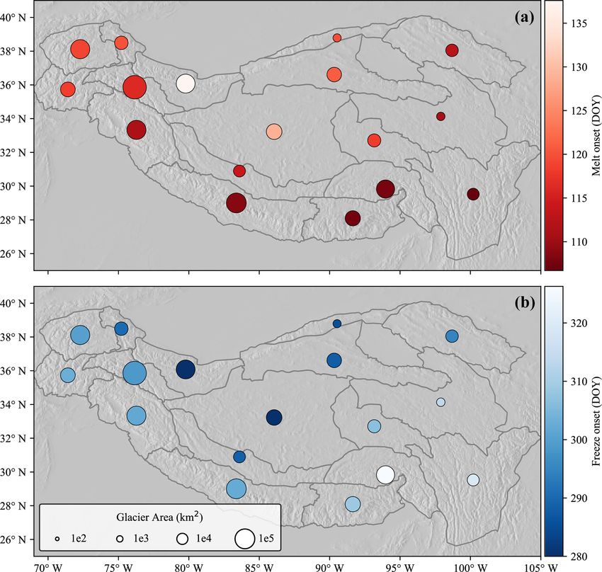
Figure 9. Melt onset (a) and freeze onset (b) averaged over 2017–2019 plotted over an SRTM 30 m DEM hillshade (Farr, 2007). Melt
retrievals are averaged across HiMAP glacio-climate sub-regions (Bolch et al., 2019a; Shean et al., 2020) and scaled by the mapped glacier
area within each sub-region.

addition to average melt onset and offset by sub-region in             across glaciers between 5000–7500 m a.s.l. MO and FO sig-
Fig. 9.                                                                nals are retrieved on days and at elevations where lapse-rate-
                                                                       derived temperatures do not exceed −10 ◦ C, which strength-
4.3    Considerations of temperature–elevation lapse                   ens and expands recent in situ observations on glacier melt
       rates                                                           at the Khumbu Glacier in the Mount Everest region showing
                                                                       that incident shortwave radiation drives melt at these temper-
We compare SAR retrievals of MO and FO to temperature–                 atures and elevations (Matthews et al., 2019). Here we ob-
elevation lapse rates derived within a catchment in the central        serve that, even at these extreme elevations (>7000 m a.s.l.),
Himalaya to investigate SAR retrievals alongside lapse rate            melt signals persist for over 4 months across the central
assumptions of glacier melt status using methods and AWS               Himalaya, which suggests that liquid water is retained at
data for the construction of lapse rates from prior studies in         these high elevations across a seasonal melt cycle and may
the Langtang valley, central Himalaya (Baral et al., 2014).            not be hydrologically negligible. In radar-derived observa-
In 2018, we observe that the average MO is found to follow             tions there is a discrepancy between SAR and lapse-rate-
the range in isotherms for elevations ∼ 3600 to 6500 m a.s.l.          estimated melting records that occurs at elevations extending
(Fig. 10). Below and above these elevations and for FO, we             1 km above the maximum 0 ◦ C isotherms in the central Hi-
find episodic melting events occurring over a range of ele-            malaya. Glaciated areas in the central Himalaya at elevations
vations. This is especially apparent in the FO around day of           greater than 6300 m a.s.l. – the approximate maximum ele-
year 280, where FO occurs within a roughly 1-month period

The Cryosphere, 15, 4465–4482, 2021                                                         https://doi.org/10.5194/tc-15-4465-2021
C. Scher et al.: Mapping seasonal glacier melt across the Hindu Kush Himalaya                                                    4479

                                                                      tion may be useful for interrogating meteo-climatic drivers of
                                                                      heterogeneity in glacier wasting dynamics across the HKH.

                                                                      5   Conclusions

                                                                      Synthetic aperture radar time series backscatter images and
                                                                      glacier extent maps derived from optical imagery have long
                                                                      been proposed to inform hydrologic and glaciologic research
                                                                      across the global cryosphere; however a harmonized dataset
                                                                      of glacier surface melt does not exist. We retrieve glacier sur-
                                                                      face melt timing and duration for the study years 2017–2019
                                                                      across the HKH region using time series C-band SAR from
Figure 10. Sentinel-1 SAR-retrieved melt onset (orange) and freeze
onset (gray), with spatial variability at ± 1 standard deviation,     the Sentinel-1 A/B satellites and an inventory of 105 432
across the central Himalaya region. The elevations of the 0, −5       glaciers spanning 83 102 km2 of ice-covered area. We quan-
and −10 ◦ C isotherms from 2018 are overlaid for comparison. Melt     tify the magnitude of the seasonal melt signal by comparing
signals are recorded in excess of 3 months at elevations extending    mean summer and winter backscatter using a z-score met-
>1 km above the maximum elevation of the 0 ◦ C isotherm, indica-      ric and retrieve constraints on seasonal melt characteristics
tive of a sustained presence of liquid water within the snow matrix   across all glaciated elevations of HKH at 90 m spatial and
across these high-elevation ranges.                                   12 d temporal resolution. Melt conditions in surface energy
                                                                      balance models of glacier melt, driven by in situ meteoro-
                                                                      logical data from Mount Everest, fall within the date ranges
vation of the 0 ◦ C isotherm for 2018 – account for 21.58 %           of melt retrievals recorded in Sentinel-1 SAR data. Compar-
(2,453 km2 ) of total glaciated area within the region.               ison of melt retrievals to temperature–elevation lapse rates
                                                                      calculated using two high-elevation meteorological stations
                                                                      in the central Himalaya reveals that melt onset persists for
4.4   Melt retrievals and glacio-climate sub-regions
                                                                      over 4 months at elevations where extrapolated air tempera-
                                                                      ture fields do not exceed −10 ◦ C. Melt is retrieved across all
The 3-year record of Sentinel-1 SAR retrievals of glacier             elevation ranges of HKH glaciers, which suggests that a dry-
melt status represents a baseline measurement for the HKH             snow accumulation zone in the HKH region does not exist.
region. The summary melt statistics are aggregated over               Meltwater retention is indicated within known glacier perco-
HiMAP sub-regions in order to compare melt retrievals                 lation zones on Mount Everest through signals of delayed re-
and sub-regional estimates of glacier mass loss (Shean et             freeze. Delayed refreeze occurs across the HKH at elevations
al., 2020). Overall, the HKH sub-regions with the most                with the greatest seasonal contrast in backscatter intensity, at-
rapid mass loss between 2000–2010 tabulated in Shean et               tributable to radar scattering in percolation facies. Melt sig-
al. (2020) (eastern Himalaya, Hengduan Shan, Nyainqêntan-             nals persist for a greater portion of the year in regions known
glha) exhibit the greatest number of melt days on average             for rapid contemporary glacier wasting (i.e., central and east-
in 2017–2019 from Sentinel-1 retrievals. Sub-regions with             ern Himalaya sub-regions), whereas regions with a more sta-
slower mass loss show less melt duration relative to regions          ble glacier mass balance (i.e., western Himalaya, Karako-
with accelerated mass loss. For example, over the 2017–2019           ram) exhibit a shorter duration of annual melt. We produce a
period the Karakoram has an average surface melt duration             geospatial data product of melt onset (DOY) and freeze onset
16 d shorter than the eastern Himalaya. Although Sentinel-1           (DOY) spanning glaciers of the HKH region at 90 m spatial
retrievals of glacier melt status for 3 calendar years do not         resolution for the calendar years 2017–2019 and plan to re-
make up a climatic record, we observe that between 2017–              lease annual updates to this dataset each calendar year across
2019 there was on average less duration of melting in regions         the mission duration of Sentinel-1. The methods presented in
where in situ data and climate models indicate that frozen            this study can provide the basis for an operational monitoring
winter precipitation contributes to glacier accumulation de-          system of glacier surface melt dynamics and aid the develop-
spite warming global climate (Karakoram, Hindu Kush, east-            ment and assessment of surface energy balance models of
ern Pamir, western Himalaya) (Kääb et al., 2015; Kapnick              glacier ablation across the global cryosphere.
et al., 2014; Palazzi et al., 2013). We interpret shorter du-
ration of annual melt days in the western regions of the
HKH as a potential indicator of the “Karakoram anomaly”               Code and data availability. The   data    are     available
reflected in the Sentinel-1 data record. Because the meteo-           from the National Snow and Ice Data Center here:
climatic drivers of the Karakoram anomaly are still under de-         https://doi.org/10.5067/05I6ZHZWHSVV   (Steiner   et    al.,
bate (Farinotti et al., 2020), Sentinel-1 retrievals of melt dura-    2021). The code used to produce the data is available here:

https://doi.org/10.5194/tc-15-4465-2021                                                     The Cryosphere, 15, 4465–4482, 2021
You can also read