Machine learning approach to muon spectroscopy analysis
←
→
Page content transcription
If your browser does not render page correctly, please read the page content below
Journal of Physics: Condensed Matter

PAPER • OPEN ACCESS

Machine learning approach to muon spectroscopy analysis
To cite this article: T Tula et al 2021 J. Phys.: Condens. Matter 33 194002

View the article online for updates and enhancements.

                              This content was downloaded from IP address 86.131.88.181 on 18/06/2021 at 15:42
Journal of Physics: Condensed Matter

J. Phys.: Condens. Matter 33 (2021) 194002 (11pp)                                                                        https://doi.org/10.1088/1361-648X/abe39e

Machine learning approach to muon
spectroscopy analysis
T Tula1 , G Möller1 , J Quintanilla1,∗ , S R Giblin2 , A D Hillier3 ,
E E McCabe1 , S Ramos1 , D S Barker1,4 and S Gibson1
1
  School of Physical Sciences, University of Kent, Park Wood Rd, Canterbury CT2 7NH, United Kingdom
2
  School of Physics and Astronomy, Cardiff University, Cardiff CF24 3AA, United Kingdom
3
  ISIS Facility, STFC Rutherford Appleton Laboratory, Chilton, Didcot Oxon, OX11 0QX, United
Kingdom
4
  School of Physics and Astronomy, University of Leeds, Leeds, LS2 9JT, United Kingdom

E-mail: J.Quintanilla@kent.ac.uk

Received 20 November 2020, revised 21 December 2020
Accepted for publication 5 February 2021
Published 26 April 2021

Abstract
In recent years, artificial intelligence techniques have proved to be very successful when
applied to problems in physical sciences. Here we apply an unsupervised machine learning
(ML) algorithm called principal component analysis (PCA) as a tool to analyse the data from
muon spectroscopy experiments. Specifically, we apply the ML technique to detect phase
transitions in various materials. The measured quantity in muon spectroscopy is an asymmetry
function, which may hold information about the distribution of the intrinsic magnetic field in
combination with the dynamics of the sample. Sharp changes of shape of asymmetry
functions—measured at different temperatures—might indicate a phase transition. Existing
methods of processing the muon spectroscopy data are based on regression analysis, but
choosing the right fitting function requires knowledge about the underlying physics of the
probed material. Conversely, PCA focuses on small differences in the asymmetry curves and
works without any prior assumptions about the studied samples. We discovered that the PCA
method works well in detecting phase transitions in muon spectroscopy experiments and can
serve as an alternative to current analysis, especially if the physics of the studied material are
not entirely known. Additionally, we found out that our ML technique seems to work best with
large numbers of measurements, regardless of whether the algorithm takes data only for a
single material or whether the analysis is performed simultaneously for many materials with
different physical properties.
Keywords: machine learning, muon spectroscopy, muon spin relaxation experiment, principal
component analysis, identifying phase transitions, time-reversal symmetry breaking
superconductors
(Some figures may appear in colour only in the online journal)

1. Introduction                                                                      condensed matter physics, ML is well suited for many tasks
                                                                                     ranging from predicting materials properties based on exist-
Machine learning (ML) methods are now widely used in many                            ing databases and pattern recognition in specific experimen-
areas of physics, usually as a tool to analyse large amounts of                      tal data to analysing theoretical models of quantum materials.
data [1–3]. These techniques are particularly useful in regres-                      Prominent examples include the prediction of novel materials
sion, classification and dimensionality reduction tasks which                        [4–6], identification of phase transitions in models of magnetic
are often required in processing scientific data. Specifically in                    materials starting from Ising models [7–12], reaching com-
                                                                                     plex spin liquids in Heisenberg systems [13] and the detection
∗
    Author to whom any correspondence should be addressed.                           of entanglement transitions from simulated neutron scattering

1361-648X/21/194002+11$33.00                                                     1      © 2021 The Author(s). Published by IOP Publishing Ltd    Printed in the UK

                 This is an open access article distributed under the terms of the Creative Commons Attribution 4.0 License.
                 Any further distribution of this work must maintain attribution to the author(s) and the title of the work, journal citation and DOI.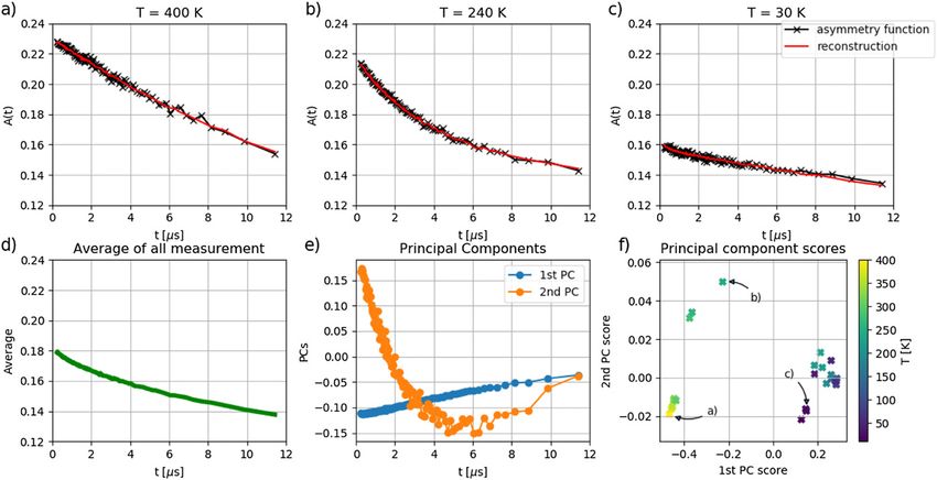
J. Phys.: Condens. Matter 33 (2021) 194002                                                                                        T Tula et al

data [14]. ML algorithms were also proven to be state of the            magnetic field of the sample will affect the final distribution of
art techniques in simulations of wave functions [15] or den-            positron detection events.
sity matrices [16–19] for many-body quantum systems and                    A commonly used setup is to have symmetrical detectors
the tomographic reconstruction of many-body wave functions              in front of (F) and behind (B) the sample (with respect to the
from experimental data [20].                                            muon beam). The quantity that we are interested in is the differ-
    Much of the research in this area so far is concerned with          ence in number of counting events between the two detectors
simulation or analysing simulated data, however it has also             as a function of time N i (t), i ∈ {F, B}, called the asymmetry
been shown that such techniques can detect phase transitions            function
from piezoelectric relaxation measurements [21] or discover-                                          NB (t) − NF (t)
ing existence of translational symmetry-breaking states from                                 A(t) =                   .                (1)
                                                                                                      NB (t) + NF (t)
real, electronic quantum matter images [22]. Here we want to
apply a simple dimensionality reduction algorithm to real data          The analysis of the data involves fitting specific asymme-
from muon spin rotation (μSR) experiments [23] to see if we             try curves to the experimentally-obtained curve. Given some
can detect phase transitions for a range of different materials.        knowledge of the underlying physics for a particular material
We decided to use the data from this type of experiment since           and/or some justified assumptions, a model can be formulated,
models used in μSR data analysis require previous understand-           and the asymmetry curve can be derived from it. In some sim-
ing of the local environment of muons inside probed sample,             ple cases appropriate closed-form expressions can be derived
which is not always easily available. Therefore, as an alterna-         [28, 29], though more generally ad hoc calculations are nec-
tive, we propose the use of linear principal component analysis         essary [30]. For some systems, our understanding is still not
(PCA), a simple unsupervised ML technique which does not                sufficiently developed for such predictions—for instance, the
make any prior assumption, yet is known to reveal correlations          theory of zero-field muon spin relaxation (ZF-μSR) in super-
within the data. By demonstrating that this approach works, we          conductors with broken time-reversal symmetry (TRS) is still
propose that it may serve as a more unbiased way of detecting           in its infancy [31].
phase transitions observed in μSR experiments. In this paper                In practice, for complex systems it is customary to
we apply PCA to μSR data from a small number of supercon-               use a phenomenological expression featuring several
ducting and magnetic materials whose physics are known to               adjustable parameters. Electronic order can then manifest as a
differ widely from each other. In particular we explore the tech-       temperature-dependence of those parameters. For instance, in
nique for data from time reversal symmetry breaking (TRSB)              ZF-μSR investigations of superconductors [32] one often fits:
superconductors, which are among the most difficult to anal-
                                                                                  Aphen. (t) = A0 GKT (σ, t) exp(−λt) + Abckg ,          (2)
yse, since changes in experimental data are very subtle. Other
materials that we have tested are a symmetry breaking antifer-          where GKT (σ, t) is the Kubo–Toyabe function describing cou-
romagnet (BaFe2 Se2 O) and a spin liquid (LuCuGaO4 ). We find           pling to static, randomly-oriented magnetic moments [28, 29,
some evidence that PCA can detect important features such as            33, 34] with relaxation rate λ and Gaussian magnetic field
phase transitions. We also find that when the system is trained         strength distribution with standard deviation σ. The param-
on all the materials, taken together, the results improve—even          eters σ, λ, A0 , Abckg are then interpreted to describe distinct
though the materials chosen have different underlying physics.          relaxation mechanisms. In conventional superconductors these
    The paper is organised as follows. In section 2, we briefly         parameters tend to evolve smoothly through the superconduct-
present the set up of the muon spectroscopy experiment and              ing critical temperature, T c . In other systems, marked changes
the current method of analysing the data from it. In section 3,         in some of these parameters occur at T c [35]. These are often
we present the principal component (PC) analysis in general             interpreted as evidence of broken TRS and in some systems
and how we used it in practice. Then, in section 4, we move             this has been confirmed by Kerr effect or SQUID magnetom-
on to results of applying PCA to data from different materials          etry. Quite frequently, it is found that only one of the fitting
and discuss in detail how the method performs. We summarise             parameters in equation (2) depends on temperature. This is
the results in section 5.                                               usually either σ or λ, which naturally leads to a classification
                                                                        of TRS-breaking superconductors. We note, however, that the
2. Muon spectroscopy experiment                                         relaxation rates involved are very small, meaning that only a
                                                                        small portion of the curve described by equation (2) is repre-
The general setup of a μSR experiment design to measure the             sented in the experimental data sets (due to the finite lifetime
local magnetic environment consists of spin-polarised muons             of the muon). As a result, this classification may not always
being implanted into a sample, which is surrounded by multi-            be as robust as would be desirable. For instance, some super-
ple positron detectors. Once they enter the sample, muons will          conductors that are expected to have very similar underlying
interact with the atoms causing them (muons) to thermalise              physics can fall in different classes. Such is the case of the
and eventually implant themselves at some sites of the system.          proposed nonunitary triplet superconductors LaNiC2 [36] and
The spin of the muons will start to precess due to the local mag-       LaNiGa2 [37], whose asymmetry functions are best described
netic field and the muons will eventually decay into positrons          by a temperature-dependent σ and λ, respectively, in spite of
and neutrinos with a mean life time of 2.2 μs. The positron             experimental [38, 39] and theoretical [32] evidence of very
velocity direction is directly connected to the muon spin ori-          similar underlying physical mechanisms. Likewise, the muon
entation at the time of decay [24–27] and therefore the intrinsic       spin relaxation rate in spin glasses can often be described by

                                                                    2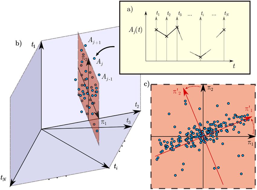
J. Phys.: Condens. Matter 33 (2021) 194002                                                                                                               T Tula et al

Figure 1. Representation of the PC analysis in high-dimensional data space. The asymmetry functions A j (t) consist of N real values
representing time windows ti , i = 1, 2, . . . , N. Each of ti can be thought of as independent dimension (a). In this framework, we can
represent each individual asymmetry function A j as a point in N-dimensional space (b)5 . We expect correlations between different
asymmetry functions, which means that the data can be projected into a smaller subspace of initial N-dimensional space, without loss of
information. The actual PC analysis (c) can be represented as a rotation of initial coordinate space (π 1 , π 2 ) into a new (π 1 , π 2 ) so that most
of the covariance is captured by the π 1 dimension. The vectors in new basis (π 1 , π 2 ) are called PCs and are usually numbered according to
the amount of covariance they hold. Note: the projection onto π 1 × π 2 plane is not a part of PC analysis. The PCA rotates whole data space
(after removing the average so that the cluster of data is centred at the beginning of coordinates) and then one can choose how many PCs
(dimensions) must be used to represent the data well, based on the total covariance they hold.

a stretched exponential function (with temperature-dependent                   material at different temperatures, we expect correlations
exponent), reflecting the variation in local spin fluctuation                  between those points. PCA can detect these correlations by
rates as well as non-exponential decay at muon sites [40–42].                  first removing the average of all experimental curves, then
However, fitting experimental data can give parameter values                   measuring the covariance for each dimension and linearly
that are not expected from standard models/numerical analysis                  transforming the coordinates so that the new basis of the data
[43]. In conclusion, it would be highly desirable to have a way                space consists of only few directions that capture most of the
of analysing the temperature-dependence of μSR spectra that                    covariance. The vectors of this new basis are called PCs and
can detect electronic ordering transitions without the need to                 can be thought of as the most common deviations from the
assume any a priori fitting functions.                                         average curve. We can reconstruct all of the measurements
                                                                               used in the analysis by adding to the average a linear combina-
                                                                               tion of PCs. We can also represent each curve by specifying its
3. PC analysis                                                                 projections onto the PCs, which are often called PC ‘scores’.
                                                                               Thus, PCA provides us with a more compact description of the
To analyse the data from a muon spectroscopy experiment                        experimental data and additionally we can recover information
without making assumptions about the physical nature of the                    about linear correlations from their magnitudes (or PC scores)
materials, we decided to use an unsupervised ML technique                      and shapes (the PCs, or PC vectors).
called PCA [7, 44, 45]. The concept behind it—in the con-                          In the example shown in figure 1(c), most of the data lies
text of muon spectroscopy experiment and asymmetry func-                       in two-dimensional space π 1 × π 2 . PCA finds new orthogo-
tions—is presented in figure 1. We can think about differ-                     nal directions (π 1 , π 2 ), because there exist linear correlation
ent experimental measurements as points in some data space
with N dimensions. In the case of muon spectroscopy, each
                                                                               5 In panel (b), each of the directions t
dimension i = 1, 2, . . . , N represents a time window ti , within                                                 1 , t2 , . . . , t N should be understood as being
                                                                               orthogonal to any other, thus spanning an N-dimensional target space repre-
which the positron detections are measured. If the measure-                    senting a full dataset from an individual measured asymmetry function as a
ments are not random but correspond, for example, to the same                  function of time.

                                                                           3
J. Phys.: Condens. Matter 33 (2021) 194002 T Tula et al
between the π 1 and π 2 coordinates of data points. We can the method will not perform well. Fortunately, looking at the
now specify each asymmetry curve by its projection onto π 1 , eigenvalues of S, one can decide if the linear PCA is sufficient,
whereas before we would have to state both π 1 and π 2 coor- based on the decrease of PC scores which is often illustrated
dinates. We do lose some information about the individual in a so-called scree plot of the PC scores against their index.
data points in this way, but we gain in the more compact In order to account for the experimental noise in the data,
representation of asymmetry curves. Usually, more than one we have re-binned raw data into new time windows according
PC is needed to represent the data well. The number of impor- to the measurement error. Since the error increases with time,
tant PCs varies with different data sets and can be decided by wider time windows are required at larger times to get com-
looking at how much covariance each PC holds. parable errors. Hence, available measurement points are more
We now present a more specific description of the PCA widely spaced at later times, as can be seen in figures 2(a)–(c).
method. Each measurement can be represented as a vector It is important to re-bin all of the measurements simultane-
T
a j = A j(t1 ), A j(t2 ), . . . , A j(tN ) ,6 with its values equal to the ously because all time-windows t1 , t2 , . . . , tN in our matrix A
values of asymmetry function at specific times and the index have to be the same for all columns for the PCA to be well
j = 1, 2, . . . , M taken to label the distinct measured asymme- defined. Note that this specification mirrors the treatment in
try curves that we want to analyse by the algorithm. We fur- regression methods, where less weight is attributed to data at
ther assume that all measurements were recorded for the same long times to account for the larger measurement errors. Our
set of N measurement times ti , taken relative to the time for binning procedure is discussed in detail in appendix A.
implanting the muon into the material. We combine the vectors
a j in column form to construct a matrix A
3.1. Philosophy of our PCA approach
⎡ ⎤
A1 (t1 ) A2 (t1 ) . . . AM (t1 ) It is worth noting that in the PCA method presented above
⎢ A1 (t2 ) A2 (t2 ) . . . AM (t2 ) ⎥
⎢ ⎥ we do not have to make any assumptions about the shapes of
A=⎢ . . . . ⎥ (3)
⎣ . . .
.
. . . ⎦
. asymmetry curves. There are no hyperparameters to vary, and
A1 (tN ) A2 (tN ) . . . AM (tN ). SVD gives a unique representation of the sought asymmetry
functions (up to a simultaneous change of sign of the PCs and
In the next step we remove the mean of each vector dimension the associated scores). Therefore we think that it provides an
(i.e., averaging over the column index) so that the whole data interesting alternative to fitting methods, where some initial
is centred around the coordinate origin, as shown in figure 1. knowledge of the probed material is needed. We would like to
We end up with a matrix X with elements given by emphasize that it does not necessarily yield better results, but
M it can be applied to any type of input data reflecting all possible
1 shapes of asymmetry functions. Furthermore, by examining
[X]i j = A j(ti ) − Ak (ti ). (4)
M k =1 scree plots of the PC scores, we are always able to judge how
well the method performs in compressing the relevant data.
The most common way for obtaining PCs is to perform a sin- In figure 2, we show an example that illustrates how the
gular value decomposition of X. To this end, we evaluate the method detects changes in the shape of a set of experimentally
covariance matrix measured asymmetry functions, obtained for a single material
1 at different temperatures. The way in which those functions
S= XXT , (5)
M−1 differ from each other is reflected in their respective scores
for the 1st and 2nd PCs. Both high temperature (a) and low
such that the eigenvectors of S are the PCs and the correspond- temperature (c) measurements have almost linear shape and
ing eigenvalues indicate the amount of covariance captured by they only differ in the values for the first PC score. Looking
the given PC. If we write the eigenvectors into a matrix U, then at the 1st PC shape (panel (e), blue curve), we can see that it
a table of scores C for each measurement can be obtained by is also almost linear and when multiplied by a large negative
the matrix product value—as it is for high temperature asymmetry function—and
C = UT X, (6) then added to the average (d), it increases the overall slope.
and the full reconstruction of the initial experimental data is For the low temperature curve, it is added with positive sign,
expressed as which means that it will instead decrease the slope. We can
R = UCT . (7) see that it is exactly the difference between two asymmetry
functions (a) and (c). On the other hand the middle curve (b)
The previously discussed usefulness of the method derives
differs mostly in second PC scores from the other two. When
from the fact that we can choose only the few PCs that capture
the second PC vector ((e), orange curve) is multiplied by a pos-
most of the covariance in order to accurately reconstruct the
itive value and added to the average, it creates a more convex
initial data. Naturally, a large reduction in the number of rel-
curve, which is reflected by the shape of the corresponding
evant PCs does not have to arise for all possible data sets, as
asymmetry function (b).
singular value decomposition only performs a linear transfor-
As a final remark on applying PCA to muon spec-
mation—in particular, if the data has non-linear correlations
troscopy data, we state that the method presented here cannot
distinguish between sources of differences between asymme-
6 Here A(t) stands for the measured quantity as defined in equation (1). try functions. This means that it might be affected by physical
4J. Phys.: Condens. Matter 33 (2021) 194002 T Tula et al
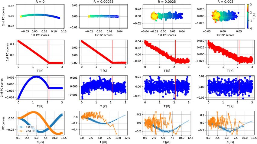
Figure 2. An illustration of how PC analysis can be used to reduce the dimensionality of a muon data set. The set consists of a sizeable
number of experimentally-obtained muon asymmetry functions A(t). The black curves in panels (a)–(c) present three particular examples.
Each curve has 110 time stamps and therefore constitutes a point in a 110-dimensional space. PCA yields a small number of PCs which,
through linear combination, can accurately describe any curve in the data set. In our case, we find the two PCs shown in panel (e). The
reconstruction of the original data using the PCs and the average (d) (see equation (4)) can be obtained by the formula
reconstruction = average + 1st PC score × 1st PC + 2nd PC score × 2nd PC. From that we can interpret the PCs as the most common
deviations from the average curve. The reconstructions are shown, for our three examples, by the red curves in panels (a)–(c). This gives an
accurate reconstruction and therefore enables us to represent each curve by a single point on a two-dimensional plane (f). For this example
we used 25 A(t) curves for the material BaFe2 Se2 O obtained at 25 different temperatures.
phenomena which are intrinsic to muons and not the probed zero and with a standard deviation7 Σsim (t) depending on time
material, such as thermal or quantum hopping of the muons. after muon implantation as:
These effects have been studied in copper [46–48] and bat-
tery materials [49–52], and mostly affect the tail of asym- Σsim (t) = R(at + b). (9)
metry curves. More investigation is required to see if PCA is Errors observed in real measurements increase with time t
able to filter out those effects by capturing them in a single due to the overall smaller number of events detected at later
PC. times. The parameters A0 , σ(T ), Λ, Abckg , R, b, and a were
chosen to match experimental data of one of the TRSB super-
4. Results and discussion conductors we studied (LaNiGa2 ). In addition to the parame-
ters reflecting experimental conditions, we studied the effect
4.1. PCA for simulated data of different error amplitudes R (which in experiments would
correspond to experiments undertaken with different amounts
To illustrate characteristic results of performing PCA on of time allocated for integrating the signal) in order to verify
asymmetry functions, we first consider an example applica- robustness of the PCA approach. Our results from the appli-
tion to synthetic data generated from model Kubo–Toyabe cation of PCA to these simulated data is displayed in figure 3.
functions GKT (σ, t) with added error E(t). Each such simu- We have included four possible cases of ‘noise’ amplitudes
lated asymmetry function was taken from the general form ranging between no error and twice the error we expect from
given by our measurements. The PCA on clean data clearly captures the
transition temperature T c assumed in the simulated data, which
Asim (t; T) = A0 GKT (σ(T), t) exp(−Λt) + Abckg + E(t), (8) separates regions of temperature with or without variation of
the PC scores with T. The first principal score dependency
is found to be very robust to added noise, even for the cases
where we have further encoded a dependency of σ(T ) associ-
where the error is much larger than expected experimentally.
ated with a symmetry-breaking phase transition in many super-
conductors with TRSB, such that σ(T ) ∼ constant for T > T c ,
while varying linearly below T c . The error values were gener- 7
We use the symbol Σ for the standard deviation of simulated errors, to
ated from a Gaussian distribution N(μ = 0, Σsim ) centred on distinguish it from the parameter σ of the Kubo–Toyabe form.
5J. Phys.: Condens. Matter 33 (2021) 194002 T Tula et al
Figure 3. Results of PCA performed on Kubo–Toyabe functions for a range of different simulated error. The third column (R = 0.0025)
corresponds to error similar to our experimental measurements. On top row are the values of 1st vs 2nd PC scores and the change with
temperature, 2nd and 3rd row are showing how PC scores change with temperature (the vertical red line corresponds to expected phase
transition) and on bottom row the shapes of two most important PC are shown. The scaled curve of first PC without error was presented on
the background of cases with noise.
By contrast, the second PC does not seem to hold any useful magnetic susceptibility data collected on several samples sug-
information for realistic noise level. Note also the small overall gest a magnetic phase transition at ∼115 K [54, 55] which
scale of the second PC score. Nevertheless, the phase transi- is now thought to be due to Fe3 O4 -related impurities and is
tion is always clearly visible in the 1st PC, which motivates not intrinsic to the main phase [54]; (c) there’s no evidence
using PCA for experimental data. for the low-temperature ∼40 K phase transition from neutron
powder diffraction [54] or heat capacity data [56] and this
4.2. PCA for experimental data phase transition is thought to involve freezing of spin fluctua-
We applied PC analysis to data from zero-field μSR exper- tions. It is striking that this unsupervised ML analysis correctly
iments for a range of different materials. Among them identified the two phase transitions intrinsic to BaFe2 Se2 O
are TRS breaking superconductors8 (LaNiGa2 , LaNiC2 , without the need for complementary data. We think that this
LaNi1−x Cux C2 ), spin liquid (LuCuGaO4 ) and an antiferro- reflects the strength of both the PCA analysis and the μSR
magnet (iron oxyselenide BaFe2 Se2 O). We first performed technique.
the analysis for each material separately. The shape of the The changes in the asymmetry function are more subtle
two most important PCs and the dependence of the scores on for the superconducting materials (second-fifth column on
temperature are presented on figure 4. figure 4), but the behaviours of PC scores still change at the
Our technique worked best for the antiferromagnetic mate- critical points. We stress that in conventional superconductors
rial (first column on figure 4), for which both expected we would not expect any change of zero-field muon-spin relax-
phase transitions are clearly visible. Although the magnetic ation at the superconducting transition temperature T c . By con-
behaviour of the antiferromagnet BaFe2 Se2 O is relatively sim- trast, LaNiC2 and LaNiGa2 are known to exhibit such changes,
ple [54], this understanding has been challenging to arrive at: and this is believed to be a manifestation of their internally-
(a) T N ∼ 240 K is clear from neutron powder diffraction exper- antisymmetric, non-unitary triplet (INT) pairing states with
iments but is more subtle in magnetic susceptibility measure- TRSB [32]. In the case of LaNiC2 (third column), we only
ments [54–56] due to the layered nature of the material; (b) have one point above the phase transition and therefore we do
not expect visible change. That is confirmed in PC score plots.
8 TRSB in LaNiGa and LaNiC is well established [32]. To our knowledge, Worth mentioning is also the LaNi0.9 Cu0.1 C2 case, in which
2 2
evidence for TRSB in the closely-related case of LaNi1−x Cux C2 is presented there seem to be more than one critical point, at least in the
here for the first time. behaviour of the 1st PC score. That might be caused by some
6J. Phys.: Condens. Matter 33 (2021) 194002 T Tula et al
Figure 4. Results of PC analysis performed independently for each material. The top row presents the shapes of the 1st and 2nd PCs. For
almost all the cases second principal does not look as smooth as the 1st PC. The second and third row display the dependence of PC scores
on temperature for the 1st and 2nd PCs, respectively. The red vertical lines indicate approximately where we expect phase transitions to
occur [53, 54]. The last row presents a scree plot for the amount of covariance that each PCs captures. Here, blue lines indicate how many
PCs are needed to capture 80% of the total covariance.
Figure 5. Results of PC analysis performed simultaneously on experimental data from all materials. The first and second row display the
dependence of PC scores on temperature for the 1st and 2nd PCs, respectively. The red vertical line indicate approximately where we expect
phase transitions to occur [53, 54].
other phase transition but more probably it is caused by limita- available for these types of materials, since most ML algo-
tions of the method. One solution to that problem would be to rithms perform better the more data is provided. It is important
look also at the 2nd PC score, where only one transition point to note that we can still resolve the changes in the scores of 1st
is prominent. Overall, linear PCA seems to be performing bet- and 2nd PCs, at least for LaNiGa2 and LaNi0.9 Cu0.1 C2 .
ter for the spin liquid and antiferromagnetic materials than for The last studied material is a proposed spin liq-
the TRS breaking superconductors analysed in this paper, as is uid—LuCuGaO4 . Muons have been used as a proof of a
evidenced in our scree plots (the last row on figure 4). For the spin liquid state, as it can be argued that the resultant dynam-
first four materials, even the last few PCs hold a significant ics could show a plateau in the relaxation rate with reducing
amount of covariance9. That may imply that the data has non- temperature where no long range order is detected [57]. In
linear correlations or that we did not have not enough data our case the PCA shows no evidence for a phase transition,
even though a plateau is observed, likely indicating there is
9 The singular value decomposition yields min(N, M) singular values, so for no phase transition as the proposed liquid state is entered.
the case of N > M the covariance captured by the last PC will formally vanish, Because the most significant PCs for the TRS breaking
by definition. superconductors look similar for all the cases studied, in hope
7J. Phys.: Condens. Matter 33 (2021) 194002 T Tula et al
Figure 6. Comparison of PCA method, when performed on different amounts of data. The rows correspond to results of PCA when applied
to data from single material (first row), from two materials (second row), from three materials (third row), from four materials (fourth row)
and all materials (fifth row). The materials used are named to the left of the plots. The first four columns present the shapes of PCs and the
last column shows scree plots, with blue vertical lines indicating number of PCs that are needed to capture 80% of covariance. The
improvement of the method can be seen in PC curves, which gradually become smoother functions.
of improving results for TRSB systems, we proceed to apply In particular, the evolution of PC scores as a function of tun-
PCA to all of the experimental data simultaneously. The results ing parameters provides insights into the location of possible
for PC scores are presented on figure 5 and the improvement phase transitions. Comparing this analysis to a more conven-
of PCs are shown on figure 6. The PCs are now much smoother tional approach, based on regression analysis using standard
functions and additionally, only three PCs are sufficient to cap- fitting functions, we find that PCA is typically at least as sen-
ture 80% of the observed covariance. The scores of the first sitive, if not more. More importantly, the PCA approach is
PC did not change much for all materials, despite their differ- free from any underlying assumptions about the physics of the
ent physical properties. This is probably connected to the fact observed material: rather than assuming a specific form of a
that all data come from the same type of experiment and all fitting function (e.g. Kubo–Toyabe or stretched exponential),
asymmetry functions are similar in general. PCA discovers the PCs that describe a given system, without
We note that the data for both LaNi1−x Cux C2 materials human intervention. This is the salient feature of the method
was previously unpublished. Using PCA, we were able to we put forward and it means that the same, universal analysis
see signs of the superconducting phase transition in zero- can be applied to any material.
field muSR experiments, which is the first evidence that the In addition to the universality of our method, we have found
TRSB of LaNiC22 also exists in these Cu-doped materials.
that the quality of the results is enhanced when data for mul-
The increased onset temperature is consistent with the known
tiple materials are analysed as a joint dataset, even when the
enhancement of T c with Cu doping [53].
underlying physics of each system being considered are quite
different. The ability to thus enhance understanding gained
5. Conclusions from a new experiment based on existing data goes beyond
the possibilities of preexisting approaches, where data for each
We have proposed the use of PC analysis to process muon spin material is necessarily analysed and fitted in isolation, and
spectroscopy data, and in particular to aid with the identifi- overarching commonalities are anticipated in advance by the
cation of features relating to phase transitions in the probed formulation of a suitable fitting function. We anticipate this
materials. Our results demonstrate that the representation of could offer great advantage when deployed in large-throughput
the observed asymmetry functions in the space of PC vectors user facilities. In particular, given the advantages gained from
is sensitive to changes in the physics of the observed system. combining multiple data sets, our results suggest a new way
8J. Phys.: Condens. Matter 33 (2021) 194002 T Tula et al
to leverage recently-developed open-data tools and policies reference [54]. JQ acknowledges support from the EPSRC
[58, 59]. under the project ‘Unconventional superconductors: new
We hope that our unsupervised ML approach to muon spec- paradigms for new materials’ (Grant No. EP/P00749X/1). GM
troscopy data analysis could become one of the standard tools gratefully acknowledges support by the Royal Society under
used in that field. In addition to its virtue, noted above, of pro- University Research Fellowship URF\R\180004.
viding a unified way of treating all muons data, we believe
our approach can also accelerate future experiments, as the
Data availability statement
treatment within this framework will require less data to be col-
lected before signatures of the physics can emerge—especially
The data that support the findings of this study are available
if data from previous experiments is used to enhance the
upon reasonable request from the authors.
analysis of new materials as outlined above. In addition, the
simplicity of the analysis means that it could easily be per-
formed immediately while experimental measurements are Appendix A. Re-binning of data
being taken, thus opening the possibility to inform the conduct
of the experiment in real time. At the other end of the spectrum, The error in muon spectroscopy measurements increases at
it is also possible to conduct experiments where much larger later times due to the smaller number of overall positron detec-
data sets are gathered [60]. Our simulations suggest that our tion events. Since PCA treats each dimension (time window)
method applied to such data might yield valuable new insights equally, one needs to pre-process the raw data by re-binning
into phase transitions. They also would be ideal additions to the time windows. While this differes from the exact way
such past-experiment data bank. Given the advantages gained in which errors are treated in a standard fitting procedure,
from combining multiple data sets, our results should encour- where a weight function is applied to give less weight to data
age the community to gather historic and future measurements with larger errors, our approach is broadly equivalent in that
in a common database in order to harvest the benefits of this it makes sure that the standard errors of the rebinned time
approach. points are roughly the same for every measurement. Specif-
A possible future extension of our work would be to deploy ically, we have set up an algorithm for re-binning the data,
an additional unsupervised ML technique to analyse the output such that each new time bin holds the same magnitude of
of our analyses as presented here. The principal score depen- error averaged over all measurements. To illustrate how the
dencies (as shown in figure 5) in the method presented here still algorithm proceeds, let us consider the matrix E, holding
need to be processed by human eye to establish phase transi- the raw values of standard deviations at each time point and
tion temperatures. There exist ML tools that could categorise for each asymmetry curve (similarly to the matrix A from
different phases from the PC scores, that have been shown to equation (3)):
work well with model data [61]. It would be interesting to ⎡ ⎤
apply them to our problem. E1 (t1raw ) E2 (t1raw ) . . . EM (t1raw )
⎢E1 (t2raw ) E2 (t2raw ) . . . EM (t2raw )⎥
⎢ ⎥
E=⎢ . .. .. .. ⎥, (A.1)
Individual author contributions ⎣ .. . . . ⎦
E1 (tNraw ) E2 (tNraw ) . . . EM (tNraw )
T Tula implemented the PCA algorithm and performed the
analysis of the simulated and experimental data presented where M is the number of asymmetry functions that we con-
in this paper under supervision from J T Quintanilla and G sider in the analysis and N corresponds to the number of time
Möller. S R Giblin, A D Hillier, E E McCabe and S Ramos windows in raw data. We set the first time window t1 to be
provided, formatted and commented on the experimental data. equal to t1raw , which holds the average error of
D S Barker performed a preliminary study of PCA applied
M
to experimental and simulated μSR data under supervision 1
Ēt1 = Ei (t1raw ). (A.2)
of J Quintanilla, with further input from S Gibson. T Tula M i =1
wrote the manuscript in close consultation with G Möller and
J Quintanilla and with input from all co-authors. Then we iterate over traw to create new bins in the following
j
way: suppose we created a new bin tk−1 by including raw data
up to the original bin at time traw
j−1 . We then evaluate
Acknowledgments
Ēt1
We would like to thank Stephen Blundell, Tom Lancaster and , (A.3)
Roberto De Renzi for helpful discussions about the content of Ētraw
j
the paper.
TT is supported by the EPSRC via a DTA studentship with Ētraw
j
= M1 M raw
i=1 Ei (t j ). We know that (A.3) is smaller
under Grant No. EP/R513246/1 and by the School of Phys- than 1, since the standard deviation is increasing with time due
ical Sciences, University of Kent. SR and EEM are grate- to decreasing muon counts. If (A.3) is close to one, then the
ful to Mr Ben Coles (for BaFe2 Se2 O synthesis) and to Dr amount of averaged error is similar to the first bin and we can
Fiona Coomer (experimental support) for the μSR data from leave the time window tk = traw j . However, if it reaches certain
9J. Phys.: Condens. Matter 33 (2021) 194002 T Tula et al
threshold, we add another time window traw
j+1 and evaluate:
[12] Hu W, Singh R R P and Scalettar R T 2017 Phys. Rev. E 95
062122
Ēt1 [13] Greitemann J, Liu K, Jaubert L D C, Yan H, Shannon N and
. (A.4) Pollet L 2019 Phys. Rev. B 100 467
(Ē traw
j
)2 + (Ētraw
j+1
)2 [14] Twyman R, Gibson S J, Molony J and Quintanilla J 2020 Prin-
cipal component analysis of diffuse magnetic scattering: a
We repeat this procedure until theoretical study arXiv:2011.08234
[15] Carleo G and Troyer M 2017 Science 355 602–6
Ēt1 [16] Nagy A and Savona V 2019 Phys. Rev. Lett. 122
≈ 1, (A.5) 250501
Lk −1
raw )2
(Ēt j+l [17] Vicentini F, Biella A, Regnault N and Ciuti C 2019 Phys. Rev.
l =0 Lett. 122 250503
[18] Hartmann M J and Carleo G 2019 Phys. Rev. Lett. 122
L −1 250502
and we set a new time bin tk = L1k l=k 0 traw
j+l .
[19] Yoshioka N and Hamazaki R 2019 Phys. Rev. B 99 214306
When the different asymmetry functions come from the
[20] Torlai G, Mazzola G, Carrasquilla J, Troyer M, Melko R and
same material, we expect our method of re-binning to work Carleo G 2018 Nat. Phys. 14 447–50
well. One might expect that problems could arise if we con- [21] Li L, Yang Y, Zhang D, Ye Z-G, Jesse S, Kalinin S V and
sider sets of measurements for different materials of strongly Vasudevan R K 2018 Sci. Adv. 4 eaap8672
different amount of statistics. However, one can prove that as [22] Zhang Y and et al 2019 Nature 570 484–90
[23] Blundell S J 1999 Muon-spin rotation: a brief introduction
long as the time dependency of the error follows the same func-
http://users.ox.ac.uk/~sjb/musr/musr.html (online; accessed
tional behaviour for those sets (i.e., the errors differ just in a 11 Sep 2020)
scale factor), the re-binning will not be affected. Generically, [24] Schenck A G E 1985 Muon Spin Rotation Spectroscopy Prin-
we expect that the overall envelope of the number of counts is ciples and Applications in Solid State Physics (Boca Raton,
set by the exponential decay of muons, which is set by the uni- FL: CRC Press)
[25] Cox S F J 1987 J. Phys. C: Solid State Phys. 20 3187
versal muon lifetime, and material-specific details will provide
[26] Blundell S J 1999 Contemp. Phys. 40 175–92
sub-dominant changes to this overarching behaviour. [27] Lee S L, Cywinski R and Kilcoyne S H (ed) 1999 Muon Science:
Muons in Physics, Chemistry and Materials (Boca Raton, FL:
Appendix B. Software CRC Press)
[28] Kadono R, Imazato J, Matsuzaki T, Nishiyama K, Nagamine K,
Yamazaki T, Richter D and Welter J-M 1989 Phys. Rev. B 39
We wrote implementation of PCA for data from experiment as 23–41
a package for python. Current version of the code, finished at [29] Uemura Y J 1999 Muon Science: Muons in Physics, Chemistry
the time of publishing this article, can be found in [62]. and Materials (Boca Raton, FL: CRC Press)
[30] Onuorah I J, Bonfà P and De Renzi R 2018 Phys. Rev. B 97
174414
ORCID iDs [31] Atsushi T, Susumu Y and Kazumasa M 2015 J. Phys. Soc. Japan
84 094712
[32] Ghosh S K, Smidman M, Shang T, Annett J F, Hillier A, Quin-
T Tula https://orcid.org/0000-0001-9820-4615
tanilla J and Yuan H 2020 J. Phys.: Condens. Matter 33
G Möller https://orcid.org/0000-0001-8986-0899 033001
J Quintanilla https://orcid.org/0000-0002-8572-730X [33] Hayano R S, Uemura Y J, Imazato J, Nishida N, Yamazaki T
and Kubo R 1979 Phys. Rev. B 20 850–9
[34] Kubo R 1981 Hyperfine Interact. 8 731–8
References [35] Ghosh S K, Csire G, Whittlesea P, Annett J F, Gradhand
M, Újfalussy B and Quintanilla J 2020 Phys. Rev. B 101
[1] Zdeborová L 2017 Nat. Phys. 16 602 100506(R)
[2] Carleo G, Cirac I, Cranmer K, Daudet L, Schuld M, Tishby N, [36] Hillier A D, Quintanilla J and Cywinski R 2009 Phys. Rev. Lett.
Vogt-Maranto L and Zdeborová L 2019 Rev. Mod. Phys. 91 102 117007
2773 [37] Hillier A D, Quintanilla J, Mazidian B, Annett J F and Cywinski
[3] Mehta P, Bukov M, Wang C-H, Day A G R, Richardson R 2012 Phys. Rev. Lett. 109 097001
C, Fisher C K and Schwab D J 2019 Phys. Rep. 810 [38] Chen J, Jiao L, Zhang J L, Chen Y, Yang L, Nicklas M, Steglich
1–124 F and Yuan H Q 2013 New J. Phys. 15 053005
[4] Sumpter B G, Vasudevan R, Potok T and Kalinin S V 2015 npj [39] Weng Z F et al 2016 Phys. Rev. Lett. 117 027001
Comput. Mater. 1 15008 [40] Nuccio L, Schulz L and Drew A J 2014 J. Phys. D: Appl. Phys.
[5] Xue D, Balachandran P V, Hogden J, Theiler J, Xue D and 47 473001
Lookman T 2016 Nat. Commun. 7 11241 [41] Campbell I A, Amato A, Gygax F N, Herlach D, Schenck A,
[6] Conduit B D, Jones N G, Stone H J and Conduit G J 2017 Mater. Cywinski R and Kilcoyne S H 1994 Phys. Rev. Lett. 72
Des. 131 358–65 1291–4
[7] Wang L 2016 Phys. Rev. B 94 195105 [42] Keren A, Mendels P, Campbell I A and Lord J 1996 Phys. Rev.
[8] Carrasquilla J and Melko R G 2017 Nat. Phys. 13 431–4 Lett. 77 1386–9
[9] van Nieuwenburg E P L, Liu Y-H and Huber S D 2017 Nat. Phys. [43] Yadav P et al 2019 Phys. Rev. B 99 214421
13 435–9 [44] Géron A 2019 Hands-on Machine Learning with Scikit-Learn,
[10] Wetzel S J 2017 Phys. Rev. E 96 022140 Keras, and TensorFlow: Concepts, Tools, and Techniques
[11] Broecker P, Carrasquilla J, Melko R G and Trebst S 2017 Sci. to Build Intelligent Systems (Sebastopol, CA: O’Reilly
Rep. 7 8823 Media)
10J. Phys.: Condens. Matter 33 (2021) 194002 T Tula et al
[45] Jolliffe I T and Cadima J 2016 Phil. Trans. R. Soc. A 374 [54] Coles B D, Hillier A D, Coomer F C, Bristowe N C, Ramos S
20150202 and McCabe E E 2019 Phys. Rev. B 100 024427
[46] Luke G M, Brewer J H, Kreitzman S R, Noakes D R, Celio M, [55] Lei H, Ryu H, Ivanovski V, Warren J B, Frenkel A I,
Kadono R and Ansaldo E J 1991 Phys. Rev. B 43 3284–97 Cekic B, Yin W G and Petrovic C 2012 Phys. Rev. B 86
[47] Kadono R, Imazato J, Matsuzaki T, Nishiyama K, Nagamine K, 195133
Yamazaki T, Richter D and Welter J-M 1989 Phys. Rev. B 39 [56] Han F, Wan X and Shen Band Wen H H 2012 Phys. Rev. B 86
23–41 014411
[48] Kadono R, Imazato J, Nishiyama K, Nagamine K, Yamazaki T, [57] Khuntia P et al 2016 Phys. Rev. Lett. 116 107203
Richter D and Welter J M 1984 Hyperfine Interact. 17 109–15 [58] ISIS Neutron and Muon Source data repository 2020 https://isis.
[49] McClelland I, Johnston B, Baker P J, Amores M, Cussen E J and stfc.ac.uk/Pages/ICAT.aspx (online; accessed 7 Oct 2020)
Corr S A 2020 Annu. Rev. Mater. Res. 50 371 [59] PANDATA initiative 2020 http://pan-data.eu (online; accessed
[50] Amores M, Baker P J, Cussen E J and Corr S A 2018 Chem. 7 Oct 2020)
Commun. 54 10040–3 [60] Wilkinson J M and Blundell S J 2020 Phys. Rev. Lett. 125
[51] Amores M, Ashton T E, Baker P J, Cussen E J and Corr S A 087201
2016 J. Mater. Chem. A 4 1729–36 [61] Van Nieuwenburg E P L, Liu Y-H and Huber S D 2017 Nat.
[52] Sugiyama J, Mukai K, Ikedo Y, Nozaki H, Månsson M and Phys. 13 435–9
Watanabe I 2009 Phys. Rev. Lett. 103 147601 [62] Tula T, Möller G, Quintanilla J, Barker D S and Gibson
[53] Sung H H, Chou S Y, Syu K J and Lee W H 2008 J. Phys.: S 2021 TymoteuszTula/PCA_Exp: PCA_Exp_v0.1 https://
Condens. Matter 20 165207 zenodo.org/badge/latestdoi/313070471
11You can also read