Kinematics reconstruction of the EAS-like events registered by the TUS detector

accepted for publication in JHEP

 Kinematics reconstruction of the EAS-like events
 registered by the TUS detector

 Sergei Sharakin, Oliver Isac Ruiz Hernandez, 
arXiv:2107.01359v1 [astro-ph.IM] 3 Jul 2021

 Lomonosov Moscow State University, Skobeltsyn Institute of Nuclear Physics,
 GSP-1, Leninskie Gory, Moscow, 119991, Russia
 Benemérita Universidad Autónoma de Puebla, Facultad de Ciencias Físico Matemáticas,

 Avenida San Claudio y 18 Sur, C.P. 72570, Puebla, México

 E-mail: sharakin@mail.ru

 Abstract: The Tracking Ultraviolet Set-up (TUS) is the world’s first orbital imaging detector of
 Ultra High Energy Cosmic Rays (UHECR) and it operated in 2016-2017 as part of the scientific
 equipment of the Lomonosov satellite. The TUS was developed and manufactured as a prototype
 of the larger project K-EUSO with the main purpose of testing the efficiency of the method for
 measuring the ultraviolet signal of extensive air shower (EAS) in the Earth’s night atmosphere.
 Despite the low spatial resolution (∼ 5×5 km2 at sea level), several events were recorded which
 are very similar to EAS as for the signal profile and kinematics. Reconstruction of the parameters of
 such events is complicated by a short track length, an asymmetry of the image, and an uncertainty
 in the sensitivity distribution of the TUS channels. An advanced method was developed for the
 determination of event kinematic parameters including its arrival direction.
 In the present article, this method is applied for the analysis of 6 EAS-like events recorded
 by the TUS detector. All events have an out of space arrival direction with zenith angles less
 than 40◦ . Remarkably they were found to be over the land rather close to United States airports,
 which indicates a possible anthropogenic nature of the phenomenon. Detailed analysis revealed a
 correlation of the reconstructed tracks with direction to airport runways and Very High Frequency
 (VHF) omnidirectional range stations.
 The method developed here for reliable reconstruction of kinematic parameters of the track-like
 events, registered in low spatial resolution, will be useful in future space missions, such as K-EUSO.

 Keywords: ultra-high-energy cosmic rays, reconstruction, cosmic ray detectors, TUS, orbital
 detector, Lomonosov satellite

Contents

1 The TUS detector and events with tracks 1
 1.1 EAS-like TUS events 2
 1.2 Arrival direction 4

2 LTA reconstruction scheme 6
 2.1 LTA and its hyperparameters 6
 2.2 Simulated events reconstruction 7
 2.3 Event-by-event reconstruction 8

3 TUS events reconstruction 10

4 Discussion 13

5 Conclusions 17

1 The TUS detector and events with tracks

The TUS detector is a very sensitive telescope looking into the nadir direction from space, aimed
at measuring extensive air showers (EAS) produced by ultra-high-energy cosmic rays in the at-
mosphere. This is the first attempt to perform the EAS measurement technique, proposed by
John Linsley [1]. The detector was launched on board the Lomonosov satellite on 28.04.2016
from Vostochny cosmodrome (Russian Federation) to the polar sun-synchronous orbit with height
 = 470 − 500 km and inclination 97.3◦ . The telescope consists of two main parts: the mirror-
concentrator and the photodetector in its focal plane. The photodetector has 256 channels (“pixels”)
disposed as a square matrix of 16 modules by 16 channels (pixel map). Each channel is rep-
resented by a photomultiplier tube (PMT) Hamamatsu R1463 with a square window (15 mm ×
15 mm). An UV filter is placed in front of each PMT to limit the wavelength range of measurements
(300-400 nm).
 The effective focal distance of the mirror is = 1.5 m, so the angular resolution of one pixel
is equal to 10 mrad, which corresponds to ∼ 5 km on the ground. The total field of view (FOV) of
the detector is 9◦ × 9◦ or about 80 × 80 km2 .
 The temporal resolution of the detector in the fastest mode of operation (EAS mode) is
determined by a gate time unit, GTU = 0.8 s. Each recorded event is a set of 256 digital signals
represented by ADC counts (waveforms), with a duration of 256 GTUs (≈ 205 s). More details
about the detector and first results of measurements can be found in [2, 3].
 The detector operated till late 2017 and registered almost 80,000 events in the EAS mode.
Several preliminary EAS candidates have been selected in the TUS data earlier [4, 5]. The
Lomonosov–UHECR/TLE Collaboration continues the TUS data analysis. One of the main tasks

 –1–

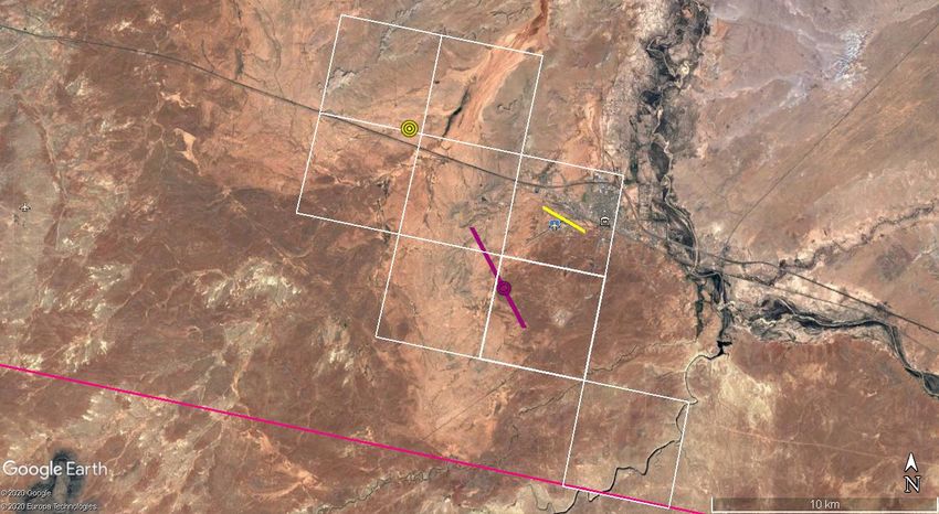
of this analysis is to search for and study events in which the signals are similar to that expected
from an EAS. In total, about 100 events with the typical signal profile shape and duration for an
EAS have been selected to date. However, only a few of them exhibit the EAS-like kinematics.

1.1 EAS-like TUS events
When analyzing the events measured by the TUS detector, several classes with common properties
were identified, see for example, [3]. Some of the most mysterious events are the so-called EAS-like
events, with a spatio-temporal pattern typical for the EAS fluorescence.
 For these events, it is possible to identify a large number of hit pixels (channels whose signal
significantly exceeds the background) that line up on the pixel map along some direction (“thick”
track). The total signal of the hit pixels with a subtracted background (the light curve) has a
characteristic fast increase with its subsequent slightly slower decline. The full duration of the
signal is about 0.1 ms.
 Six of the events registered by the TUS detector have these properties, see table 1. Interestingly,
all events were recorded over the United States and over land.
 In [6], one of these events, TUS1610031, was reconstructed to test the hypothesis of its EAS
origin. However, an energy of this EAS candidate estimated by the amplitude of the luminescence
is at least 1 ZeV according to simulation in the ESAF (EUSO Simulation and Analysis Framework)
software, [7]. Due to small total exposure (1200-1400 km2 sr year) and a very steep spectrum of
cosmic rays in this energy range, a chance the TUS to have registered such an extremely energetic
cosmic particle is very low (order of 10−3 − 10−5 ). Some other possible explanations of the origin
of this event were suggested, including anthropogenic sources.

Table 1. List of EAS-like events and their location (geographical coordinates correspond to the center of the
TUS FOV). The number of hit pixels is indicated in the last column.

 Event Time (UTC) Latitude Longitude Location # hit pixels
 TUS161003 05:48:59 44.08◦ N 92.71◦ W Minnesota (USA) 10
 TUS161031 10:25:18 61.30◦ N 155.69◦ W Alaska (USA) 8
 TUS170915 06:30:18 40.31◦ N 107.07◦ W Colorado (USA) 12
 TUS171010 04:26:04 34.83◦ N 77.39◦ W North Carolina (USA) 15
 TUS171029a 06:39:09 35.27◦ N 110.78◦ W Arizona (USA) 8
 TUS171029b 11:13:26 65.90◦ N 168.07◦ W Alaska (USA) 9

 In this paper, we summarize information about the EAS-like events by reconstructing their
kinematics. In addition to the features of the light curve and the image on the photodetector, these
events are characterized by a noticeable time shifts of the signal peaks in the hit channels – the
motion of the image along the track. Figure 1 shows the active signals of the TUS170915 (and their
smooth approximations). Here we grouped 12 selected pixels (see insert in figure 2) into 4 “lines” -
directions perpendicular to the photodetector modules. The peak of the signals summed along the
lines moves sequentially in time from the line ch = 16 to the line ch = 13. Such movement is typical
 1Hereinafter TUS events are identified by indicating the registration date, so the first event in table 1 was triggered on
October 03, 2016. To distinguish the last two events recorded on the same day, suffixes a and b are used.

 –2–

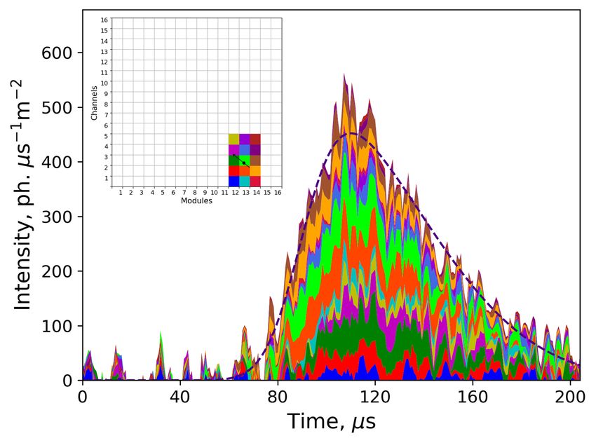
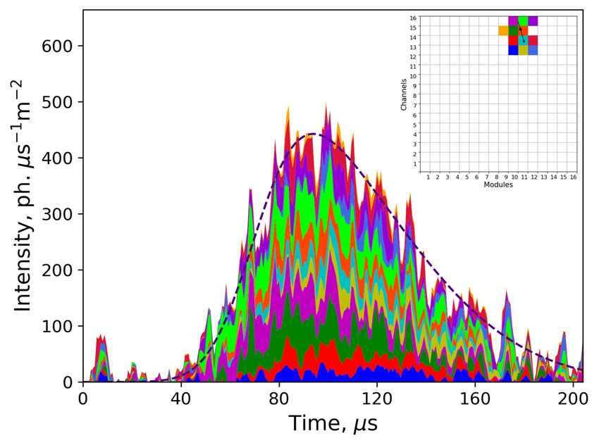
Figure 1. Peak movement for TUS170915 from line ch=16 (blue curve) to ch=13 (magenta). Dashed lines
are results of the SkewGauss approximation.

for a relativistic object with a luminescence region of the size of one channel or less on the FOV
(“point-like” source).
 Hit pixels selection for each of these events was carried out by the amplitude of the moving
average of the signal MA(8) (with a time window equals 8 GTUs). The value of the amplitude of the
smoothed signal over its stationary value was studied at different thresholds, then the pre-selected
channels were tested by location in space (neighboring pixels) and time (proximity to maximum).
The number of hit pixels is indicated in the last column of the table 1.
 At the next stage of the analysis, the active signal extraction was made for each of the selected
channels. To do this, the ADC counts was initially converted into the photon flux density at the
entrance pupil of the detector, expressed as the number of photons per square meter per microsecond
(for more details of this procedure, see [6]). After that, the signal was approximated by a parametric
function with an asymmetric shape of the waveform. The SkewGauss function (the density function
of the Skew-Normal distribution [8]) was chosen for this, and an additional constant was added to
evaluate a background (Base Level of the signal).
 Active signal extraction allows us to reconstruct the light curve of the event. To quantify
the latter, the sum of the all active signals was approximated by the SkewGauss function again.
For example, figure 2 shows the result of such a parameterization over 12 selected channels of
the TUS170915. The signal value at the maximum (amplitude of the light curve) was m =
442 ph/( s m2 ), which is approximately two times more than that of the event TUS161003. In
this paper, we will characterize the luminescence duration by the full duration at half maximum
(FDHM), and its asymmetry by the ratio of the signal decay time to its rising time (taken at the
half-amplitude level). For the event TUS170915, FDHM = 72 s and Asymmetry =1.69.

 –3–

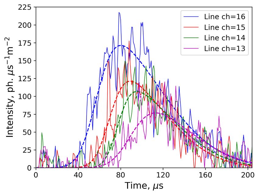
Figure 2. Light curve of the event TUS170915 and its SkewGauss approximation. Inset: Pixel map of
selected pixels and reconstructed track.

 The reconstruction of the light curves of the others EAS-like TUS events (the results are given
in section 3) gives the FDHM 50–70 s, and the asymmetry varying from 1.5 to 2.2. Estimates of
the amplitude of the signals also have significant variations.
 As mentioned above, the time shifts of the peak of the pixel’s signal can be interpreted as a
movement of a relativistic luminous compact object (in comparison to the resolution of the detector).
To determine the origin of the EAS-like events, it is important to reconstruct the arrival direction
of these objects.

1.2 Arrival direction

The optical system of the detector projects the movement of the source object onto the image’s
movement along the track on a focal plane. In the case of ideal (aberration-free) optics, the speed
of the point-like image is related to the apparent angular velocity of the light source by means
of the focal distance , = · .
 If the point-like light source moves in the atmosphere at a constant speed along a rectilinear
path, its image will also move along the rectilinear track on the focal plane. More precisely, the
track is formed by non-aberration points (we will call them “track points”), the structure of the
whole image depends on the point spread function (PSF) of the optics. The direction of motion
of the luminous object (arrival direction) can be determined by calculating the components of the

 –4–

speed of the non-aberration point along the track.
 In the local coordinate system, the direction of arrival Ω® can be set using azimuth and zenith
 ® = {sin cos , sin sin , cos } (Ω
 angles: Ω ® directs opposite to velocity of the source).
 If we denote by the angle between Ω ® and line of sight ®, the angular motion of the source
can be expressed through the speed of the source and the distance from it to the detector :
 • Non-relativistic sources (  ): = sin 

 • Relativistic sources ( ∼ ): = sin /(1 + 
 cos )

 • Ultra-relativistic sources ( ≈ ): = tan( /2)
 When observed in nadir, ≈ . For off-axis events, cos = cos cos − cos( ) sin sin ,
where is the field angle and is the angle between Ω ® and ® projected onto the ground.
 For a small , the difference between and can be estimated as a small correction. Thus for
ultra-relativistic sources in the local geographical coordinate system, we finally find:

 = Φdet − atan( / ), = 2 atan( / 0 ) + cos( ) (1.1)

with 0 = / and Φdet is the azimuth direction of the detector movement. For the TUS detector,
 0 = 0.9 mm/ s at = 500 km (or approximately 1 pixel per 20 GTUs) and the heading angle
Φdet ∼ −160◦ for all six EAS-like events.
 It follows from (1.1) that the movement along the track is non-uniform, however as the only
brightest part of the track could be detected, the variation in speed can be ignored. So to estimate
the zenith angle, we can substitute
 √︁ into equation (1.1) for parameters , and their values at
maximum point, so tan ≈ m2 + m2 / , tan ≈ m / m , where ( m , m ) are coordinates of the
maximum point.
 An important advantage of the orbital detection is its weak dependence to the height of the
source. Indeed, to calculate the angle with 5% accuracy, it is sufficient to know with the same
accuracy, i.e. at accuracy 10 km for the satellite’s orbit ∼ 500 km. At the same time due to the
exponential decrease in air density with altitude, the glow is localized in the lower layers of the
atmosphere. For example, the height of the EAS maximum with an energy ∼ 1020 eV does not
exceed 15 km up to = 80◦ .
 The application of classical track reconstruction methods in this case is complicated by several
reasons: a small number of track pixels, a large size and asymmetry of the PSF, and a significant
uncertainty in the sensitivity of channels and PSF. For example, one can track the movement of the
image centroid by approximating the hit pixel signals at each GTU with a suitable parameterized
distribution. However, since the error in the localization of the centroid is comparable to the size
of the entire image, for some events the displacement cannot be detected, and in some cases, on the
contrary, the instantaneous velocity varies greatly from GTU to GTU. Therefore, in [6], the Linear
Track Algorithm heuristic (LTA) was proposed, which can be used to reconstruct track parameters
in such an uncertainty situation.
 In the following, section 2 provides an analysis of the accuracy of the LTA, and section 3
presents the results of its application to the EAS-like events registered by the TUS. Finally, in
section 4, localization of the reconstructed tracks allows us to hypothesize the origin of these
events.

 –5–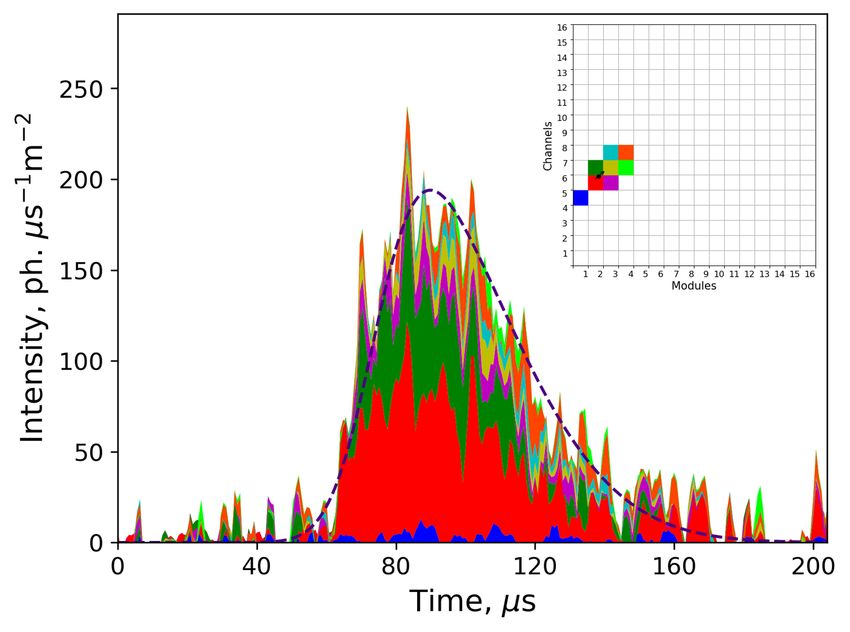

2 LTA reconstruction scheme

The problem of reconstructing the image of the EAS fluorescence as a linear track on the focal surface
of an orbital detector was studied in detail in a number of works of the JEM-EUSO collaboration,
[7], [9]. Two requirements are necessary to use the methods proposed in these papers: 1) matching
of the optics and the photodetector and 2) a large number of hit pixels in the image. Here by
matching, we mean that the characteristic size of the (instantaneous) image is approximately equal
to the size of the photo sensor, which leads to a fairly accurate localization of the track point. A
large number of pixels is required for small statistical errors of resulting estimates (for this reason,
the accuracy of the arrival direction reconstruction decreases significantly with decreasing zenith
angle). However, both of these requirements are not met in the case of the TUS detector. The size
of the PSF is rather big so the instant image is distributed over 4-6 neighboring pixels. The track
length does not significantly exceed its “thickness” (as we will see later, this is due to the fact that
the recorded events have zenith angles of 30◦ and less).
 In an alternative approach, reconstruction of the EAS-like event can be achieved in a probabilis-
tic model by Bayesian inference [10] of the posterior distribution to unknown track { m , m , m , , }
and light curve parameters { m , FDHM, Asymmetry}. The following information on the signals in
the hit pixels is used in this case: the coordinates of the centers of these pixels { , }, = 1, ..., ,
and the values of the active signal in them { ( )} ( is the number of selected pixels, is
the GTU index). The active signal itself must be obtained by subtracting the background and
subsequent normalization to the channel sensitivity. The sensitivity coefficients and PSF are used as
a priori information in such a probabilistic approach. Unfortunately, this information is known with
large uncertainty. The sensitivity of individual channels changed a lot during the operation of the
detector in orbit (for more details, see [6]) and it has to be estimated indirectly during experiment
by stationary waveforms analyses. Lastly, the PSF of the TUS mirror varies greatly throughout the
photodetector FOV, both in size and shape.

2.1 LTA and its hyperparameters
In the situation of such a strong uncertainty of a priori information, it is more efficient to develop
a heuristic approach for track reconstruction. The idea of this approach, first described in [11]
and then modified in [6], is to make an approximation of the time dependence of the track points
coordinates, ( ) = m + ( − m ), according to the distribution of the coordinates of the
centers of hit pixels: m is estimated by the light curve fit, the parameters , m are selected by
minimizing the weighted sum of the squared deviations (and similarly for ( )). To reduce the
approximation roughness associated with pixelization, the corresponding signal values ( ) are
used as the weights of each “point”. More precisely, the algorithm includes the hyperparameter
 exp that controls a dependence of the weight on the signal, ∼ [ ˜ ( )] exp , where ˜ ( ) is
(smoothed) value of the signal at time .
 Another important feature of this method, called Linear Track Algorithm (LTA), is the selection
of a suitable time “activity window” for each signal. The very wide window leads to a systematic
underestimation of while a small window corresponds to big variation of the results (see below).
In this paper, it is proposed to control the size of the activity window by the second hyperparameter
of the algorithm - the activity threshold act . Thus, in LTA, the following sum is minimized

 –6–

2 ( )
 ∑︁
 ∑︁
 [ ˜ ( )] exp · [ m + ( − m ) − ] 2 , (2.1)
 =1 1 ( )

by parameters and m . The boundaries of the activity window 1 ( ), 2 ( ) are determined so
that ˜ ( ) exceeds the threshold act over the entire (maximum) interval [ 1 ( ) , 2 ( ) ].
 Thus, the operation of the LTA is controlled by two hyperparameters, exp and act , the
dependence of the reconstruction results and the choice of their optimal values was carried out on
a simulated events data base.

2.2 Simulated events reconstruction
To set the hyperparameters of the algorithm and to evaluate the accuracy of its predictions (recon-
struction accuracy), we use a data base of simulated events with characteristics which are similar to
the TUS EAS-like events. This determines the choice of the range of zenith angles, the duration and
asymmetry of the light curve and the characteristic signal-to-noise ratio (associated with the number
of triggered pixels). For convenience, the track and light curve parametrization of the simulated
events were performed directly on focal plane of the photodetector. To generate a reference data
base (RDB) with 1000 simulated events, we choose the following parameters distribution2:
 • Track: velocity projections , corresponding to 0 ∼ U [−180◦ , +180◦ ], 0 ∼ U [20◦ , 40◦ ].

 • Light Curve: Skew-Gauss function with uniformly distributed scale and shape parameters
 corresponding to FDHM∈ [52, 80] s and Asymmetry∈ [1.5, 2.3].
 The pixel distribution of the signal was performed using a 2D isotropic Gaussian PSF. The
characteristic size of the PSF was selected to correspond to the control optical tests [12]. Measure-
ments showed that the diameter of the circle of confusion with 70% of full energy of the image 70
varies from 15 mm in the center of the photodetector to 23-27 mm at the edge. Since all the TUS
events covered in this article are localized close to the edge of the FOV, for the RDB we selected
 70 ∼ U [22.5, 25.5] mm (which corresponds to the range 1.5-1.7 in pixel size units). In order to
take into account the uncertainty in the channel response, each sensitivity coefficient was varied
due to a Gaussian distribution with a 20% standard deviation.
 The choice of the signal amplitude, background level and the pixel selection criteria were
carried out, so that the number of such channels and the signal-to-noise ratio were comparable with
those obtained for the TUS events. Accordingly, we fixed an amplitude m = 100 a.u. (arbitrary
units) and the noise noise = 5 a.u., so the pixel selection by their amplitude (both as MA(8)
and as Gauss fit) at the level sel = 4 a.u. gives the number of the hit pixels averaged on RDB
 sel = 7.0 ± 1.1.
 The Signal-to-Noise ratio for the selected pixels is presented in table 2, for three variants of
the ’signal’: the amplitude of the Gauss fit, the signal integrated in 8 GTUs, and the signal inside
FDHM interval (as a ratio to the corresponding standard deviation of the background).
 The result of the arrival direction reconstruction of an individual simulated event can be
presented as errors – the differences between the reconstructed angles and their true values, Δ ≡
 rec − 0 and Δ ≡ rec − 0 .
 2 ∼ U [ , ] means uniformly distributed on the interval [ , ].

 –7–

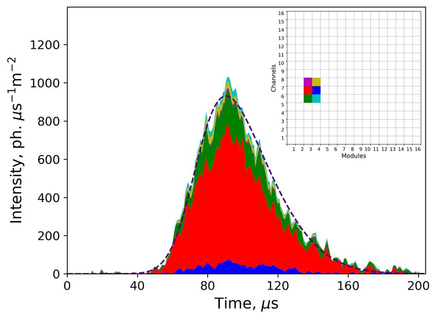
Table 2. Signal to Noise ratio (SNR) in first 7 selected pixels (sorted by amplitude) averaged on RDB for
 sel = 4, noise = 5, the three variants correspond to fit amplitude, MA(8) selection and FDHM signal (see
text).

 SNR: #1 #2 #3 #4 #5 #6 #7
 p / noise 7.4 5.2 3.7 2.8 1.8 1.3 0.8
 √
 8 /( noise 8) 22.8 16.3 12.3 9.9 6.7 5.0 3.3
 √
 /( noise Δ ) 46.1 32.5 23.7 18.1 11.1 7.8 4.9

 10 10

 5 5
 , deg.

 , deg.
 0 0
 ,

 ,
 -5 -5

 -10 -10
 0.5 1 1.5 2 2 4 6 8 10
 nexp qact

Figure 3. LTA accuracy as a function of exponent exp (left, act = 5 a.u.) and as a function of activity
threshold act (right, exp = 1.5). Blue colors for -errors, red ones for -errors.

 Reconstruction of the entire RDB allows one to evaluate the statistical accuracy (or reliability)
of the method. For example, at fixed values of the LTA hyperparameters it can be presented as a
histogram of errors. The two main characteristics of the error distribution are the bias and width
of the error histogram, which can be taken as the mean values of Δ or Δ and their standard
deviations, respectively.
 To study how the accuracy of the LTA depends on the hyperparameter setting, error curves
were plotted for RDB – the bias and width dependencies on exp and act for both angles, figure 3
(the lines correspond to the mean values, the filled areas are ±1 standard deviation, blue color for
Δ , red one for Δ ). The left panel of the figure shows the error curves for the exponent parameter,
which suggests an optimal choice for exp . The position of the minimum of the errors, calculated
 √︁
as RMS = bias2 + width2 , depends on the sensitivity variation, but is always close to exp ≈ 1.5.
In further work, we fix the hyperparameter of the exponent at this value.
 The optimal values of the activity threshold act for reconstructing the azimuth angle lie in the
region of small values, see the right panel of figure 3, while for the zenith angle this region has a
significant bias (underestimating the speed along the track). On the other hand, increasing act , the
number of approximation points decreases, which leads to a wider error distribution.

2.3 Event-by-event reconstruction
The optimal activity threshold cannot be fixed on one specific value - it will change when varying,
for example, the signal-to-noise ratio or selection procedure. Therefore the final choice of the act

 –8–

Figure 4. Typical behaviour of a reconstruction curve for simulated event: -curve with AV region at small
threshold (left panel) and -curve with ZGP (right panel)

Figure 5. Error Histograms for RDB for angle with the AV-prescriptions (left panel) and for angle for
ZGP-prescription (right panel). Δ = (0.2 ± 5.3) ◦ , Δ = (0.9 ± 4.7) ◦ .

should be carried out in event-by-event basis and rely on the behavior of reconstruction curves, i.e.
the reconstructed angle dependence on the activity threshold. The typical behavior for the RDB
events reconstruction curves are shown in figure 4.
 The shape of the -curve has a region at small act with an asymptotic behaviour of the curve,
the region with small rec variations. In the following, we called the choice of this asymptotic
value for azimuth angle as AV-prescription. On the other hand, the reconstruction curve can have
different shape with several local maxima. The first maximum (with the smallest act ) we called
zero gradient point (ZGP), and use this ZGP-prescription to choose the rec .
 Histograms of the angle reconstruction for RDB events are presented on figure 5. AV-
prescription for Δ -histogram gives approximately zero bias, Δ = (0.2 ± 5.3) ◦ (here we use
notation mean±std). By contrast, Δ -histogram constructed in accordance with ZGP-prescription,
has a noticeable bias, Δ = (0.9 ± 4.7) ◦ . However, this bias depend strongly on data base parame-
ters, so we can not fix this shifts in the -reconstruction procedure. Therefore, we will use the RMS
errors as a measure of the LTA uncertainty, Δ = 5.3◦ , Δ = 4.8◦ .

 –9–

3 TUS events reconstruction

When reconstructing the TUS events, the following sequence of steps is performed:

 • Light curve reconstruction: m , m , FDHM, Asymmetry estimations by SkewGauss fit of
 the sum of all active signals.

 • Track reconstruction by LTA: / , m , m by AV-prescription, by ZGP-prescription.

 • Arrival direction: and from (1.1), and corresponding direction on celestial sphere with
 1st Equatorial coordinates.

 The results of the reconstruction of the light curves and the apparent kinematic parameters of
the source movement for all EAS-like TUS events are presented in table 3. The light curves and
corresponding pixel maps with reconstructed track (black arrow) are shown3 on figure 6.

Table 3. Light curve reconstruction (amplitude, duration and asymmetry coefficient) and apparent movement
parameters.

 Events max , ph. m−2 s−1 FDHM, s Asymmetry , rad/s / Δ , km
 TUS161003 205 49.4 1.56 210 0.34 10.0
 TUS161031 121 61.8 2.18 122 0.20 7.4
 TUS170915 442 72.0 1.69 173 0.28 12.1
 TUS171010 452 62.8 1.82 179 0.28 10.6
 TUS171029a 193 46.6 1.59 112 0.18 4.9
 TUS171029b 443 63.8 1.61 81 0.13 4.9

 Part of the luminescence cannot be recognized due to rather large PSF, so the reconstruction
gives the deformed shape of the light curve. The estimates of the m , FDHM, and Asymmetry
have noticeable errors, e.g. m is lower estimate of the amplitude. A significant contribution to the
uncertainty of these quantities is also made by the inaccuracy of the absolute sensitivity calibration
(see below about “red” pixels).
 The angular velocity = / of the line of sight to the source characterizes its movement
in the picture plane only and does not depend on the distance to the source. On the contrary, the
apparent linear velocity = and track length Δ = · 2FDHM (both projected onto the picture
plane) were obtained under the assumption that the distance to the source coincides with the height
of the satellite’s orbit (varies from 475 to 495 km). One can see that all events are relativistic.
 When reconstructing the TUS events in comparison with simulated ones, two conditions, 1)
strong irregularity in the distribution of channel sensitivities, and 2) asymmetry of PSF (non-
isotropic and non-uniform) should be taken into account. Both primarily affect the estimates of the
velocity components of movement along the track.
 The existence of channels with low sensitivity leads to skipping signals in some cases, and
to not reliable fitting in others. In addition, the calibration of less sensitive channels has the
largest uncertainty (for several channels, the sensitivity coefficients are known with an accuracy of
 3Light curve of the TUS170915 is presented on figure 2, and of the TUS161003 - in our previous paper [6].

 – 10 –

Figure 6. TUS events light curves: top – TUS161031, TUS171010, bottom – TUS171029a, TUS171029b.

hundreds of percent). We will call such weakly sensitive channels “red”. In those cases when the
selection procedure finds “red” pixels, we plot reconstruction curves for a set of sensitivity values
and estimate the variability of the AV- and ZGP-values (see below).
 The asymmetry of the PSF can lead to a significant systematic bias in the speed estimation of
the image propagation along the track. For example, an off-axis coma-type aberration shifts the
image centroid in a radial direction relative to the position of the non-aberration track point. This
stretches the track and leads to an overestimation of speed by the LTA method. It is very difficult to
quantify this effect. Reconstruction of simulated events with a convolution of the coma and Gauss
distributions (with the TUS mirror parameters) as PSF showed that the systematic bias in can
vary from 0 to +3.5◦ depending on the location of the track on the pixel map. To partially reduce
this bias, the signals fit should be performed by an asymmetric function that selects the main part
of the signal not near the centroid, but close to the track point. We use the SkewGauss function
to fit the EAS-like TUS event signals (with a limited range of shape and scale parameter). So
besides the methodical inaccuracy, an additional event specific contribution to the uncertainty of
the reconstructed angle should be taking into account, we name it the measurement error.
 In the following, the reconstruction of the arrival directions was made under the assumption
that the total speed of the source is equal to the speed of light. The results are presented in table 4,
where the direction is expressed both as the ( , ) angles of the local coordinate system, and in the

 – 11 –

Table 4. Arrival direction in local ( , ) and Equatorial coordinate systems ( , ). Number of weakly
sensitive channels (’reds’), measurement error for and special feature of registration are presented in the
last column (see the text for details).

 Events , ◦ , ◦ , ◦ , ◦ Comments
 TUS161003 144 38 308 65
 TUS161031 166 26 343 83 2 reds, Δ mes = 2◦
 TUS170915 86 28 311 33 Δ mes = 1◦
 TUS171010 231 28 41 49
 TUS171029a 333 17 35 19 1 red, Δ mes < 1◦
 TUS171029b 16 11 33 55 boundary event

Figure 7. AV-region determination: left panel - for the event TUS170915, right panel - for the event
TUS161031 (two variants, see text).

Equatorial coordinate system (right ascension and declination ). The directions of arrival of the
sources of the registered events are not concentrated near any one direction, but are distributed over
a significant part of the celestial sphere.
 The TUS170915 is an example of an event whose direction of arrival can be determined with
a high degree of reliability. 12 pixels were selected to build the reconstruction curves in this case.
The shape of the -curve is similar to the typical one with definite ZGP. However, in contrast to the
simulated -curves, the real one (figure 7, left panel) has a small gradient at the smallest threshold
 act , which makes it difficult to determine the AV region. In fact, the presence of such a gradient
is typical of EAS-like TUS events and can be explained by the existence of significant asymmetry
of pixel signals caused by the contribution of coma aberration due to PSF. For the TUS170915,
this “deformation” of the -curve is insignificant, and the ’truth’ AV region can be detected near
 act = 10 (see the dashed line in figure 7). So for the TUS170915, the measurement error is
estimated as Δ mes = 1◦ .
 For the event TUS161031, only six selected channels have a reliably sensitivity coefficients,
two more are “red”. Accordingly, a set of reconstruction curves was used with different values of the
sensitivity for the red channels. Right panel of figure 7 shows -curves for two limit values ( -curves
have a typical shape and vary slightly). The measurement error is estimated as Δ mes = 2◦ .

 – 12 –

A weakly sensitive channel is also found in the event TUS171029a. However, in this case, the
reconstruction curves practically do not change when the sensitivity coefficient varies over a wide
range for this red channel. Therefore, the measurement error is not more than 1◦ .
 Particular difficulty arises during the reconstruction of the event TUS171029b. It is located at
the edge of the detector FOV and the analysis of the signals shows that part of the track lies outside,
and therefore has not been registered (see the inset on the bottom-right panel in figure 6). The
presence of a signal outside the FOV can “tilt” the track during reconstruction. In addition, in such
cases of “boundary events”, the LTA underestimates the determination of a speed of movement
along the track. Thus, a measurement error is present here for both the azimuth and zenith angles,
however, it is currently not possible to evaluate it (so azimuth reconstructions in this case are
qualitative rather than quantitative).
 Finally, in the two remaining events, TUS171010 and TUS161003, the above problems are not
observed: the large number of selected pixels with relatively high sensitivity allows us to estimate
the angles without additional error. In [6], the zenith angle of the TUS161003 was estimated 6◦
more, a consequences of using a less reliable version of LTA with a relative rather than an absolute
threshold act . A more thorough analysis showed that such an LTA option in some cases can lead
to large systematic shifts in the -estimation.

4 Discussion

We emphasize that the choice of these six events as representatives of the EAS-like class was
determined by two features: the characteristic shape and duration of the light curve and the presence
of a noticeable time displacement of the channel signal peaks. This last cut can be interpreted as
the movement of a relativistic radiation source. The LTA has been tested only on events with such
a movement. A number of recorded events partially suited to these properties were not analyzed in
this work. For example, the figure 8 shows the light curve of another event registered 27.06.2017
above the USA (32.89S, 100.99W), for which, despite the presence of 6 hit pixels, it is not possible
to establish the source movement: LTA reconstruction leads to < 1◦ , and the image itself is most
likely caused by the PSF effect.
 On the other hand, a lot of events with EAS-like light curves were rejected due to the small
number of hit pixels since the reconstruction is unreliable in this case.
 The formulas presented in section 1 for the non-relativistic, relativistic, and ultra-relativistic
cases can be unified as
 sin 0
 / = , tan( 0 ) = / , (4.1)
 sin( − 0 )
For a fixed value of the apparent linear velocity , different geometries of the track correspond to a
different speeds of a source. There are no tracks with < 2 0 .
 A minimum speed of the moving object, min = sin 0 , corresponds to up-going track at an
angle of /2 + 0 with respect to the line of sight. For typical value of / = 0.25 from the table 3,
we have 0 ≈ 14◦ and min / = 0.24.
 For all other arrival directions, two possible correspond to the observed apparent velocity .
It is important to emphasize that for all 6 estimations of the and any variant of the arrival direction
the motion of the source is relativistic (as ≥ min ).

 – 13 –

Figure 8. One of the TUS events with expected EAS light curve but without peak movement.

 It is rather difficult to assume the presence of a relativistic source of UV radiation, with speed
different from the speed of light, for example, in the range from 0.2 to 0.9 . In the ultra-relativistic
limit, the movement can be either down-going, → 2 0 , or up-going vertically along the line of
sight, → . The second scenario, however, cannot be realized in our events, since the observed
luminescence track length would correspond to a very large track in the atmosphere (more than
100 km), the region where UV radiation cannot be deliberately produced. So the most probable
kinematics of EAS-like TUS events corresponds to scenario with = 2 0 which we’ve used in the
LTA reconstruction.
 Using the Google Maps resource4, an analysis was made of objects localized at the track
location of each of the 6 events. It turned out that in all cases there is one or more airports in the
immediate vicinity of the track. In particular, as shown in the figure 9, the TUS170915 track (the
dark magenta line with a circle) is a continuation of the runway of the Craig Moffat County Airport
within the accuracy of the reconstruction. The white squares in the figure show the fields of view
of 12 hit pixels (∼ 5 × 5 km2 ), the magenta circle indicates the position of the maximum.
 In this regard, an assumption was made about the anthropogenic origin of the source of all the
events considered in this article. More precisely, a hypothesis was put forward on the correlation
in the position and direction of runways and the observed track. Airport Runway hypothesis means
that the track of the event coincides with the continuation of the airport runway which involves two
conditions: 1) small difference Δ in track and runway directions, and 2) their close location.
 The accuracy of the angle between the projection of the direction of the track onto the Earth’s
surface and the direction of the runway Δ corresponds to the accuracy of the reconstruction of
the azimuth angle . In addition to the methodical component (∼ ±5◦ ), Δ has measurement
error varying from event to event. The main uncertainty in the position of the track is due to the
inaccuracy of the time stamp of the registration of the event. In fact, the trigger time stamp was

 4https://www.google.com/earth/

 – 14 –

Figure 9. Google Earth map for the event TUS170915. The yellow line corresponds to the runway of the
Craig Moffat County airport. The reconstructed track presented by magenta line with a circle (’maximum
point’).

transmitted with an accuracy of 1 second, which corresponds to shifts of the detector FOV along the
direction of motion by about 8 km (cf. with 5 km size of pixel field of view). In addition, sometimes
de-synchronization occurred during the TUS operation, which led to uncontrollable time shifts Δ 
of 1-3 seconds.
 For each EAS-like event we are looking for the closest airport and estimate Δ angle between
track and runway directions and probable time shifts Δ . The tracks of five of the six EAS-like
events are similar in location and direction to the runway:

 • Event TUS161031: Sparrevohn AFC Airport with LRRS, Δ = 10◦ , Δ < 0.5 s (track from
 or above runway).

 • Event TUS170915: Craig Moffat County Airport, Δ ≈ 0◦ , Δ < 0.5 s (from runway).

 • Event TUS171010, two candidates: 1) Cherry Point Mcas Airport, Δ < 5◦ , Δ ≈ +2 s
 (from runway) or 2) Coastal Carolina Regional Airport, Δ = 15◦ , Δ ≈ −1 s (from or above
 runway).

 • Event TUS171029a: Winslow-Lindbergh Regional Airport, Δ ≈ 25◦ (from runway), Δ ≈
 −0.5 s (low accuracy of track reconstruction).

 • Event TUS171029b: Tin City Airport (with LRRS), Δ = 20◦ , Δ ≈ 0 s (above runway). This
 is “boundary event” with a big part of the signal outside the TUS FOV.

We can conclude that in the first three cases, the hypothesis is confirmed within the accuracy of
measurements. In the last two events, the additional error in Δ can be explained by a peculiar
properties of the reconstruction.

 – 15 –

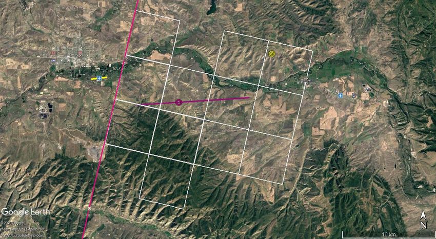
The only event that clearly does not correspond to the hypothesis is one which detailed analysis
was carried out in [6]:

 • Event TUS161003: Christison Airport, Δ ≈ 45◦ , Δ ≈ −1 s (to runway).

 In the vicinity of the event there are a large number of local airports, however, the orientation of
all their runways is very different from the direction of the track. It is interesting to note that the only
nearby sufficiently large Rochester International Airport has the “correct” orientation (Δ < 5◦ ),
but it is shifted (along the detector movement) by 40 km.
 There are several possible explanations for this direction–location correlation. On the one
hand, the source of linearly aligned UV light can be aircraft warning lights systems located along
the direction of approach to a runway. In addition, mounted on aircraft landing lights illuminate
the terrain and runway ahead during takeoff and landing. This illumination is bright white, forward
and downward facing lights on the front of an aircraft (the landing lights of large aircraft can easily
be seen by other aircraft over 100 miles away).
 Unfortunately, in any of these variants it is rather difficult to explain the characteristic spatio-
temporal pattern of events recorded by the TUS: a light curve with a duration of about 100 s and
a signal peak displacement with an apparent speed of several tens of percent of the speed of light.
 It is well known that transient UV flashes can also be observed when an electromagnetic
pulse (EMP) penetrates into the lower layers of the ionosphere, [13]. In particular, the appearance
of the so-called elves, large-scale ring-shaped optical flares at an altitude of 80-90 km, with a
characteristic glow time of about 1 ms, is explained by an EMP generated by lightning discharge,
[14], [15]. During its operation, the TUS detector registered 25 elves (including the so-called
double elves), [16]. For this type of events, the characteristic duration of the signal in a channel was
also several tens of microseconds, but its amplitude was more than an order of magnitude higher,
and the whole image of the elve occupied most of the entire FOV.
 Several different types of radio transmitting stations are located near airports5. VHF omnidi-
rectional range (VOR) is used to determine the azimuth of the direction of movement of the aircraft
(often combined with Distance Measuring Equipment, DME). VOR is a phased antenna array to
send a highly directional signal that rotates 30 times a second. For each of the EAS-like TUS events,
we have identified the nearest VOR station using the resource https://www.airnav.com. For
example, in figure 9, Hayden VOR/DME station (40.5201◦ N, 107.3049◦ W) is marked with a yellow
circle, so the TUS170915 track is located exactly between (with an accuracy of an acceptable offset
within 0.5 s) the runway and the VOR.
 Interestingly, despite the directions of the TUS17102a track and the runway do not coincide,
Winslow VORTAC6 station (35.0616◦ N, 110.7950◦ W) is located at the intersection of these two
directions, see figure 10. For all EAS-like TUS events, a VOR station was found in the immediate
vicinity of the event maximum. Specifically for the TUS171010 event, New Bern VOR/DME
(35.0731◦ N, 77.0451◦ W) is located right next to the Coastal Carolina Regional Airport. The
only exception is again the TUS161003 event: here VOR/DME is located on the extension of the
Rochester International Airport runway, i.e. more than 30 km from the reconstructed track.

 5https://en.wikipedia.org/wiki/Instrument_landing_system
 6VORTAC is a collocated VOR and Tactical Air Navigation station.

 – 16 –

Figure 10. Google Earth map for the event TUS17102a. The yellow line corresponds to the runway of the
Winslow-Lindberg Airport, and yellow circle to the Winslow VORTAC station.

 However, the hypothesis of the appearance of a EAS-like events by means of “highlighting”
the lower layers of the ionosphere with a VOR radio signal has many shortcomings. The main
energy of the lightning EMP which generates elve is carried in the VLF (3-30 kHz) range, while
the radio signal generated by the VOR station has a frequency in the 108-118 MHz range, and the
VOR transmitter power is much weaker to the lightning. In addition, in this case the apparent speed
of movement when observed from orbit must exceed the speed of light.

5 Conclusions

The orbital detector TUS, due to the use of a large-area mirror-concentrator and a highly sensitive
photodetector, is able to register short-term UV signals (flashes) that are inaccessible to other
devices. In this work, special attention was paid to the class of so-called EAS-like events with a
characteristic light curve duration of about 100 s and a noticeable spatial displacement of the peak
of the signal (“track”). A total of six such events were selected. Reconstruction of such events is
complicated by a short track length, an asymmetry of the image, and an uncertainty in the sensitivity
distribution of the TUS channels. The new method of reconstruction of the kinematic parameters of
such events was developed and made it possible to determine the direction of arrival of their source
- it corresponds to downward relativistic movement with zenith angles from 10◦ to 40◦ .
 Despite their name, it is difficult to associate such events with the EAS fluorescence because
of significant signal intensity (it should correspond to ZeV primary). All six events were located
over the mainland of the United States. Moreover, the reconstructed tracks revealed a correlation
with the runways of the airports. This allowed us to propose several possible hypothesis for the
anthropogenic origin of the sources of these phenomena, including aircraft landing lights and the
effect of radio pulses from VOR stations on the ionosphere, each of which faces difficulties in

 – 17 –

interpreting all the revealed patterns. Detailed analysis of these and other possible hypotheses of
the origin of the EAS-like events will be carried out in another paper.
 The method developed in this work provides the reliable determination of kinematic parameters
of the track-like events, registered with low spatial resolution. For the final solution of the riddle
of the origin of events of this type, it is extremely important to increase their statistics. In this, the
analysis of data from the new orbital detector Mini-EUSO [17] can play a key role. In the case
of anthropogenic origin of EAS-like events, the determination of their characteristics will make it
possible to exclude them from further analysis in next-generation space missions K-EUSO [18] and
POEMMA [19] (or even implement suitable selection criteria into trigger systems).

Acknowledgments

The authors are grateful to Mikhail Zotov for his very important work in the search and classification
of TUS events, and to Pavel Klimov and Boris Khrenov for a fruitful discussion of the results.
 Oliver Isac Ruiz Hernandez is grateful to Oscar Martínez Bravo by his guidance and continu-
ously supervision on his process to become a researcher.
 The work was done with partial financial support from the State Space Corporation ROSCOS-
MOS, M.V. Lomonosov Moscow State University through its “Prospects for Development” program
(“Perspektivnye Napravleniya Razvitiya”). Also with partial financial support of the Vicerrectoría
de Investigación y Estudios de Posgrado (VIEP-BUAP).

References
 [1] R. Benson and J. Linsley, Satellite observation of cosmic ray air showers, International Cosmic Ray
 Conference 8 (1981) 145–148.
 [2] P. A. Klimov, M. I. Panasyuk, B. A. Khrenov, G. K. Garipov, N. N. Kalmykov, V. L. Petrov et al., The
 TUS detector of extreme energy cosmic rays on board the Lomonosov satellite, Space Science Reviews
 (8, 2017) 1–17.
 [3] B. A. Khrenov, P. A. Klimov, M. I. Panasyuk, S. A. Sharakin, L. G. Tkachev, M. Y. Zotov et al., First
 results from the TUS orbital detector in the extensive air shower mode, J. of Cosmology and
 Astroparticle Physics 2017 (2017) 006, [1704.07704].
 [4] S. V. Biktemerova, A. A. Botvinko, N. P. Chirskaya, V. E. Eremeev, G. K. Garipov, V. M. Grebenyuk
 et al., Search for extreme energy cosmic ray candidates in the TUS orbital experiment data, ArXiv
 e-prints (June, 2017) , [arXiv:1706.05369].
 [5] M. Bertaina, A. Castellina, R. Cremonini, F. Fenu, P. Klimov, A. Salsi et al., Search for extreme
 energy cosmic rays with the TUS orbital telescope and comparison with ESAF, in European Physical
 Journal Web of Conferences, vol. 210 of European Physical Journal Web of Conferences, p. 06006,
 Oct, 2019, DOI.
 [6] B. A. Khrenov, G. K. Garipov, M. A. Kaznacheeva, P. A. Klimov, M. I. Panasyuk, V. L. Petrov et al.,
 An extensive-air-shower-like event registered with the TUS orbital detector, J. Cosmology Astropart.
 Physics 2020 (Mar., 2020) 033, [1907.06028].
 [7] C. Berat, S. Bottai, D. De Marco, S. Moreggia, D. Naumov, M. Pallavicini et al., Full simulation of
 space-based extensive air showers detectors with ESAF, Astroparticle Physics 33 (May, 2010)
 221–247, [arXiv:0907.5275].

 – 18 –

[8] A. Azzalini and A. Capitanio, The Skew-Normal and Related Families, Cambridge University Press
 (2014) 24–54.
 [9] JEM-EUSO collaboration, S. Biktemerova, A. Guzman and T. Mernik, Performances of JEM-EUSO:
 angular reconstruction, Exper. Astron. 40 (2015) 153–177.
[10] D. Sivia and J. Skilling, Data Analysis: A Bayesian Tutorial. Oxford science publications. OUP
 Oxford, 2006.
[11] L. Tkachev and Lomonosov-UHECR/TLE Collaboration, Search for EAS candidates with the
 TUS/Lomonosov orbital experiment: results of preliminary data reconstruction and analysis, in
 Proceedings of Science (ICRC2017), no. 527, 2017.
[12] TUS collaboration, P. Klimov et al., Ultra high energy cosmic rays detector TUS on-board
 Lomonosov satellite, in Proceedings, 33rd International Cosmic Ray Conference (ICRC2013): Rio de
 Janeiro, Brazil, July 2-9, 2013, p. 0406, 2013.
[13] C. T. R. Wilson, The electric field of a thundercloud and some of its effects, Proceedings of the
 Physical Society of London 37 (jan, 1924) 32D–37D.
[14] U. S. Inan, W. A. Sampson and Y. N. Taranenko, Space-time structure of optical flashes and
 ionization changes produced by lighting-emp, Geophysical Research Letters 23 (1996) 133–136,
 [https://agupubs.onlinelibrary.wiley.com/doi/pdf/10.1029/95GL03816].
[15] U. S. Inan, S. A. Cummer and R. A. Marshall, A survey of elf and vlf research on lightning-ionosphere
 interactions and causative discharges, Journal of Geophysical Research: Space Physics 115 (2010) ,
 [https://agupubs.onlinelibrary.wiley.com/doi/pdf/10.1029/2009JA014775].
[16] P. Klimov, B. Khrenov, M. Kaznacheeva, G. Garipov, M. Panasyuk, V. Petrov et al., Remote sensing of
 the atmosphere by the ultraviolet detector tus onboard the lomonosov satellite, Remote Sensing 11
 (2019) .
[17] F. Capel, A. Belov, M. Casolino and P. Klimov, Mini-EUSO: A high resolution detector for the study
 of terrestrial and cosmic UV emission from the International Space Station, Advances in Space
 Research 62 (2018) 2954–2965, [1709.00405].
[18] P. Klimov and Lomonosov-UHECR/TLE Collaboration, Status of the KLYPVE-EUSO detector for
 EECR study on board the ISS, in Proceedings of Science (ICRC2017), no. 412, 2017.
[19] A. V. Olinto et al., POEMMA: Probe Of Extreme Multi-Messenger Astrophysics, PoS (2017) 542,
 [arXiv:1708.07599].

 – 19 –