JT gravity from holographic reduction of 3D asymptotically flat spacetime - Springer Link
←
→
Page content transcription
If your browser does not render page correctly, please read the page content below
Published for SISSA by         Springer
                                                                  Received: December 5, 2022
                                                                   Accepted: January 3, 2023
                                                                  Published: January 25, 2023

JT gravity from holographic reduction of 3D

                                                                                                JHEP01(2023)138
asymptotically flat spacetime

Arindam Bhattacharjeea,b and Muktajyoti Sahac
a
  Harish-Chandra Research Institute,
  Chhatnag Road, Jhunsi, Prayagraj 211019, India
b
  Homi Bhabha National Institute,
  Training School Complex, Anushaktinagar, Mumbai 400094, India
c
  Indian Institute of Science Education and Research Bhopal,
  Bhopal Bypass, Bhauri, Bhopal 462066, India

    E-mail: arindamb.hep@gmail.com, muktajyoti17@iiserb.ac.in

Abstract: We attempt to understand the CFT1 structure underlying (2+1)D gravity in
flat spacetime via dimensional reduction. We observe that under superrotation, the hy-
perbolic (and dS2 ) slices of flat spacetime transform to asymptotically (A)dS2 slices. We
consider a wedge region bounded by two such surfaces as End-of-the-World branes and em-
ploy Wedge holography to perform holographic reduction. We show that once we consider
fluctuating branes, the localised theory on the branes is Jackiw-Teitelboim (JT) theory.
Finally, using the dual description of JT, we derive an 1D Schwarzian theory at the spatial
slice of null infinity. In this dual Celestial (nearly) CFT, the superrotation mode of 3D
plays the role of the Schwarzian derivative of the boundary time reparametrization mode.

Keywords: 2D Gravity, Gauge-Gravity Correspondence, Space-Time Symmetries

ArXiv ePrint: 2211.13415

Open Access, c The Authors.
                                                   https://doi.org/10.1007/JHEP01(2023)138
Article funded by SCOAP3 .
Contents
1 Introduction 1
2 Foliations and their relation to asymptotic symmetry 3
2.1 Foliations of flat spacetime 3
2.2 (2+1)D asymptotically flat spacetimes 4
2.3 Effect of superrotation on foliations 5
JHEP01(2023)138
3 Dimensional reduction of Einstein-Hilbert action 6
3.1 Wedge holography: a brief review 7
3.2 Reduction to rigid slices 7
3.3 Reduction to fluctuating AdS2 slices 9
3.3.1 Effective action for the whole hyperbolic patch 10
3.3.2 Fall-off condition for the dilaton 11
3.4 Fluctuating dS2 patch: analytic continuation 11
4 Boundary Schwarzian theory 12
4.1 Null boundary term for 3D gravity 12
4.1.1 General construction 12
4.1.2 Null boundary term from 3D asymptotically flat spaces 13
4.2 GHY term for 2D (A)dS2 slices 14
4.3 1D effective action: Schwarzian 15
5 Conclusions and outlook 16
1 Introduction
The nature of holography in flat spacetime has been a subject of intense study in recent
years (See [1–3] and references therein). Analysing the structure of asymptotic symmetries
in 4D flat spacetimes [4, 5], it has been argued [2] that the dual theory at the boundary is
a two dimensional CFT, termed Celestial CFT. More generally, it was argued that (d+1)
dimensional theory of gravity in asymptotically flat spacetime has a (d-1) dimensional CFT
description [6].
At first glance, this seems pretty straightforward. Since the Lorentz group of (d+1)
dimensional flat spacetime is SO(d, 1) which is also the global conformal group at (d-1)
dimensions. Thus every flat space amplitude, by virtue of being Lorentz invariant, is
also conformally invariant. This invariance can be made explicit when the amplitudes are
written in appropriate basis. The non-triviality comes while enhancing the global con-
formal invariance of the 4D amplitudes to full Virasoro invariance of the dual 2D CFT
–1–description [7]. These infinite dimensional symmetries are interpreted in the bulk as the
superrotation symmetries associated with subleading soft graviton theorem [8, 9]. Thus
the amplitudes of any quantum field theory which is coupled to gravity in the bulk are
constrained by Ward identities coming from the full Virasoro symmetry. This gives an ex-
traordinary advantage over the structure of generic gauge/gravity amplitudes and produce
new insights into their properties.
A similar story should follow for 3D gravity in asymptotically flat spacetimes. The
dual theory is now expected to be a 1-dimensional CFT with one copy of Virasoro algebra
as its symmetry. In the bulk description, the Virasoro symmetry is a part of the asymptotic
symmetry group BMS3 . But gravity in (2+1) dimensions is a topological theory with no
JHEP01(2023)138
gravitons propagating in the bulk. Thus the interpretation of the asymptotic symmetries
in terms of soft graviton theorems are lost and a special care is needed to understand the
BMS3 /CFT1 correspondence [10]. In this paper we approach this problem via foliating
(2+1)D flat spacetimes into hyperbolic (and dS2 ) slices and then reducing the theory in
these slices. In (3+1)D, a similar approach was followed by [11, 12]. But as we show in
the paper, the topological nature of gravity in (2+1)D forces us to consider the boundary
behaviour of the theories much more carefully.
As we see below, the hyperbolic slicing foliates the (Milne part of) (2+1)D flat space-
time into warped product of AdS2 and R. Since gravity is not Weyl invariant, the reduction
to a particular AdS2 slice becomes involved. To do so explicitly, we invoke the recently put
forward idea of Wedge Holography [13]. In this setup, we study the bulk gravity theory in a
wedge region bounded by two hyperbolic slices (called the “End-of-the-world branes”) and
reduce it to its boundary. We show that superrotation symmetries transform the boundaries
of this wedge region from Euclidean AdS2 (EAdS) spaces to asymptotically EAdS spaces.
To study localised dynamics on these End-of-the-world (EoW) branes we turn on
fluctuations. First, to respect superrotation symmetry, we only allow fluctuations along
the spatial slices keeping their position rigidly fixed. Considering only the massless sector,
these fluctuations correspond to pure gravity in 2D which is known to be non-dynamical.
Finally, we break the superrotation symmetry by introducing fluctuating branes. The
scalar mode associated with this fluctuation couples non-minimally with the 2D gravity
action above and hence behaves as a dilaton. The complete theory on the brane turns out
to be JT gravity [14, 15]. The technique of conformal symmetry breaking through brane
fluctuations was introduced by [16, 17] in AdS3 context. In these works, the effective theory
on the branes was also JT gravity (See also [18], for similar results in AdS3 ). Although
there are no local bulk degrees of freedom in this effective theory, there are nontrivial
boundary modes, which become extremely important in the context of holography [19, 20].
One of the most interesting results we arrive at through this procedure of holographic
reduction is to identify the Schwarzian action dual to JT gravity as the effective action for
superrotation modes.1 In 4D, the 2D CFT whose stress tensor are the superrotation modes
is dubbed Celestial CFT. Following that, the Schwarzian action can be interpreted as the
Celestial (nearly) CFT dual to (2+1)D gravity in asymptotically flat spaces. The effective
1
This is similar to the Schwarzian part of the action in [21].
–2–JT gravity description on the boundary of the wedge region makes this duality manifest.
We also show that the superrotation mode in 3D plays the role of the Schwarzian derivative
of the 2D boundary graviton mode. This is a crucial result and a concrete realisation of
BMS3 /CFT1 correspondence [10].
The content of the paper is organised as follows: in section 2, we discuss how superro-
tation takes (A)dS2 slices to asymptotically (A)dS2 hypersurfaces in 3D. In section 3, we
dimensionally reduce the 3D pure gravity theory on (A)dS2 slices and obtain JT gravity
in the low energy limit. In section 4, we find an effective Schwarzian theory that lives on
any spatial slice of the future null infinity and identify the 3D superrotation mode as the
Schwarzian. Finally in section 5, we summarize the results of the paper.
JHEP01(2023)138
2 Foliations and their relation to asymptotic symmetry
2.1 Foliations of flat spacetime
In this section, we start by foliating the flat space into hyperbolic (and dS 2 ) slices. The
basic idea is to fix an origin in the bulk and consider hypersurfaces that are at fixed timelike
or spacelike separations from this origin. This divides the full spacetime into three regions,
covered by different coordinate patches, as we see below.
The metric in (2+1) dimensional flat spacetime R2,1 is given by,
ds2 = −dt2 + dr2 + r2 dθ2 , (2.1)
with −∞ < t < ∞, 0 < r < ∞, and 0 ≤ θ ≤ 2π. Now fixing an origin O (See figure 1) we
identify the following three regions:
• The region inside the future light cone (denoted as H+ ) i.e. 0 < t < ∞ can be
realized as a foliation of two-dimensional hyperbolic slices. We perform the following
coordinate transformations,
t = τ cosh ρ, r = τ sinh ρ; 0 < τ < ∞, 0 < ρ < ∞, (2.2)
ds = −dτ + τ (dρ + sinh ρdθ ).
2 2 2 2 2 2
(2.3)
The constant τ slices are Euclidean AdS2 .
• The region inside the past light cone (denoted as H− ) i.e. −∞ < t < 0 has the same
structure as H+ .
• The region outside the light cone can be realized as a foliation of two-dimensional de
Sitter slices. We perform the following coordinate transformations,
t = ξ sinh η, r = ξ cosh η; 0 < ξ < ∞, −∞ < η < ∞, (2.4)
ds = dξ + ξ (−dη + cosh ηdθ ).
2 2 2 2 2 2
(2.5)
The constant ξ slices are Lorentzian dS2 . The metric (2.5) in de Sitter slicing can be
obtained from the metric (2.3) in hyperbolic patch, through the following analytic
continuation of coordinates:
π
τ = −iξ, ρ = η − i . (2.6)
2
–3–JHEP01(2023)138
Figure 1. Penrose diagram of flat space and (A)dS2 foliations. The H± slices are at constant
timelike separation from the origin O. The dS2 slices are at constant spacelike separation.
The region inside the light cone is called the Milne patch and the region outside is called
the Rindler patch.
2.2 (2+1)D asymptotically flat spacetimes
Asymptotically flat spacetimes were first studied in 4-dimensions and it was realised that
the symmetry group near null infinity is enhanced from Poincarè to an infinite dimensional
BMS4 group [22, 23]. This consists of a semi-direct product of the Lorentz group with an
infinite dimensional abelian generalisation of translations (known as “super-translations”).
It was later enhanced to include local conformal transformations on the asymptotic 2-sphere
instead of just Lorentz group2 [7]. These local conformal transformations were termed
“superrotations”. The whole enhanced BMS4 group is conjectured to be a symmetry of the
quantum gravitational S-Matrix in 4D [9, 25].
The story in 3D follows a similar pattern [10]. As we will extensively use the asymp-
totically flat 3D metric, here we briefly sketch its form.
In Bondi gauge, any metric can be written in the form:
V 2
ds2 = e2β du − 2e2β du dr + r2 (dθ − U du)2 , (2.7)
r
where the parameters β, V, U are functions of (u, r, θ). In this gauge the flat space is given
by Vr = −1; β = 0; U = 0.
2
Further enhancement to diffeomorphisms on S 2 have been considered in [8, 24].
–4–Demanding asymptotic flatness, we reach the following form of the metric:3
ds2 = −M(u, θ)du2 − 2dudr − N (u, θ)dudθ + r2 dθ2 , (2.8)
and Einstein’s equations further dictate ∂u M = 0; ∂θ M = ∂u N . Thus a general solution
can be written as:
ds2 = −M (θ)du2 − 2dudr − (uM 0 (θ) + J(θ))dudθ + r2 dθ2 . (2.9)
The functions {M (θ), J(θ)} span the phase space of solutions of 3D asymptotically flat
metric. At this point, we should compare this metric with its 4D variant. The uθ component
JHEP01(2023)138
of the metric contains non-trivial data at r(0) order in 3D. This is not the case in 4D. There,
the corresponding metric component (guz , guz̄ ) is completely determined at r(0) order and
non-trivial data comes at order 1/r.
The asymptotic symmetry algebra for this class of metrics is called the BMS 3 algebra.
It is generated by the asymptotic Killing vector χA that keeps the form of the metric (2.9)
invariant up to leading order. It turns out that the form of the asymptotic Killing vector
is [26],
χu = T (θ) + uY 0 (θ),
1
χθ = Y (θ) − ∂θ χu ,
r
1
χr = −r∂θ χθ + (uM 0 (θ) + J(θ))∂θ χu , (2.10)
2r
with T (θ) and Y (θ) being arbitrary functions on S 1 . The modes of T (θ) commute with
each other and they are called supertranslations. On the other hand, the modes of Y (θ)
satisfy Witt algebra and are called superrotations.
It is instructive to see how the asymptotically flat metric transforms under the action
of χA . Using δGAB = ∇A χB + ∇B χA we find,
δM = Y (θ)M 0 (θ) + 2M (θ)Y 0 (θ) + 2Y 000 (θ), (2.11)
0 0 0 0 000
δJ = T (θ)M (θ) + 2M (θ)T (θ) + 2J(θ)Y (θ) + Y (θ)J (θ) + 2T (θ). (2.12)
These equations lend us remarkable insight. Firstly looking at the equation (2.11) we
can identify the r.h.s. as the infinitesimal Schwarzian derivative. Thus the function M (θ)
behaves like a Schwarzian. We will see important implications of this in our results. Also
notice from (2.12) that under superrotations, the J(θ) = 0 spacetimes form a closed group.
2.3 Effect of superrotation on foliations
We now consider purely superrotated spacetimes for which J(θ) = 0. Thus the metric is
specified by,
ds2 = −M (θ)du2 − 2dudr − uM 0 (θ)dudθ + r2 dθ2 . (2.13)
3
In principle the S1 part of the metric written below can also have a non-trivial scaling factor, but we
consider only meromorphic functions on S1 for which this factor can be absorbed into the redefinition of
the angular co-ordinate.
–5–The pure superrotated metrics can be written in a hyperbolic coordinate system using the
following transformations,
τ q
u= p e−ρ , r = τ M (θ) sinh ρ. (2.14)
M (θ)
The metric transforms as,
(M 0 )2
" ! #
M0
ds = −dτ + τ
2 2 2
dρ +
2
dρdθ + M sinh2 ρ + dθ 2
. (2.15)
M 4M 2
√
We diagonalize the metric on (ρ, θ) surface by simply transforming ρ = ρ̃ − ln M such
that the metric becomes,
JHEP01(2023)138
1 2ρ̃ M
" ! #
M 2 −2ρ̃
ds = −dτ + τ
2 2 2
dρ̃ +
2
e − + e dθ2 . (2.16)
4 2 4
The constant τ slices have the structure of asymptotically AdS2 metric [27]. In terms of
(τ, ρ̃, θ) coordinates, we have:
τ ρ̃ τ M −ρ̃
u = τ e−ρ̃ , e − r=
e . (2.17)
2 2
Thus we see that under superrotations, the Euclidean AdS2 foliations transform to asymp-
totically AdS2 slices. A similar transformation occurs when we consider dS2 slices in the
Rindler region of the 3D spacetime.
This is an important result and it shows that to understand holographic reduction of
pure gravity in asymptotically flat spacetimes, it only makes sense to reduce the theory to
asymptotically AdS2 (and dS2 ) slices. Below we undertake that task.
3 Dimensional reduction of Einstein-Hilbert action
We start with Einstein-Hilbert action in 3D with zero cosmological constant,
1
Z
S= d3 x̂ −ĝ R̂, (3.1)
p
16πGN
which has flat space as a solution. The flat spacetime in the hyperbolic patch has the
structure of a warped product of R and AdS2 i.e. the radii of the AdS2 surfaces vary with
the coordinate τ on R. We want to reduce the theory (3.1) on an AdS2 slice and then use
the tools of holography in 2D, which would lead to a one-dimensional dual description.
In the standard Kaluza-Klein reduction, the background has a product structure, for
instance, M×N . Here N is some compact manifold. The key idea is to expand all the fields
in some basis on N and integrate out the action over N . This leads to a lower dimensional
theory on M, which typically has an infinite number of fields having some discrete labels.
The lowest mode is massless, whereas all others have mass inversely proportional to the
volume of the compact space. The massive modes can be integrated out to arrive at a low
energy effective theory involving massless modes only.
But in our case, we want to reduce along the Rτ direction which is non-compact. Also
the background does not have a product structure. To circumvent similar issues, the idea
of Wedge holography was used in AdS3 [16, 17]. Below we briefly review Wedge holography
and then apply it to asymptotically flat spacetime.
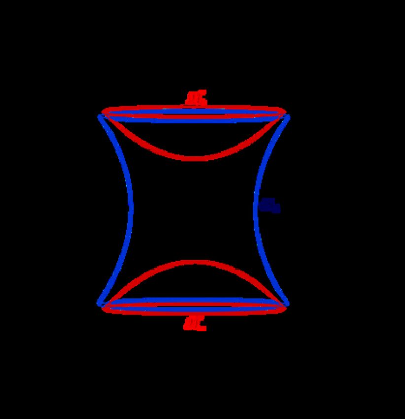
–6–Figure 2. The wedge holography setup. Here Σ → − 0 is implemented through introducing a large
JHEP01(2023)138
cutoff surface v∞ near the boundary and then taking v∞ →− ∞.
3.1 Wedge holography: a brief review
Wedge holography [13, 28] is a realisation of co-dimension two holography where the dual
theory of a (d+1) dimensional gravity theory lives in some (d-1) dimensional surface rather
than the usual d-dimensional one. It was proposed as a generalisation of AdS/CFT and
then later was used4 in understanding Celestial holography in flat spacetime [31].
The basic idea is to consider a “wedge” region W in a (d+1) dimensional bulk spacetime
M bounded by two EoW branes Q1 and Q2 . The part of the boundary ∂M of the full
manifold within W , is denoted as Σ. The classical gravity in the wedge region is defined by
specifying Neumann boundary conditions on Q1 and Q2 while the usual Dirichlet boundary
conditions are imposed on Σ. Then the proposal of Wedge Holography states [13]:
Classical gravity on the Wedge region is dual to a CFT living on Σ in the limit
when the width of Σ is going to zero.
In the above limit the surface Σ becomes a (d-1) dimensional surface in which the CFT
lives. Thus we have a co-dimension two holography. In case of flat space, the wedge region
is selected in the Milne region and in the Rindler region separately [31]. In Milne patch,
the wedge region is bounded by two AdS2 slices with proper distance τ1 and τ2 from the
origin O. Similarly, in Rindler patch, the wedge region is bounded by dS 2 slices at proper
distance ξ1 and ξ2 . In both cases, the (d-1) surface is then the u = 0 surface at null infinity.
We employ wedge holography in these two regions separately and then match the
boundary conditions on u = 0. First, we keep the boundaries of the wedge region to be
fixed and then allow fluctuating boundaries. In later case we get an effective JT theory on
the EoW branes.
3.2 Reduction to rigid slices
As stated above, we consider a region W within the Milne patch bounded by two AdS2
slices at τ = τ1 and τ = τ2 . The 3D gravity action supplemented by appropriate boundary
4
Wedge holography has also been used in [29, 30] in understanding concepts related to black hole
information paradox.
–7–terms with Neumann boundary condition is as follows,
1
Z Z q
= d x̂ −ĝ R̂ + 2
3
d x̂ ĥ(1) (K̂ (1) − T (1) )
2
p
SW
16πGN W Q1
Z q
−2 d2 x̂ ĥ(2) (K̂ (2) − T (2) ) . (3.2)
Q2
(i)
Here Qi is the boundary at τ = τi , with induced metric ĥ(i) , outgoing unit normal n̂A ,
trace of extrinsic curvature K̂ (i) , and “tension” T (i) .5 Variation of the action SW gives,
R̂
JHEP01(2023)138
R̂AB − ĝAB = 0, (3.3)
2
as expected. The Neumann boundary condition on Qi is given as,
(i) (i)
K̂AB = (K̂ (i) − T (i) )ĥAB . (3.4)
For the bulk metric (2.16), the outgoing normal at Q(i) is simply,
(i)
n̂A = (−1, 0, 0),
and the extrinsic curvature of the surface can be calculated to be,
2
K̂ (i) = .
τi
Thus from Israel Junction condition, the tension on the slice is given by:
1
T (i) = . (3.5)
τi
The coordinates in W are denoted as x̂A ≡ {τ, xµ }, where xµ ≡ {ρ, θ} are the coordinates
on the AdS2 slices. Now we want to perform a consistent dimensional reduction to write
down a low energy effective action on the AdS2 slices. In principle, this requires us to vary
all components of the bulk metric around the vacuum solution. But since we are interested
only in the massless modes in the 2D effective theory, we can choose the following ansatz:
ds2 = −dτ 2 + τ 2 gµν (x)dxµ dxν . (3.6)
It was shown by [32–34] that the modes coming from the variation of cross-terms gτ µ
correspond to massive modes in the effective theory and hence can be neglected. The
massless mode coming from the fluctuation of the gτ τ component can be interpreted as the
fluctuation of the location of the branes. We will consider this in the next section.
For this ansatz, we have the following expressions,
1 √ 2
q
R̂(ĝ) = 2 (R(g) + 2), ĥ(i) = τi2 g, K̂ (i) = .
τ τi
5
There is no boundary term for Neumann boundary condition, that makes the variation of the action
zero on-shell. Hence, the “tension” is added to the boundary which corresponds to having some localized
matter on the boundary. Here it is taken to be constant for simplicity.
–8–Figure 3. The EoW brane and its fluctuations. (a) is a fixed AdS2 brane. (b) shows a rigid brane
with spatial fluctuations. (c) shows fluctuating brane configuration. The green circle denotes the
fixed metric at the boundary due to Dirichlet boundary condition.
JHEP01(2023)138
Using these relations in (3.2) and then performing the τ integral, we obtain the low energy
effective theory as follows,
τ2 − τ1 √
Z
Seff = d2 x gR. (3.7)
16πGN
This is nothing but the Einstein-Hilbert action in two dimensions, with an effective 2D
Newton constant given as,
GN
G2 ≡ . (3.8)
τ2 − τ1
The 2D effective action (3.7) we got is proportional to the Euler character of the manifold,
which is a topological invariant. It has no dynamics. This can also be understood from
the fact that the 2D Einstein tensor is trivially zero by construction. 6 Although in 3D, the
asymptotically flat spacetimes are solutions to the Einstein equation which in turn fixes
the metric on the 2D slices to be asymptotically AdS2 , we cannot get this condition by
simply varying the 2D pure gravity action. Thus as long as superrotation symmetry is
there (which is the case for rigid branes), we get no non-trivial dynamics.
To break this superrotation symmetry, we consider small fluctuations in the location
of the branes. As we see below, the fluctuations non-minimally couple to gravity in the
effective theory. We essentially use a similar technique to [16, 17], where brane fluctuations
were considered in AdS3 wedge holography. The authors show that these fluctuations are
important in the understanding of entanglement entropy. Brane fluctuations in AdS 3 and
its effects in entanglement entropy were also studied in [18].
3.3 Reduction to fluctuating AdS2 slices
We now consider small fluctuations in the location of the AdS2 hypersurfaces, and choose
the boundary conditions such that the tension of the branes are held fixed. 7 Again, in low
energy description, we consider this additional mode to be independent of τ . The location
of the boundary Qi of W is now given by,
τ = τi (1 + φi (x)). (3.9)
φi (x) are dimensionless fields that we consider to be very small and we will work up to
quadratic order in these fields. The bulk computation remains the same, where only the
6
This condition enforces any cosmological constant term to be zero in pure 2D gravity.
7
This fixes the cosmological constant on the AdS2 slices.
–9–τ -integration limits change. On the branes we have,
1
(i)
n̂A = 1 + (∇φi )2 (−1, τi ∇µ φi ),
2
2 1 2
K̂ (i) = + (∇2 φi − 2φi ) + (φ2i − φi ∇2 φi ),
τi τi τi
√ 1
p
h̃(i) = τi2 g 1 + 2φi + φ2i − (∇φi )2 .
2
We use these expressions in (3.2) and then perform the τ integral, to get the effective
JHEP01(2023)138
action up to quadratic order in φ,
τ2 − τ1 √ 1 √
Z Z
Seff = d2 x gR + d2 x g[(τ2 φ2 − τ1 φ1 )(R + 2) + 2(τ1 ∇2 φ1 − τ2 ∇2 φ2 )]
16πGN 16πGN
1 √
Z
+ d2 x g[τ2 (∇φ2 )2 + 2τ2 φ22 − τ1 (∇φ1 )2 − 2τ1 φ21 ]. (3.10)
16πGN
We already see a dilaton gravity theory as the low energy effective theory for the wedge.
3.3.1 Effective action for the whole hyperbolic patch
Finally we take the limits τ1 → 0 and τ2 = τ∞ for large τ∞ such that we cover the full
hyperbolic patch. Writing φ2 ≡ φ, the effective action is given by,
τ∞ √
Z
Seff = d2 x g[R + φ(R + 2) − 2∇2 φ + (∇φ)2 + 2φ2 ]. (3.11)
16πGN
We further perform a Weyl transformation of the metric g → e−φ g, such that the kinetic
and mass term of φ gets absorbed in the Ricci scalar,
τ∞ √
Z
Seff = d2 x g[R + φ(R + 2) + ∇µ (φ∇µ φ − ∇µ φ)]. (3.12)
16πGN
This is the bulk part of the JT action up to a total derivative term. In this action, we have
dynamical gravity. The dilaton and metric equations of motion are,
R + 2 = 0, (3.13)
∇µ ∇ν φ − gµν ∇ φ + gµν φ = 0.
2
(3.14)
Thus we see that the dilaton EOM fixes the scalar curvature of the 2D slices to -2. The
solutions are asymptotically AdS2 spacetimes. All these solutions are exact zero modes for
a constant dilaton profile. But the dilaton profile can in principle be non-trivial at the bulk
which makes these modes become slightly nondegenerate (up to the SL(2, R) isometry of
global AdS2 ) in presence of appropriate boundary term. In the 3D picture, it implies that a
wedge region with fluctuating boundary breaks the degeneracy between 3D asymptotically
flat spacetimes.
– 10 –3.3.2 Fall-off condition for the dilaton
As we just saw, the advent of the dilaton in the effective theory is due to fluctuations of
the branes that bound the wedge region. The asymptotic geometry of these branes is fixed
from asymptotic flatness condition of (2+1)D. But we still need to impose a non-trivial
boundary condition for the dilaton. As it has been extensively studied, the general fall-off
condition for the dilaton, consistent with the EOMs in 2D, is given by:
φ(ρ̃ → ∞, θ) = P (θ)eρ̃ + O(e−ρ̃ ). (3.15)
It has been discussed in [20] that through a redefinition of the boundary time coordinate,
JHEP01(2023)138
the θ dependence from the boundary value of the dilaton can be stripped off. Therefore at
leading order, we will consider the following asymptotic behavior of the dilaton,
ρ̃→∞
φ −−−→ φr eρ̃ , (3.16)
where, φr is a constant. This boundary condition is important for getting a non-trivial
dynamics at the boundary.
3.4 Fluctuating dS2 patch: analytic continuation
The effective action on the Rindler wedge, which is bounded by two Lorentzian dS 2 branes
can be calculated quite similarly. The fields on dS2 brane are analytic continuations from
the EAdS slice. Along with the continuation of coordinates (2.6), we now have the following
identifications:
LAdS → −iLdS , φ → ψ, (3.17)
where L(A)dS is the radius of the (A)dS brane and ψ is the scalar mode for fluctuations in
the location of the dS2 slice. Thus the effective action on the dS2 brane can be written as,
ξ∞ √
Z
Seff ∼ d2 x −g[R + ψ(R − 2)]. (3.18)
16πGN
Here once again we have chosen the limits of the wedge region to cover the whole Rindler
patch. Similar to (3.12), this action also has an inconsequential total derivative term with it.
The analytic continuation also helps fix the boundary behaviour of the metric and dila-
ton field. Although, dS2 have two conformal boundaries, in [35] it was shown that specifying
the boundary conditions in either one is sufficient since they are anti-podally identified.
Since we are interested in the behaviour near future null infinity in 3D, we will study the
boundary behaviour of dS2 fields near future conformal boundary. The conditions are,
1 2η̃ M
2 η̃→∞
ds −−−→ −dη̃ + 2
e + + . . . dθ2 , (3.19)
4 2
η̃→∞
ψ −−−→ iφr eη̃ . (3.20)
√
The coordinate η̃ is given as η̃ ≡ η + ln M , where η is defined through (2.6). As we see
below these boundary behavior crucially fixes the effective dynamics.
– 11 –4 Boundary Schwarzian theory
Now that we have understood the effective action on the hyperbolic/dS2 slices, we begin
to formulate 1D dual theory as advertised earlier. Both the 3D pure gravity theory and 2D
JT gravity are topological theories, hence their dynamics crucially depends on boundary
degrees of freedom. In this section, we carefully calculate the boundary action on u = 0
slice of null infinity.
4.1 Null boundary term for 3D gravity
In general for Einstein-Hilbert action, we need to add a boundary term for a well defined
JHEP01(2023)138
variational principle. In a region with spacelike or timelike boundary, one usually adds a
Gibbons-Hawking-York term but in our case the boundary is null. So the usual prescription
fails. Ref. [36] has a relatively recent proposal for a counter term to be added at null
boundaries. We briefly sketch the construction without proof and use it to calculate the
necessary boundary term for us.
4.1.1 General construction
For a codimension-1 null hypersurface defined by ϕ(x) = 0, the null vector lA ≡ λ(x)∂A ϕ
is normal to the surface. Unlike non-null hypersurfaces, there is no notion of a unit normal
since its norm is zero. The usual projector, orthogonal to the normal direction, also does
not work since the induced metric on the codimension-1 hypersurface is degenerate.
The vector lA is also tangent to the null hypersurface and thus we can define integral
A
curves along the surface corresponding to lA given by dx dα = l . Along these curves, θ
A
is constant. Thus α parameterises the null geodesics and θ represents the coordinates on
the spatial slice of the null hypersurface. The hypersurface can be covered by coordinates
{α, θ}. Depending on the parameterisation α, the null geodesics described above satisfy
lA ∇A lB = κlB , where κ is the inaffinity.
It is possible to define a nondegenerate induced metric on this spatial slice, which
in case of 3D is just one dimensional. To do so, a linearly independent basis should be
constructed, given by {lA , k A , EθA } such that,
∂xA
lA lA = kA k A = 0; lA k A = −1; EθA = ; lA EθA = kA EθA = 0. (4.1)
∂θ
Here k A is an auxiliary null vector. Now the induced metric on the spatial slice can be
defined as,
qAB = gAB + lA kB + kA lB . (4.2)
A acts as a projector on the spatial slice, orthogonal to both lA and k A . Equipped with
qB
this, [36] constructed a boundary term that is suitable to make the variation of the Einstein-
Hilbert action well-defined on a manifold with null boundary. We are imposing Dirichlet
boundary condition on the metric. Then the boundary action is given by,
1 √
Z
Sbdy = dαdθ q(Θ + κ). (4.3)
8πGN
Here Θ = g CD qC D C D is called the expansion scalar and q is the determinant of the
AqB ∇ l
metric qAB , projected on the spatial slice.
– 12 –4.1.2 Null boundary term from 3D asymptotically flat spaces
Now we want to compute the contribution coming from the null boundary term in the wedge
region W , bounded by hyperbolic slices. The location of the EoW branes dictate the inte-
gration range for the null geodesic parameter. We go to a double null coordinates (u, v, θ)
from (u, r, θ) using r = 12 (v − M u) such that the metric (2.9) for J = 0 takes the form,
1
ds2 = −dudv + (v − M u)2 dθ2 . (4.4)
4
The null boundary I + is located at v = v∞ such that v∞ → ∞. Normal to this boundary
JHEP01(2023)138
lA = λ∂A (v − v∞ ) = λ(0, 1, 0), lA = (−2λ, 0, 0). (4.5)
We have put an arbitrary constant λ in front of the normal since the normalization cannot
be fixed. The coordinates adapted to the null geodesics on I + is given as (u, θ) such that,
dxA
∝ lA . (4.6)
du
The null geodesics are affinely parametrized w.r.t. u since lA ∇A lB = 0 i.e. the inaffinity
parameter κ = 0. The auxilliary null vector for this surface is then given by,
∂xA
k A kA = 0, k A lA = −1, kA = 0,
∂θ (4.7)
1 1
=⇒ kA = , 0, 0 , k A = 0, − , 0 .
2λ λ
Now we have the necessary quantities to calculate the induced metric on the spatial slice.
Using (4.2) we get,
1 √ 1
qAB = gAB + lA kB + kA lB = diag 0, 0, (v − M u)2 ; q = (v − M u). (4.8)
4 2
We can also calculate the expansion scalar to be,
2λM
Θ= . (4.9)
v − Mu
As discussed above, the boundary term to be added to (3.1) for a well-defined variational
principle with Dirichlet boundary condition is given by,
1
Z u2
√ λ λ
Z Z Z
Sbdy = dudθ q(Θ + κ) = dθM du = dθM (u2 − u1 ),
8πGN 8πGN u1 8πGN
(4.10)
where the limits of the u-integration are determined by the cut-off on the fluctuating EoW
branes. We introduce this cutoff via (large) constant v surfaces. In hyperbolic coordinates
these are given by,
v = M u + 2r = τ eρ̃ = v∞ , (4.11)
– 13 –where the boundary I + is given by v∞ → ∞. This cutoff inherits a cutoff along the radial
direction for the fluctuating AdS2 branes. For the brane given by τ = τi (1 + φi ) the radial
cutoff is at ρ̃i such that,
τi (1 + φi )eρ̃i = v∞ . (4.12)
Then from the coordinate transformation relations we have,
ui = τi (1 + φi )e−ρ̃i , (4.13)
as the limits of the above integral. The null boundary term (4.10) becomes,
λ
JHEP01(2023)138
Z
Sbdy = dθM τ2 e−ρ̃2 − τ1 e−ρ̃1 + τ2 φ2 e−ρ̃2 − τ1 φ1 e−ρ̃1 . (4.14)
8πGN
We take the limits τ2 = τ∞ and τ1 → 0 and we rewrite φ2 = φ and ρ̃2 = ρ̃∞ . For the
boundary behavior of the dilaton (3.16),
φ = φr eρ̃∞ , (4.15)
the null boundary term (4.10) is given as under the limit ρ̃∞ → ∞,
λ
Z
Sbdy = τ∞ dθφr M. (4.16)
8πGN
Now we show that this term exactly matches with the boundary term from 2D effective
theory.
4.2 GHY term for 2D (A)dS2 slices
From (2.16) we have that on a constant τ = τi slice, the asymptotically AdS2 metric has
the following form,
1 2ρ̃ M
ds2 = dρ̃2 + e − + O e−2ρ̃ dθ2 . (4.17)
4 2
The boundary of this asymptotically AdS2 spacetime is given by the intersection of the
constant τ slice and the v = v∞ surface. Therefore it is located at a constant radial
distance ρ̃ = ρ̃i given by (4.12) with Dirichlet boundary condition on the metric. For
the metric (4.17), we can construct the unit normal nµ , induced metric γµν , and extrinsic
curvature K as,
nµ = (1, 0),
√ 1 2ρ̃ M 1/2
γ= e − ,
4 2
e2ρ̃
K = 2ρ̃ ,
e − 2M
√ 1 M −ρ̃
γK = eρ̃ + e + O e−2ρ̃ .
2 2
Using the falloff (3.16) of the dilaton, we have
√ φr
Z Z
dx γφ(K − 1) = dθM (θ). (4.18)
2
– 14 –Using this condition, the null boundary term of 3D gravity in the hyperbolic region with
asymptotic flat boundary conditions, reduces to the GHY boundary term required for the
2D action (3.12),
τ∞ √ τ∞ φ r
Z Z
IMilne = γφ(K − 1) = dθM (θ). (4.19)
8πGN 16πGN
We have made the choice λ = 12 , which was arbitrary.
The GHY term required for the effective action (3.18) in Rindler region, can be simi-
larly computed from the null boundary term,
JHEP01(2023)138
ξ∞ √ iξ∞ φr
Z Z
IRindler =− γψ(K − 1) = − dθM (θ). (4.20)
8πGN 16πGN
Using ξ∞ = iτ∞ , we find that this contribution is exactly equal to the boundary term (4.19)
and they add up at u = 0.
4.3 1D effective action: Schwarzian
The effective theory that describes the dynamics of 3D asymptotically flat spacetimes
(which are related to the flat spacetime through superrotations) in the hyperbolic region,
is given by (3.12) along with the boundary contribution (4.19),
1 √
Z
Seff = d2 x gR + SJT . (4.21)
16πG2
G2 = G τ∞ is the effective two-dimensional Newton constant. In Kaluza-Klein reduction
N
also, the effective lower dimensional coupling constant is given by a combination of the
volume of the compact manifold and the higher dimensional coupling. In our non-compact
reduction, we have regulated the “infinite box” to a finite size through the introduction
of a large cutoff τ∞ . Similar to Kaluza-Klein reduction, the effective coupling depends on
this cutoff i.e. the size of the “finite box”.
The first term in the action is a constant and the second term in the JT action given as,
1 √ √
Z Z
SJT = d2 x gφ(R + 2) + 2 dx γφ(K − 1) . (4.22)
16πG2
We have dropped off the total derivative piece from (3.12) since its variation is zero in the
boundary with our boundary conditions. Hence this term does not affect the dynamics of
the system.
In the JT action (4.22), the dilaton φ is a Lagrange multiplier, hence it can be simply
integrated out by plugging the dilaton equation of motion into the action, which sets
R + 2 = 0 [20]. This corresponds to asymptotically AdS2 geometries and gives an effective
one-dimensional Schwarzian theory coming from the boundary term (4.19). As expected,
this is consistent with the asymptotic AdS2 boundary conditions that we have obtained
from the superrotated 3D spacetimes.
The boundary theory describes the dynamics of the boundary graviton in 2D, which we
have identified to be coming from the superrotation mode of 3D gravity. We have already
– 15 –seen that the function M (θ) transforms as an infinitesimal Schwarzian derivative under the
action of 3D superrotation generators. From the 2D perspective [27], it was shown that the
O(1) correction appearing in (4.17), transforms as an infinitesimal Schwarzian derivative
under the action of the asymptotic Killing vectors of AdS2 .
An exact replica of this calculation would occur for dS2 slices. After integrating out
ψ from the effective action (3.18) we get R − 2 = 0 [37, 38]. In this case also, the theory
reduces to a similar 1D boundary theory as in (4.20). Thus the effective action (considering
contributions from both Milne and Rindler patches) at the u = 0 circle that describes the
low energy dynamics of 3D asymptotically flat spaces is given by,
JHEP01(2023)138
φr
Z
S1D = IMilne + IRindler = dθM (θ). (4.23)
8πG2
Due to time translation symmetry in 3D, this effective theory may live on any spatial slice of
I + . For superrotated spacetimes in 3D, this action can be thought of as the (nearly) Celes-
tial CFT dual of the 3D pure gravity theory. This effective action (4.23) is closely related to
the action of superrotation Goldstone modes derived in [21] through a different prescription.
An exactly similar effective action can be written down at v = 0 surface of past
null infinity I− . There the Schwarzian theory would be described in terms of M̃ , the
superrotation modes at I− . But this is not an independent theory as M̃ is related to
M (θ) via antipodal matching condition. Hence the 1D theory can be described either at
I+ or I− . In the dimensionally reduced picture this implies that the hyperbolic slices
on H+ and H− have boundary conditions that are antipodally matched. For dS2 slices,
antipodal matching of 3D implies the boundary conditions on future and past conformal
boundary to be identified (as expected in [35]).
5 Conclusions and outlook
In this paper we study the low energy effective dynamics of pure gravity in asymptotically
flat spacetime. We start by reducing the 3D theory on a wedge region bounded by two
asymptotically (A)dS2 slices in Milne and Rindler patches separately. Finally we take the
limit when the wedge regions cover the full spacetime. The localised action at these slices
turn out to be JT gravity when fluctuations of the EoW branes are taken into account.
Using the dual boundary description of JT gravity, we find that the co-dimension two holo-
graphic dual is a Schwarzian theory that lives at a spatial slice of I + . The superrotation
mode in 3D acts as the Schwarzian in this action. In this process, we identify that the
Virasoro subalgebra of BMS3 , generated by the superrotations, maps to the asymptotic
symmetry algebra of (A)dS2 . Evidently, this is nothing but the local conformal algebra
(or diffeomorphisms) of the 1D boundary. This is an explicit construction of a Celestial
(nearly) CFT in low energy limit.
The φ mode we have introduced to break superrotation symmetry needs to be un-
derstood more. It clearly has non-trivial boundary value and hence behaves as a large
diffeomorphism. The equation of motion (3.14) suggests that φ can be interpreted as a
large diffeomorphism in harmonic gauge. We hope to explore this further in a future work.
– 16 –There are several directions to explore from here. Firstly, we only considered super-
rotated spacetimes in 3D as those solutions respect the hyperbolic foliation crucial for the
construction. The effect of 3D supertranslations on this effective theory needs to be under-
stood and we want to explore this further. Understanding the 1D dual theory in presence
of fermionic symmetries of (2+1)D supergravity theories [39–43] would be interesting. The
1D dual picture we have, also must relate to the 2D Wess-Zumino-Witten/Liouville dual
description of 3D gravity (See [44] for pure gravity and [39, 41, 45] for supergravity). The
relation between Lioville theories and Schwarzian are studied in [46, 47]. Also, the explicit
relations between correlators in 3D flat space and the ones coming from the Schwarzian
action needs to be understood further.
JHEP01(2023)138
In [48] the one loop partition function for 3D flat space was calculated, shown to
be related to the characters of the BMS3 group. It would be interesting to understand
this partition function from the 1D effective theory point of view. It has been shown
that JT gravity is dual to a random matrix model [49]. It is worth exploring if there
is some correspondence between 3D gravity with matrix models, via its duality with the
Schwarzian. Supertranslations may non-trivially affect this description. Along this line,
we would also like to understand whether there is a connection with the construction of
BMS3 invariant matrix models [50].
Acknowledgments
We are grateful to Nabamita Banerjee, Dileep Jatkar, Alok Laddha and Tadashi Takayanagi
for illuminating discussions and useful comments on the draft. MS would like to thank
Tabasum Rahnuma for helpful discussions. We would like to thank the people of India for
their continuous support towards research in basic sciences.
Open Access. This article is distributed under the terms of the Creative Commons
Attribution License (CC-BY 4.0), which permits any use, distribution and reproduction in
any medium, provided the original author(s) and source are credited. SCOAP 3 supports
the goals of the International Year of Basic Sciences for Sustainable Development.
References
[1] A. Strominger, Lectures on the infrared structure of gravity and gauge theory,
arXiv:1703.05448 [INSPIRE].
[2] S. Pasterski, S.-H. Shao and A. Strominger, Flat space amplitudes and conformal symmetry
of the celestial sphere, Phys. Rev. D 96 (2017) 065026 [arXiv:1701.00049] [INSPIRE].
[3] A. Laddha, S.G. Prabhu, S. Raju and P. Shrivastava, The holographic nature of null infinity,
SciPost Phys. 10 (2021) 041 [arXiv:2002.02448] [INSPIRE].
[4] D. Kapec, P. Mitra, A.-M. Raclariu and A. Strominger, 2D stress tensor for 4D gravity,
Phys. Rev. Lett. 119 (2017) 121601 [arXiv:1609.00282] [INSPIRE].
[5] G. Barnich and C. Troessaert, Symmetries of asymptotically flat 4 dimensional spacetimes at
null infinity revisited, Phys. Rev. Lett. 105 (2010) 111103 [arXiv:0909.2617] [INSPIRE].
– 17 –[6] S. Pasterski and S.-H. Shao, Conformal basis for flat space amplitudes, Phys. Rev. D 96
(2017) 065022 [arXiv:1705.01027] [INSPIRE].
[7] G. Barnich and C. Troessaert, Supertranslations call for superrotations, PoS CNCFG2010
(2010) 010 [arXiv:1102.4632] [INSPIRE].
[8] M. Campiglia and A. Laddha, Asymptotic symmetries and subleading soft graviton theorem,
Phys. Rev. D 90 (2014) 124028 [arXiv:1408.2228] [INSPIRE].
[9] D. Kapec, V. Lysov, S. Pasterski and A. Strominger, Semiclassical Virasoro symmetry of the
quantum gravity S-matrix, JHEP 08 (2014) 058 [arXiv:1406.3312] [INSPIRE].
[10] G. Barnich and C. Troessaert, Aspects of the BMS/CFT correspondence, JHEP 05 (2010)
JHEP01(2023)138
062 [arXiv:1001.1541] [INSPIRE].
[11] J. de Boer and S.N. Solodukhin, A holographic reduction of Minkowski space-time, Nucl.
Phys. B 665 (2003) 545 [hep-th/0303006] [INSPIRE].
[12] C. Cheung, A. de la Fuente and R. Sundrum, 4D scattering amplitudes and asymptotic
symmetries from 2D CFT, JHEP 01 (2017) 112 [arXiv:1609.00732] [INSPIRE].
[13] I. Akal, Y. Kusuki, T. Takayanagi and Z. Wei, Codimension two holography for wedges,
Phys. Rev. D 102 (2020) 126007 [arXiv:2007.06800] [INSPIRE].
[14] R. Jackiw, Lower dimensional gravity, Nucl. Phys. B 252 (1985) 343 [INSPIRE].
[15] C. Teitelboim, Gravitation and Hamiltonian structure in two space-time dimensions, Phys.
Lett. B 126 (1983) 41 [INSPIRE].
[16] H. Geng et al., Jackiw-Teitelboim gravity from the Karch-Randall braneworld, Phys. Rev.
Lett. 129 (2022) 231601 [arXiv:2206.04695] [INSPIRE].
[17] H. Geng, Aspects of AdS2 quantum gravity and the Karch-Randall braneworld, JHEP 09
(2022) 024 [arXiv:2206.11277] [INSPIRE].
[18] F. Deng, Y.-S. An and Y. Zhou, JT gravity from partial reduction and defect extremal
surface, arXiv:2206.09609 [INSPIRE].
[19] J.M. Maldacena, J. Michelson and A. Strominger, Anti-de Sitter fragmentation, JHEP 02
(1999) 011 [hep-th/9812073] [INSPIRE].
[20] J. Maldacena, D. Stanford and Z. Yang, Conformal symmetry and its breaking in two
dimensional nearly anti-de-Sitter space, PTEP 2016 (2016) 12C104 [arXiv:1606.01857]
[INSPIRE].
[21] S. Carlip, The dynamics of supertranslations and superrotations in 2 + 1 dimensions, Class.
Quant. Grav. 35 (2018) 014001 [arXiv:1608.05088] [INSPIRE].
[22] H. Bondi, M.G.J. van der Burg and A.W.K. Metzner, Gravitational waves in general
relativity. 7. Waves from axisymmetric isolated systems, Proc. Roy. Soc. Lond. A 269 (1962)
21 [INSPIRE].
[23] R.K. Sachs, Gravitational waves in general relativity. 8. Waves in asymptotically flat
space-times, Proc. Roy. Soc. Lond. A 270 (1962) 103 [INSPIRE].
[24] M. Campiglia and A. Laddha, New symmetries for the gravitational S-matrix, JHEP 04
(2015) 076 [arXiv:1502.02318] [INSPIRE].
[25] A. Strominger, On BMS invariance of gravitational scattering, JHEP 07 (2014) 152
[arXiv:1312.2229] [INSPIRE].
– 18 –[26] G. Barnich and H.A. Gonzalez, Dual dynamics of three dimensional asymptotically flat
Einstein gravity at null infinity, JHEP 05 (2013) 016 [arXiv:1303.1075] [INSPIRE].
[27] D. Grumiller, R. McNees, J. Salzer, C. Valcárcel and D. Vassilevich, Menagerie of AdS2
boundary conditions, JHEP 10 (2017) 203 [arXiv:1708.08471] [INSPIRE].
[28] R.-X. Miao, An exact construction of codimension two holography, JHEP 01 (2021) 150
[arXiv:2009.06263] [INSPIRE].
[29] H. Geng et al., Information transfer with a gravitating bath, SciPost Phys. 10 (2021) 103
[arXiv:2012.04671] [INSPIRE].
[30] H. Geng, S. Lüst, R.K. Mishra and D. Wakeham, Holographic BCFTs and communicating
JHEP01(2023)138
black holes, JHEP 08 (2021) 003 [arXiv:2104.07039] [INSPIRE].
[31] N. Ogawa, T. Takayanagi, T. Tsuda and T. Waki, Wedge holography in flat space and
celestial holography, Phys. Rev. D 107 (2023) 026001 [arXiv:2207.06735] [INSPIRE].
[32] L. Randall and R. Sundrum, An alternative to compactification, Phys. Rev. Lett. 83 (1999)
4690 [hep-th/9906064] [INSPIRE].
[33] L. Randall and R. Sundrum, A large mass hierarchy from a small extra dimension, Phys.
Rev. Lett. 83 (1999) 3370 [hep-ph/9905221] [INSPIRE].
[34] A. Karch and L. Randall, Locally localized gravity, JHEP 05 (2001) 008 [hep-th/0011156]
[INSPIRE].
[35] A. Strominger, The dS/CFT correspondence, JHEP 10 (2001) 034 [hep-th/0106113]
[INSPIRE].
[36] K. Parattu, S. Chakraborty, B.R. Majhi and T. Padmanabhan, A boundary term for the
gravitational action with null boundaries, Gen. Rel. Grav. 48 (2016) 94 [arXiv:1501.01053]
[INSPIRE].
[37] J. Cotler, K. Jensen and A. Maloney, Low-dimensional de Sitter quantum gravity, JHEP 06
(2020) 048 [arXiv:1905.03780] [INSPIRE].
[38] J. Maldacena, G.J. Turiaci and Z. Yang, Two dimensional nearly de Sitter gravity, JHEP 01
(2021) 139 [arXiv:1904.01911] [INSPIRE].
[39] G. Barnich, L. Donnay, J. Matulich and R. Troncoso, Super-BMS3 invariant boundary theory
from three-dimensional flat supergravity, JHEP 01 (2017) 029 [arXiv:1510.08824]
[INSPIRE].
[40] O. Fuentealba, J. Matulich and R. Troncoso, Asymptotic structure of N = 2 supergravity in
3D: extended super-BMS3 and nonlinear energy bounds, JHEP 09 (2017) 030
[arXiv:1706.07542] [INSPIRE].
[41] N. Banerjee, A. Bhattacharjee, Neetu and T. Neogi, New N = 2 super-BMS3 algebra and
invariant dual theory for 3D supergravity, JHEP 11 (2019) 122 [arXiv:1905.10239]
[INSPIRE].
[42] I. Lodato and W. Merbis, Super-BMS3 algebras from N = 2 flat supergravities, JHEP 11
(2016) 150 [arXiv:1610.07506] [INSPIRE].
[43] N. Banerjee, I. Lodato and T. Neogi, N = 4 supersymmetric BMS3 algebras from asymptotic
symmetry analysis, Phys. Rev. D 96 (2017) 066029 [arXiv:1706.02922] [INSPIRE].
– 19 –[44] G. Barnich, A. Gomberoff and H.A. González, Three-dimensional Bondi-Metzner-Sachs
invariant two-dimensional field theories as the flat limit of Liouville theory, Phys. Rev. D 87
(2013) 124032 [arXiv:1210.0731] [INSPIRE].
[45] N. Banerjee, A. Bhattacharjee, S. Biswas and T. Neogi, Dual theory for maximally N
extended flat supergravity, JHEP 05 (2022) 179 [arXiv:2110.05919] [INSPIRE].
[46] T.G. Mertens, G.J. Turiaci and H.L. Verlinde, Solving the Schwarzian via the conformal
bootstrap, JHEP 08 (2017) 136 [arXiv:1705.08408] [INSPIRE].
[47] T.G. Mertens, The Schwarzian theory — origins, JHEP 05 (2018) 036 [arXiv:1801.09605]
[INSPIRE].
JHEP01(2023)138
[48] G. Barnich, H.A. Gonzalez, A. Maloney and B. Oblak, One-loop partition function of
three-dimensional flat gravity, JHEP 04 (2015) 178 [arXiv:1502.06185] [INSPIRE].
[49] P. Saad, S.H. Shenker and D. Stanford, JT gravity as a matrix integral, arXiv:1903.11115
[INSPIRE].
[50] A. Bhattacharjee and Neetu, Matrix model with 3D BMS constraints, Phys. Rev. D 105
(2022) 066012 [arXiv:2108.07314] [INSPIRE].
– 20 –You can also read