Inspecting class hierarchies in classification-based metric learning models
←
→
Page content transcription
If your browser does not render page correctly, please read the page content below
Inspecting class hierarchies in classification-based metric
                                                       learning models
                                                       Hyeongji Kim1,2* , Pekka Parviainen2 , Terje Berge1 , Ketil Malde1,2

                                                       1 Institute of Marine Research, Bergen, Norway
                                                       2 Department of Informatics, University of Bergen, Norway

                                                       * hjk92g@gmail.com
arXiv:2301.11065v1 [cs.LG] 26 Jan 2023

                                                       Abstract
                                                       Most classification models treat all misclassifications equally. However, different classes
                                                       may be related, and these hierarchical relationships must be considered in some
                                                       classification problems. These problems can be addressed by using hierarchical
                                                       information during training. Unfortunately, this information is not available for all
                                                       datasets. Many classification-based metric learning methods use class representatives in
                                                       embedding space to represent different classes. The relationships among the learned
                                                       class representatives can then be used to estimate class hierarchical structures. If we
                                                       have a predefined class hierarchy, the learned class representatives can be assessed to
                                                       determine whether the metric learning model learned semantic distances that match our
                                                       prior knowledge. In this work, we train a softmax classifier and three metric learning
                                                       models with several training options on benchmark and real-world datasets. In addition
                                                       to the standard classification accuracy, we evaluate the hierarchical inference
                                                       performance by inspecting learned class representatives and the hierarchy-informed
                                                       performance, i.e., the classification performance, and the metric learning performance
                                                       by considering predefined hierarchical structures. Furthermore, we investigate how the
                                                       considered measures are affected by various models and training options. When our
                                                       proposed ProxyDR model is trained without using predefined hierarchical structures,
                                                       the hierarchical inference performance is significantly better than that of the popular
                                                       NormFace model. Additionally, our model enhances some hierarchy-informed
                                                       performance measures under the same training options. We also found that
                                                       convolutional neural networks (CNNs) with random weights correspond to the
                                                       predefined hierarchies better than random chance.

                                                       Introduction
                                                       Neural network-based classifiers have shown impressive classification accuracy. For
                                                       instance, a convolutional neural network (CNN) classifier [1] surpassed human-level
                                                       top-5 classification accuracy (94.9%) [2] on the 1000-class classification challenge on the
                                                       ImageNet dataset [3]. Most training loss functions in neural network classifiers treat all
                                                       misclassifications equally. However, in practice, the severity of various misclassifications
                                                       may differ considerably. For instance, in an autonomous vehicle system, mistaking a
                                                       person as a tree can result in a more catastrophic consequence than mistaking a
                                                       streetlight as a tree [4]. In addition, some classification tasks include a large number of
                                                       classes, such as the 1000-class ImageNet classification challenge, and hierarchical
                                                       relationships may exist among these classes. When several classification models

                                    January 27, 2023                                                                                          1/49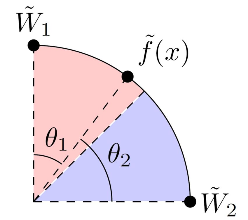
achieved similar accuracy, one would prefer to choose models in which the wrongly
                   predicted classes are “hierarchically” close to the ground-truth classes. To address the
                   severity of misclassifications and relationships among classes, hierarchical information
                   can be used. For instance, predefined hierarchical structures can be incorporated into
                   training by replacing standard labels with soft labels based on this hierarchical
                   information [4]. Some metric learning approaches also use hierarchical information [5–7].
                       In general, metric learning methods learn embedding functions in which similar data
                   points are close and dissimilar data points are far apart according to the distance metric
                   in the learned embedding space. For class-labeled datasets, data points in the same
                   class are regarded as similar, while data points in different classes are regarded as
                   dissimilar. Metric learning can be applied in image retrieval tasks [8] to identify relevant
                   images or few-shot classification tasks [9, 10], which are classification tasks with only a
                   few examples per class. Usually, metric learning methods assume that there are no
                   special relations among classes, i.e., a flat hierarchy is assumed. However, a predefined
                   class hierarchy can be incorporated into the training process of metric learning models
                   to improve the hierarchy-informed performance [5–7].
                       Class hierarchical structures can be defined in several ways. Hierarchical structures
                   can be defined by domain experts [6] or extracted from WordNet [11], which is a
                   database that contains semantic relations among English words. For instance, ImageNet
                   classes [3] are organized according to WordNet. However, hierarchy determination from
                   WordNet requires that a class name or its higher class is in the WordNet database.
                   When these approaches are not applicable, hierarchy can be inferred by estimating the
                   class distance matrix based on learned classifiers. For instance, the confusion matrix of
                   a classifier can be used to estimate relations among class pairs [12]. Each row in the
                   confusion matrix can be treated as a vector, and the distance between these vectors can
                   be calculated to estimate the class hierarchical structure. However, this approach can
                   be cumbersome for hierarchy-informed classification tasks, as they require separate
                   training and evaluation (validation) processes to determine the hierarchical structure.
                   Moreover, this approach becomes challenging when some classes contain a very small
                   number of data points, as some elements in the confusion matrix may be uninformative.
                   One type of metric learning model uses a unique position in embedding space (class
                   representative) to represent each class [13–16]. Class representatives can also be used to
                   infer hierarchical structures by considering their distances [6, 17]. This approach does
                   not require a separate training process, as class representatives can be learned
                   automatically.
                       On the other hand, when we have a predefined hierarchy, the learned class
                   representatives can improve our understanding of the trained metric learning model.
                   For example, we can determine if the semantic distance learned by a metric learning
                   model matches our prior knowledge (that is, the predefined hierarchy). For instance,
                   when a model has been trained to classify species, we can determine if the model
                   regards a dog as closer to a cat than to a rose. Furthermore, these inspections can be
                   used to evaluate the trustworthiness of a model. However, previous works have paid
                   little attention to the relationships among class representatives. In this work, we assess
                   several metric learning methods and training options by focusing on their learned class
                   representatives and hierarchy-informed performance. Moreover, we attempt to
                   determine conditions that improve the hierarchy inference performance and evaluate
                   whether such models enhance the hierarchy-informed performance. We also investigate
                   different training options with predefined hierarchies for comparison.

                   Problem settings
                   The predefined hierarchical distance, i.e., the distance between two classes, often needs
                   to be considered when training models with hierarchical information and evaluating

January 27, 2023                                                                                         2/49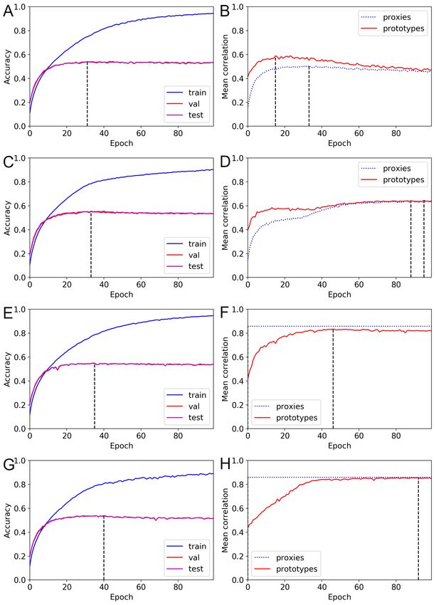
model performance. Barz and Denzler [5] and Bertinetto et al. [4] used bounded ([0, 1])
                   dissimilarity based on the height of the lowest common ancestor (LCA) between two
                   classes. In this work, similar to Garnot and Landrieu [6], we define the hierarchical
                   distance as the shortest path distance between two classes. For instance, in the
                   predefined hierarchical tree shown in Fig. 1, the hierarchical distance between the
                   classes “tiger” and “woman” is 4 (= 2 + 2), as we need to move two steps upward and
                   two steps downward to move from one class to the other. Similarly, the hierarchical
                   distance between the classes “tiger” and “shark” is 6. Hierarchical structures can be
                   expressed as trees or directed acyclic graph (DAG) structures [18]. In this work, we
                   consider tree-structured hierarchies. In other words, each node cannot have more than
                   one parent node.

                   Fig 1. Pruned CIFAR100 tree structure for visualization. The whole
                   hierarchical structure is shown in a table in S2 Appendix.

                      Let X ⊆ RdI be an input space and Y be a set of classes. The data points x ∈ X
                   and corresponding classes c ∈ Y are sampled from the joint distribution D. The feature
                   mapping f : X → Z extracts feature vectors according to the inputs, where Z = RdF is
                   a raw feature space. In this work, we assume that this mapping is modeled by a neural
                   network.

                   Softmax classification
                   The softmax classifier is commonly used in neural network-based classification tasks.
                   The softmax classifier estimates the class probability p(c|x), which is the probability
                   that data point x belongs to class c, as follows:

                                                             exp(lc (x))
                                                   p(c|x) = P              ,                             (1)
                                                               exp(ly (x))
                                                             y∈Y

                   where logit ly (x) is the neural network output according to input x ∈ X and class y ∈ Y.
                   Usually, logit ly (x) is calculated as:

                                                    ly (x) = WyT f (x) + by ,                            (2)

                   where the feature vector f (x) is an output of a penultimate layer, Wy is a weight vector,
                   and by is a bias term for class y. The probability p(c|x) estimated by the model is often
                   called the confidence value (score). Based on the estimated class probabilities, we can
                   use the cross-entropy loss to train the model. This loss measures the difference between
                   the predicted and target probability distributions. The cross-entropy (CE) loss of a

January 27, 2023                                                                                       3/49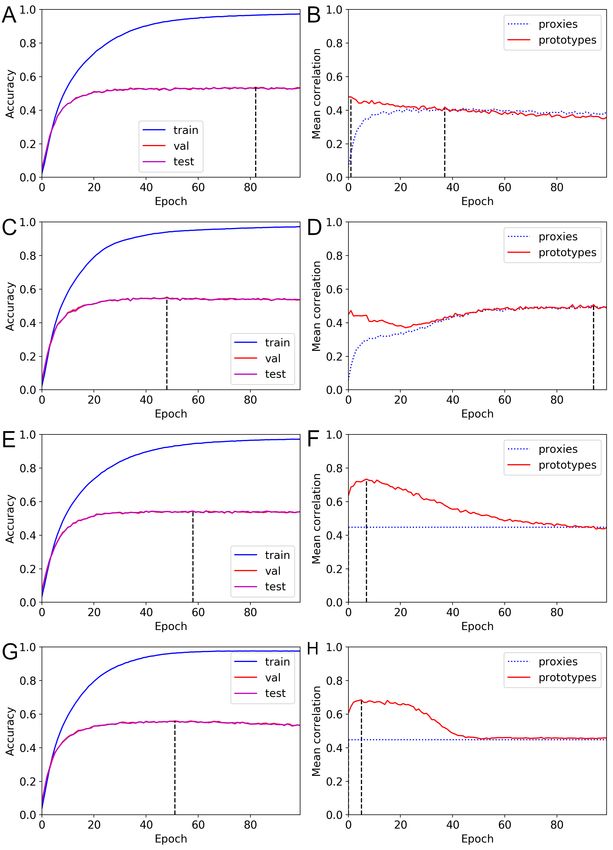
mini-batch B ⊆ D is defined as:
                                                          1       X
                                               LCE = −                       log(p(ci |xi )).                (3)
                                                         |B|
                                                               (xi ,ci )∈B

                   Metric learning
                   While softmax classifiers are commonly used in deep learning classification, metric
                   learning approaches can be beneficial, as they better control data points in embedding
                   space. Hence, metric learning can provide information on the similarity between
                   different data points. Metric learning approaches can be divided into two categories:
                   (direct) embedding-based methods and classification-based methods. Embedding-based
                   methods [19, 20] directly compare data points in embedding space to train an embedding
                   function (feature map) f (·). Because embedding-based methods compare data points
                   directly, they must be trained with pairs (using the contrastive loss) or triplets (using
                   the triplet loss) of data points. Thus, embedding-based methods have high training
                   complexity and require special mining algorithms [13] to prevent slow convergence
                   speeds [14]. On the other hand, classification-based methods [13, 15, 16, 21, 22] use class
                   representatives to represent classes. According to the classification loss (cross-entropy
                   loss), class representatives guide data points to converge to class-specific positions.
                   Classification-based methods converge faster than embedding-based methods due to
                   their reduced sampling complexity (training with single data points). In this paper, we
                   focus on classification-based metric learning methods.

                   NormFace
                   NormFace [13], which is also known as normalized softmax [23], modifies Eq. 2 in the
                   softmax classifier. NormFace was motivated by the normalization of features during
                   feature comparisons to improve face verification during the testing phase. To apply
                   normalization during both the testing and training phases, NormFace normalizes the
                   feature (embedding) vectors and weight vectors and uses a zero bias term. Previous
                   experiments on metric learning models [8] have shown that NormFace and its
                   variants [15, 16, 24] achieved competitive performance on metric learning tasks.
                                          v
                       We denote ṽ = kvk   for any nonzero vector v and the angle between vectors W̃y and
                   f˜(x) as θy . Then, as W̃y = 1 = f˜(x) , we obtain the following equation:

                                            W̃yT f˜(x) = W̃y      f˜(x) cos θy = cos θy .                    (4)

                   According to Eq. 4, the class probability p(c|x) estimated by NormFace can be
                   expressed as:

                                                 exp(sW̃cT f˜(x))     exp(s cos θc )
                                       p(c|x) = P                  = P                 ,                     (5)
                                                            T ˜
                                                   exp(sW̃y f (x))      exp(s cos θy )
                                                 y∈Y                            y∈Y

                   where s > 0 is a scaling factor. NormFace learns embeddings according to this
                   estimation and the cross-entropy loss in Eq. 3.
                       We next investigate the geometrical meaning of the NormFace classification results.
                   If a data point x is classified as belonging to class c by NormFace, according to Eq. 5,
                   we obtain exp(s cos θc ) ≥ exp(s cos θy ), i.e., cos θc ≥ cos θy . As the cosine function is a
                   monotonically decreasing function in the interval (0, π), we obtain θc ≤ θy . In terms of
                   angles, the normalized embedding vector f˜(x) is closer (or equally close) to W̃c than
                   W̃y . As we can classify data points using normalized weight vectors according to this

January 27, 2023                                                                                           4/49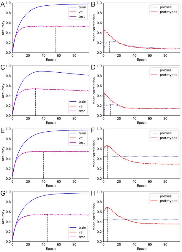
geometrical interpretation, we can consider W̃y as the class representative for a class
                   y ∈ Y. Fig. 2 visualizes the above explanation.

                   Fig 2. Visualization of NormFace classification results for two classes with
                   W̃1 =(0,1) and W̃2 =(1,0). As f˜(x) is closer to W̃1 than W̃2 , data point x is classified
                   as belonging to class 1.

                   Proxies and prototypes
                   Although NormFace [13] uses a learnable weight vector as a class representative for each
                   class, the average point for a class can also be used as a class representative. To prevent
                   confusion, we define two kinds of class representatives for each class: a proxy
                   representative and a prototype representative. We refer to the learnable weight vectors
                   as proxy representatives. In NormFace, the weight vectors W̃y are proxies. In this work,
                   the proxy representative are used to define the training loss and directly update the
                   network. Note that we can predefine the proxy representatives, and the proxies can be
                   fixed. On the other hand, we refer to the (normalized) average embedding for each class
                   as a prototype representative. We denote the average embedding for class y as vector
                   µy . In normalized space, this vector is defined as:

                                                             1 X ˜
                                                     µy =         f (x),
                                                            |Xy |
                                                                x∈Xy

                   where Xy ⊆ X is a set of data points in class y. Then, the prototype representatives are
                                     µ
                   defined as µ̃y = kµyy k . A metric learning method known as the prototypical network [9]
                   was devised for few-shot learning tasks. During the training process, this network uses
                   local prototypes based on special mini-batches known as episodes. In their work, the
                   authors used unnormalized average embedding as prototypes because they considered
                   Euclidean space. In this paper, we do not use prototypes for training, and (global)
                   prototypes using training data are used only for evaluation.
                       Note that the proxy and prototype representatives are not necessarily the same. For
                   instance, when we train the model with fixed proxies, the positions of the prototypes
                   change during training, while the positions of the proxies remain fixed. Moreover, the
                   confidence values are not necessarily maximized at the proxies [25]. In this case, the
                   data points may not converge to their proxies. This concept is explained further in the
                   next subsubsection.

                   SD softmax and DR formulation
                   In our previous work [25], we analyzed a softmax formulation for metric learning in
                   which negative squared distances were used as logit values. We called this formulation
                   the “softmax-based formulation” in our previous paper. In this work, we refer to this
                   formulation as “squared distance (SD) softmax” to prevent confusion with the standard
                   softmax formulation shown in Eq. 1.

January 27, 2023                                                                                        5/49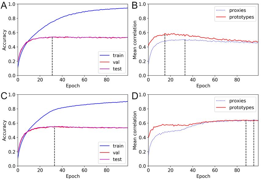
We denote the class representative for class y as Ry and the distance to class y as
                   dx,y := d(f (x), Ry ) according to the distance function d(·, ·). For the normalized
                   embeddings, we define dx,y := d(f˜(x), Ry ) by assuming that point Ry is normalized.
                   Then, the class probability p(c|x) estimated using the SD softmax formulation is:

                                                                exp(−d2x,c )
                                                      p(c|x) = P               .                                   (6)
                                                                  exp(−d2x,y )
                                                                 y∈Y

                   The SD softmax formulation uses the difference in the squared distance for training.
                     Consider the following equation:
                                             2           2              2
                               W̃y − f˜(x)       = W̃y       + f˜(x)         − 2W̃yT f˜(x) = 1 + 1 − 2 cos θy .

                   Then, we obtain:
                                                                      s                   2
                                                  s cos θy − s = −      W̃y − f˜(x)           .
                                                                      2
                   Thus, we obtain the equation:
                                                                                                            2
                             exp(s cos θc )       exp(s cos θc − s)      exp(− 2s W̃c − f˜(x) )
                            P                 = P                     = P                       2 ,                (7)
                               exp(s cos θy )       exp(s cos θy − s)             s        ˜
                           y∈Y                  y∈Y                        exp(− 2 W̃y − f (x) )
                                                                                   y∈Y

                   (This equation is taken from [13]). The above equation shows that the NormFace
                   formulation in Eq. 5 can be considered an SD softmax       formulation 6 that uses the
                   Euclidean distance on a hypersphere with radius 2s .
                                                                        p
                       In [25], we found that the SD softmax formulation had two main limitations. First,
                   the estimated probability and corresponding loss may be affected by scaling changes.
                   However, while this limitation must be considered when a Euclidean space is used, this
                   limitation can be addressed by using normalized embeddings, as in the NormFace
                   model [13]. The second limitation is that the estimated class probabilities are not
                   optimized at the class representatives. For instance, the maximum estimated class
                   probability p(c|x) is not found at the class representative of class c. The NormFace
                   model also encounters this issue. In the example shown in Fig. 2 with scaling factor
                   s = 2, point (− √12 , √12 ) is the point that maximizes the confidence value of class 1.
                       To address the above limitations, we proposed the distance ratio (DR)-based
                   formulation [25] for metric learning models. Mathematically, the DR formulation
                   estimates the class probability p(c|x) as:
                                                                  1
                                                                 ds             d−s
                                                                                 x,c
                                                   p(c|x) = P x,c1           = P −s .                              (8)
                                                                     dsx,y        dx,y
                                                               y∈Y              y∈Y

                   The DR formulation uses ratios of distances for training.
                       Moreover, the DR formulation [25] resolves the above two limitations of the SD
                   softmax formulation. In the example shown in Fig. 2, for any scaling factor s, point
                   (0, 1) = W̃1 is the point that maximizes the confidence value of class 1. Thus, our
                   experiments showed that the DR formulation has faster or comparable training speed in
                   Euclidean (unnormalized) embedding spaces.

January 27, 2023                                                                                                  6/49
Exponential moving average (EMA) approach
                   Zhe et al. [21] theoretically showed that, while training NormFace [13], the commonly
                   used gradient descent update method for the proxies based on the training loss cannot
                   guarantee that the updated proxies approach the corresponding prototypes. To address
                   this issue, they proposed using the normalized exponential moving average (EMA) to
                   update the proxies. Mathematically, when updating a proxy for a data point x in class
                   c, the proxy W̃c is updated as:

                                                            αf˜(x) + (1 − α)W̃c
                                                 W̃c :=                         ,                              (9)
                                                            αf˜(x) + (1 − α)W̃c

                   where 0 < α < 1 is a parameter that controls the speed and stability of the updates.
                   Their experimental results showed that the EMA approach achieved better performance
                   than the standard NormFace model on multiple datasets.

                   Adaptive scaling factor approach
                   Based on previous observations that the convergence and performance of NormFace
                   models [13] depend on the scale parameter s, Zhang et al. [22] proposed AdaCos, which
                   is a NormFace model trained by using the adaptive scale factor s in Eq. (5). Moreover,
                   they suggested to use parameter s, which significantly changes the probability p(c|x)
                   estimated by Eq. (5), where c is the class of data point x. In other words, they
                                                                            ∂p(c|x)(θc )
                   attempted to find a parameter s that maximizes              ∂θc         by approximating an s
                   value that satisfies the equation:

                                                          ∂ 2 p(c|x)(θc0 )
                                                                           = 0,                               (10)
                                                                ∂θc02

                   where θc0 := clip(θc , 0, π2 ) and clip(·, ·, ·) is a function that limits a value within a
                   specified range. They proposed two AdaCos models: static (fixed) and dynamic
                   versions. The static model determines a good scale parameter s before training the
                   NormFace model based on observations of the angles between the data points and
                   proxies. In the static model, the scale parameter s is not updated. The dynamic model
                   updates the scale parameter s during each iteration based on the current angles between
                   the data points and proxies.

                   CORR loss
                   In contrast to previous metric learning approaches that ignored hierarchical
                   relationships among classes, Barz and Denzler [5] used normalized embeddings to
                   achieve hierarchy-informed classification. First, they predefined the positions of the
                   proxies using a given hierarchical structure. These proxies are fixed, i.e., they are not
                   updated during training. Then, they used the predefined proxies to train the models
                   according to the CORR loss. For a data point x in class c, the CORR loss ensures that
                   the embedding vector f˜(x) is close to the corresponding proxy W̃c . The CORR loss of a
                   mini-batch B ⊆ D is defined as:
                                         1    X                          1  X
                              LCORR =                 1 − W̃cTi f˜(xi ) =            (1 − cos θci ),     (11)
                                        |B|                               |B|
                                            (xi ,ci )∈B                           (xi ,ci )∈B

                   where θci is the angle between W̃ci and f˜(xi ).

January 27, 2023                                                                                             7/49
Methods
                                   We investigated several methods and training options. The details of the settings are
                                   described in the following sections. The codes for our experiments will be available in
                                   https://github.com/hjk92g/Inspecting_Hierarchies_ML.

                                   Dataset We conducted experiments using three plankton datasets (small
                                   microplankton, large microplankton, and mesozooplankton) and two benchmark
                                   datasets (CIFAR100 [26] and NABirds [27]). Table 1 summarizes the number of classes
                                   and images in each dataset. The three plankton datasets were obtained from the
                                   Institute of Marine Research (IMR), where flow imaging microscopy is used during
                                   routine monitoring. The plankton samples were imaged using three FlowCams, ©2022
                                   Yokogawa Fluid Imaging Technologies, Inc., with different magnification settings. The
                                   three plankton datasets contain nonliving classes of artifacts and debris. Moreover,
                                   these datasets contain class names that are not in the WordNet database [11]. In
                                   addition, the three plankton datasets have severe class imbalances. For example, each
                                   class in the small microplankton (MicroS) dataset contains 1 to 456 images. Further
                                   details on the plankton datasets can be found in S2 Appendix. We randomly divided
                                   each plankton dataset into 70% training data, 10% validation data, and 20% test data.
                                   For the plankton datasets, we use images without any augmentation. As the input
                                   images have diverse image sizes, we resized the input images to 128 × 128. The
                                   CIFAR100 dataset contains 100 classes and 600 images per class. The CIFAR100
                                   contains 50000 training and 10000 test images, and we randomly divided the original
                                   training data into 45000 training and 5000 validation data. Furthermore, we applied
                                   random transformations (15 degree range rotations, 10% range translations, 10% range
                                   scaling, 10 degree range shearing, and horizontal flips) on the CIFAR100 training data.
                                   We did not resize images from their original size of 32 × 32. The NABirds dataset
                                   contains 23929 training and 24633 test images. Similar to the plankton datasets, we
                                   randomly divided this dataset into 70% training data, 10% validation data, and 20%
                                   test data. We resized the images to 128 × 128 pixels. We also applied the same
                                   augmentations applied to the CIFAR100 dataset on the NABirds dataset. The
                                   predefined hierarchical structures are available in S1 Appendix.

Table 1. Summary of the studied datasets.

                     Dataset        Target particle     Images per class     Images              Classes
                                  (plankton datasets)

            Small microplankton
                                      5 to 50 µm            1 to 456          6738                109
                 (MicroS)
            Large microplankton
                                    35 to 500 µm            2 to 613          8348                102
                 (MicroL)
              Mesozooplankton
                                   180 to 2000 µm           3 to 486          6738                 52
                 (MesoZ)
               CIFAR100 [26]              —                   600             60000               100

                   NABirds [27]           —                13 to 120          48562               555

                                   Models We consider four types of models: the softmax classifier, NormFace,
                                   ProxyDR (explained below), and a CORR loss-based model. We focus on metric
                                   learning models with normalized embeddings, as normalization is commonly used in
                                   metric learning models to improve performance [5, 13, 28]. ProxyDR is a model that uses

January 27, 2023                                                                                                      8/49
proxies for classification and DR formulations (8) to estimate class probabilities p(c|x).
Similar to the NormFace model, ProxyDR uses the Euclidean distance on a hypersphere.
The difference between the two models is that ProxyDR uses DR formulations, while
NormFace uses SD softmax formulations (as shown in Eq. 7). For the plankton
datasets, we used a pretrained Inception version 3 architecture [29] as the backbone.
For the CIFAR100 and NABirds datasets, we used a pretrained ResNet50 [30] as the
backbone. In addition to the backbones, we applied a learnable linear transformation to
obtain 128-dimensional embeddings f (x). For the plankton datasets, we incorporate the
T
size information. Specifically, when a data point x has size vsize = [width, height] , we
0 T
take the elementwise logarithm vsize = [log(width), log(height)] . By applying a linear
transformation, we obtain an embedding vector fsize (x) according to the size
T 0
information, i.e., fsize (x) = Wsize vsize + bsize , where Wsize is a learnable matrix with
2
shape 2 × 128 and bsize ∈ R is a learnable vector. Then, we add this vector to the
original embedding vector, namely, f (x) := f (x) + fsize (x).
Training settings We trained the models according to the backbone weights and
other weights (linear transformations, proxies). We used the Adam optimizer [31] with a
learning rate of 10−4 . Except in the case of a dynamic approach (explained below), we
use 10.0 as a scaling factor in both NormFace and ProxyDR. We set the training batch
size in all experiments to 32. For the plankton datasets, we trained the models for 50
epochs. For the CIFAR100 and NABirds datasets, we trained the models for 100 epochs.
During each epoch, we assessed the model accuracy. We chose the model with the
highest validation accuracy for testing. For each setting, we trained the models five
times with different seeds for the random split.
Training options The different training options are described as follows. The
dynamic approach affects the scale factors in Eqs. 5 and 8. The EMA and MDS
approaches both affect the proxy calculations.
• Standard: standard training with a fixed scale factor s = 10, with proxies updated
using the cross-entropy loss (3).
• EMA (exponential moving average): training using the normalized exponential
moving average [21], as shown in Eq. 9, to update the proxies. When multiple
data points have the same class c in a mini-batch, we apply a modified expression.
Specifically, instead of applying the EMA using a single data point, as in Eq. 9,
we use the normalized average embedding (local prototype) of the mini-batch.
Mathematically, when updating a proxy for m data points xB;1 , · · · , xB;m with
class c in mini-batch B, the normalized average embedding is defined as:
m
f˜(xB;i )
P
i=1
µ̃B;c = m
.
f˜(xB;i )
P
i=1
Then, proxy W̃c is updated as:
αµ̃B;c + (1 − α)W̃c
W̃c := , (12)
αµ̃B;c + (1 − α)W̃c
where α is the same parameter as in Eq. 9. We set the parameter α to 0.001.
January 27, 2023 9/49• Dynamic: training with a dynamic scale factor, similar to AdaCos [22]. In
contrast to the original paper, which chooses a scale factor using an approximate
expression, we use the Adam [31] optimizer to determine a scale factor that
satisfies Eq. 10. More details are included in S1 Appendix.
• MDS (multidimensional scaling): training according to predefined hierarchical
information. We use the hierarchical information to set (fixed) proxies. First, as
in the distance calculation method in the problem setting subsection, we use a
predefined hierarchy to generate a distance matrix. We denote the (hierarchical)
distance between the ith and jth classes
√
as dH (i, j). For each hierarchical distance
2dH
dH , we apply a transformation dT = β+dH for a scalar β > 0 to address the
√
limited Euclidean distance (≤ 2) on unit spherical spaces. We set β = 1.0 √
in all
2d
of our experiments. (Note that if d is a metric, the transformed distance β+d is
also a metric.) Then, according to the transformed distance matrix DT , we use
multidimensional scaling (MDS) to set the proxies. Mathematically, we minimize
a value known as the normalized stress, which can be expressed as:
kDW̃ − DT kF
Stress(DW̃ ) := , (13)
kDT kF
where DW̃ is a pairwise Euclidean distance matrix according to proxies W̃y and
k·kF is the Frobenius norm. We use the Adam optimizer with a learning rate of
10−3 for 1000 iterations to obtain the proxies. While we used stochastic gradient
descent for the MDS option, different methods, such as those applied by Barz and
Denzler [5], can also be used for MDS. During training, we fix the obtained
proxies and update only the embedding function f (·).
Performance measures In our experiments, we consider three types of performance
measures: standard classification measures, hierarchical inference performance measures,
and hierarchy-informed performance measures. The hierarchical inference performance
measures are used to estimate how well the learned class representatives match the
predefined hierarchies. The hierarchy-informed performance measures are used to
estimate how well a model performs on classification or similarity measures according to
the predefined hierarchies.
We used the top-k accuracy as a standard classification measure, the mean
correlation as the hierarchical inference performance measure, and the average
hierarchical distance (AHD), hierarchical precision at k (HP@k), hierarchical similarity
at k (HS@k), and average hierarchical similarity at k (AHS@k) as hierarchy-informed
performance measures. The utilized measures are defined as follows.
• Top-k accuracy: The classification accuracy was calculated, with correct
classification defined as whether the labeled class is in the top-k predictions (most
likely classes), i. e., the k classes with the highest confidence values. We report
results for k = 1, 5.
• Mean correlations: We introduce this measure to evaluate how well the learned
class representatives match the predefined hierarchical structure. We obtain the
class representatives (either proxies or prototypes) from the learned model using
training data points. Then, we obtain the pairwise distance matrix DL based on
the class representatives. We compare matrix DL with the distance matrix DH
based on the predefined hierarchical structure. Specifically, for each class (row),
we calculate Spearman’s rank correlation coefficient according to the two matrices.
January 27, 2023 10/49Then, we determine the mean correlation using Fisher transformations. More
precisely, we apply a Fisher transformation arctanh(·) on each correlation
coefficient, take the average of the transformed values, and apply tanh(·) on the
average value.
For the plankton datasets, the predefined hierarchical structures of the living
classes are based on biological taxonomies. However, these datasets also contain
some nonliving classes, such as “large bubbles” and “dark debris”. Considering
that the predefined hierarchical structures of the living classes are scientifically
defined, for the plankton datasets, we report mean correlations among whole
classes or only among living classes.
• AHD: The average hierarchical distance of the top-k predictions [4] was calculated
as the average hierarchical distance dH between the labeled classes and each of
the top-k most likely classes. In contrast to Bertinetto et al. [4], who considered
only misclassified cases, we consider all cases. Hence, in our calculations, the final
denominators differ. When k = 1, the AHD measure is the same as the average
hierarchical cost (AHC) measure defined by Garnot and Landrieu [6]. We report
results for k = 1, 5.
• HP@k: The hierarchical precision at k [32] was taken as a performance measure.
Specifically, let us denote a (hierarchical) neighborhood set of a class c with the
distance threshold as N (c, ), i.e., n ∈ N (c, ) ⇐⇒ dH (c, n) ≤ . We define
hCorrectSet(c, k) as the neighborhood set N (c, ) with the smallest such that
|hCorrectSet(c, k)| ≥ k. Then, the hierarchical precision at k is calculated as the
fraction of the top-k predictions in hCorrectSet(c, k). We report the results for
k = 5.
• HS@k: The hierarchical similarity at k is a measure that was introduced by Barz
and Denzler [5] with the name “hierarchical precision at k”, although this metric
does not evaluate precision and instead assesses similarity. Here, we use a different
measure with the same name that was defined by Frome et al. [32]. Hence, we
renamed the measure “hierarchical similarity at k”. When c is a label of a query
data point x, let R = ((x1 , c1 ) , · · · , (xm , cm )) be the ordered list of image-label
pairs based on the distance (sorted by ascending distance) to point x in the
2
normalized embedding space. Considering cos(θ) = 1 − ku1 −u 2
2k
, where u1 and u2
are unit vectors and θ is the angle between u1 and u2 , we defined the similarity
between the ith and jth classes sH (i, j) as:
dT (i, j)2
sH (i, j) = 1 − , (14)
2
where i and j are the indices for classes (1 ≤ i, j ≤ |Y|).
The hierarchical similarity at k is then defined as:
k
P
sH (I(c), I(ci ))
i=1
HS@k := k
, (15)
P
maxπ sH (I(c), I(cπi ))
i=1
where I(·) is an index function that outputs the corresponding index (between 1
and |Y|) for a class and π is an index permutation that ranges from 1 to m. We
report results for k = 50, 250.
• AHS@K: The average hierarchical similarity at K was introduced by Barz and
Denzler [5] as the “average hierarchical precision at K”. Due to similar reasons as
January 27, 2023 11/49for HS@k, we renamed the measure. The average hierarchical similarity at K is
defined as the area under the curve of HS@k from k = 1 to k = K. We report
results for K = 250.
Results
Main results
The performance measure evaluation results are shown in bar plots with 95% confidence
intervals. Dashed lines separate models trained with or without predefined hierarchical
knowledge. We show only the results on the CIFAR100 and NABirds datasets in the
main text. All results are included in S3 Appendix. To reduce spurious findings, we
focus on consistent trends across the five datasets.
Figs. 3 and 4 and the figures in S3 Appendix show the top-k accuracy for various
training settings. The NormFace and ProxyDR models achieved comparable top-k
accuracy for both k values on most datasets. The softmax loss model obtained low
top-k accuracy. While the result was not significant, using the dynamic option achieved
higher top-1 accuracy than standard training. When the EMA option was added to the
standard and dynamic options, the top-5 accuracy decreased, except for standard
NormFace on the NABirds dataset. While the CORR loss achieved top-1 accuracy that
was comparable to that achieved by other training options with predefined hierarchical
information, this model obtained low top-5 accuracy on all datasets. The top-5 accuracy
with the CORR loss was even lower than that with the softmax loss, except on the
NABirds dataset. Although the results were better than those of the CORR loss model,
the use of predefined hierarchical information during training for NormFace and
ProxyDR also reduced the top-5 accuracy. These results show the opposite trend to the
changes in the top-1 accuracy, which showed comparable or enhanced performance.
Moreover, the dynamic MDS approach obtained lower top-5 accuracy than the MDS
approach without the dynamic option.
Fig 3. Top-k accuracy results (A: k = 1, B: k = 5) on the CIFAR100 dataset.
January 27, 2023 12/49Fig 4. Top-k accuracy results (A: k = 1, B: k = 5) on the NABirds dataset.
Figs. 5 and 6 and the figures in S3 Appendix show the mean correlation values for
various training options. When we consider training options that do not use predefined
hierarchical information, ProxyDR obtains higher mean correlations than NormFace,
except for the EMA approaches. The ProxyDR model with the dynamic option
obtained higher mean correlations than the standard ProxyDR model. As expected, the
use of predefined hierarchical information greatly increased the mean correlations based
on prototypes in both the NormFace and ProxyDR models, except the ProxyDR model
on the NABirds dataset. When we consider training options that utilize predefined
hierarchical information, the CORR loss model achieved the highest mean correlations
based on prototypes in most cases. The ProxyDR model typically achieved the
second-best mean correlations.
Fig 5. Correlation measures on the CIFAR100 dataset. (A) Values using
proxies. (B) Values using prototypes. The mean correlation value based on proxies with
the MDS option was 0.8580.
January 27, 2023 13/49Fig 6. Correlation measures on the NABirds dataset. (A) Values using proxies.
(B) Values using prototypes. The mean correlation value based on proxies with the
MDS option was 0.4476 (this value is small because the dataset contains 555 classes and
the embedding dimension is 128.).
Figs. 7 and 8 and the figures in S3 Appendix show the hierarchical performance
measures obtained with various training options. The softmax loss option achieved the
worst hierarchical performance, except for AHS@50 on the NABirds dataset. Although
these measures are used to assess the hierarchy-informed performance, some of the
measures are not substantially affected by the use of predefined hierarchical information
during training. For instance, the use of predefined hierarchical information in the
CIFAR100 dataset (Fig. 7) did not show noticeable improvements in terms of the AHD
(k=1), HS@50, and AHS@250 measures. Moreover, while the use of predefined
hierarchical information significantly improved the HS@250 results on most datasets,
only marginal improvements were observed for the CIFAR100 dataset. On the other
hand, the use of predefined hierarchical information significantly improved the AHD
(k=5) and HP@5 results on all datasets. The CORR loss achieved the best results on
these two measures, except on the NABirds dataset. Adding the dynamic option to the
standard and MDS options improved performance on these two measures, except for the
ProxyDR model on the CIFAR100 dataset. When we consider training options that do
not use predefined hierarchical information, the ProxyDR model shows better
performance than NormFace in terms of these two measures, except for the EMA and
dynamic options on the CIFAR100 dataset. Under the same settings, ProxyDR
performed better than NormFace in terms of the HS@250 measure, except for the EMA
option on the CIFAR100 dataset. Moreover, under the same settings, the ProxyDR
model with the dynamic option achieved the highest HS@250 and AHS@250 values
among the compared models.
January 27, 2023 14/49Fig 7. Hierarchical performance measures on the CIFAR100 dataset. The
symbol ↓ denotes that lower values indicate better performance. The symbol ↑ denotes
that higher values indicate better performance. (A) AHD (k=1): ↓. (B) AHD (k=5): ↓.
(C) HP@5: ↑. (D) HS@50: ↑. (E) HS@250: ↑. (F) AHS@250: ↑.
January 27, 2023 15/49Fig 8. Hierarchical performance measures on the NABirds dataset. The
symbol ↓ denotes that lower values indicate better performance. The symbol ↑ denotes
that higher values indicate better performance. (A) AHD (k=1): ↓. (B) AHD (k=5): ↓.
(C) HP@5: ↑. (D) HS@50: ↑. (E) HS@250: ↑. (F) AHS@250: ↑.
Additional mean correlation results
To investigate the changes in the class representatives, we evaluated the mean
correlations at the end of each training epoch. We report only the results on the
CIFAR100 and NABirds datasets. Moreover, we report results for ProxyDR models
with the standard and dynamic options. More results are included in S3 Appendix.
Furthermore, we report mean correlations based on random networks, i.e., networks with
random weights, pretrained networks, and unnormalized and normalized input spaces.
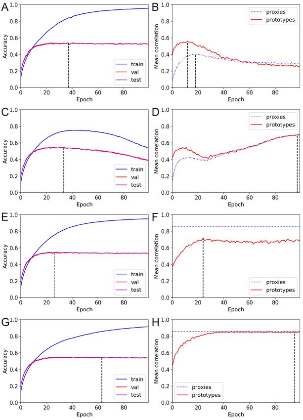
Figs. 9 and 10 visualize the changes in the mean correlation values during ProxyDR
model training (averaged values from five different seeds). Surprisingly, we found that
the prototypes of the approximately untrained networks (pretrained on ImageNet [3]
and trained on the target dataset, e.g., CIFAR100 or NABirds, for only one epoch)
already have relatively high correlations (approximately 0.4), with predefined
hierarchical structures. While the accuracy curves show no noticeable differences, using
the dynamic option modified the transition in the mean correlations. In particular,
January 27, 2023 16/49prototype-based mean correlations increased after 20 to 40 training epochs, and the
maximum values were obtained near the end of training (approximately 100 epochs).
The proxy-based mean correlations started at low values, and the difference with the
prototype-based mean correlations was reduced. Moreover, the training epoch during
which the validation accuracy is maximized often differs from the training epoch during
which the correlation measures are maximized.
Fig 9. Changes in accuracy and mean correlations for the CIFAR100
dataset (ProxyDR). (A) Accuracy curve with standard training. (B) Mean
correlation curve with standard training. (C) Accuracy curve with the dynamic option.
(D) Mean correlation curve with the dynamic option.
January 27, 2023 17/49Fig 10. Changes in accuracy and mean correlations for the NABirds
dataset (ProxyDR). (A) Accuracy curve with standard training. (B) Mean
correlation curve with standard training. (C) Accuracy curve with the dynamic option.
(D) Mean correlation curve with the dynamic option.
Table 2 shows prototype-based mean correlation values and their 95 percent
confidence intervals based on five different seeds. The mean correlations with the
random networks show that the prototypes and ground-truth hierarchy are correlated.
While these values are smaller than the other cases shown in the table, the results show
that random networks have some degree of semantic understanding.
Table 2. Mean correlations based on prototypes.
Space Random weights Pretrained Input space Normalized input space
CIFAR100 0.2841 ± 0.0303 0.3816 ± 0.0116 0.3414 ± 0.0353 0.2609 ± 0.0416
NABirds 0.1088 ± 0.0839 0.2648 ± 0.0349 0.1740 ± 0.0056 0.2369 ± 0.0039
“Random weights” and “pretrained” mean embedding space based on the ResNet50 [30] backbone.
Discussion
In this work, we investigate classification and hierarchical performance under different
models and training options. Our experiments reveal several important findings. Under
the training options that do not consider predefined hierarchical information, the
ProxyDR model achieved better hierarchical inference performance than NormFace in
most cases. Furthermore, under the same training options, ProxyDR achieved better
hierarchy-informed performance in terms of the AHD (k=5) and HP@5 measures.
Moreover, we observed that the use of a dynamic scaling factor improved the
hierarchical inference performance. The changes in the mean correlation values (Figs. 9
January 27, 2023 18/49and 10) verified the effect of the dynamic training option. These results reveal the
importance of dynamic training approach. We also found that some hierarchy-informed
performance measures are not significantly improved by the use of known hierarchical
structures. This finding indicates that multiple hierarchy-informed performance
measures should be considered to compare the hierarchy-informed performance of
different models. We also observed a trade-off between the hierarchy-informed
performance and top-5 accuracy. While the CORR loss model typically achieved the
best hierarchical performance, this model obtained the lowest top-5 accuracy among the
experimental models. Similarly, the use of predefined hierarchical information in
NormFace and ProxyDR significantly improved the AHD (k=5) and HP@5 performance
but reduced the top-5 accuracy. In contrast to previous works that observed a trade-off
between hierarchy-informed performance and top-1 accuracy [4], we did not observe this
trade-off with top-1 accuracy.
Surprisingly, we found that prototypes based on CNNs with random weights showed
correspondence with predefined hierarchies that was higher than random chance.
Because CNNs combine convolutional and pooling layers, most CNN architectures have
translation invariance properties. Because of such priors, random networks may know
weak perceptual similarity [33]. Another possible reason for this result is that
prototypes of input spaces show higher correspondence with predefined hierarchies than
random chance. The Johnson-Lindenstrauss lemma [34] shows that linear projections
using random matrices approximately preserve distances. If this property holds for
nonlinear projections based on random neural networks, network-based prototypes may
also correspond to predefined hierarchies. This phenomenon suggests that when we use
metric learning models with proxies, the proxies can be assigned based on prototypes
instead of starting at random positions. This may improve training during the initial
epochs, as we start from proxies that are more semantically reasonable than random
positions.
Although we observed that the DR formulation improves the hierarchical inference
performance and hierarchy-informed performance when training models without
predefined hierarchies, we did not study the reasons underlying these phenomena. We
suggest one possible hypothesis. While NormFace prevents sudden changes in the
scaling factor by using normalized embeddings, its loss function is based on the squared
difference of the distance (as it uses the SD softmax formulation). As this loss can
increase the squared difference of the distance among different proxies, the absolute
distance between any pairs of proxies may be increased. This tendency can result in
larger distances, even among semantically similar classes, and proxy positions that are
less organized in terms of visual similarity. On the other hand, the DR
formulation-based loss is based on distance ratios. Thus, there is no tendency to
increase absolute distances among proxies, and proxies can be structured according to
visual similarity. However, further investigations are needed to verify this hypothesis
and reveal the underlying cause.
Conclusion
The hierarchy-informed performance must be improved to more broadly adopt
classification models. We explored this concept with classification-based metric learning
models in situations in which hierarchical information is and is not available during
training. Our results show that when the class hierarchical relations are unknown, the
ProxyDR model achieves the best hierarchical inference and hierarchy-informed
performance. In contrast, with hierarchy-informed training, the CORR loss model
achieves the best hierarchy-informed performance but the lowest top-5 accuracy on most
datasets. Since some hierarchy-informed measures may not be improved by the use of
January 27, 2023 19/49hierarchical information during training, multiple hierarchy-informed performance
measures should be used to obtain appropriate comparisons. Additionally, our
experiments reveal that during classification-based metric learning, initializing proxies
based on prototypes may be beneficial.
Acknowledgments
Hyeongji Kim, Terje Berge, and Ketil Malde acknowledge the Ministry of Trade,
Industry and Fisheries for financial support. The authors thank Gayantonia Franze,
Hege Lyngvær Mathisen, Magnus Reeve, and Mona Ring Kleiven, from the Plankton
Research Group at Institute of Marine Research (IMR), for their contributions to the
plankton datasets.
References
1. He K, Zhang X, Ren S, Sun J. Delving deep into rectifiers: Surpassing
human-level performance on imagenet classification. In: Proceedings of the IEEE
international conference on computer vision; 2015. p. 1026–1034.
2. Russakovsky O, Deng J, Su H, Krause J, Satheesh S, Ma S, et al. Imagenet large
scale visual recognition challenge. International journal of computer vision.
2015;115(3):211–252.
3. Deng J, Dong W, Socher R, Li LJ, Li K, Fei-Fei L. Imagenet: A large-scale
hierarchical image database. In: 2009 IEEE conference on computer vision and
pattern recognition. Ieee; 2009. p. 248–255.
4. Bertinetto L, Mueller R, Tertikas K, Samangooei S, Lord NA. Making better
mistakes: Leveraging class hierarchies with deep networks. In: Proceedings of the
IEEE/CVF Conference on Computer Vision and Pattern Recognition; 2020. p.
12506–12515.
5. Barz B, Denzler J. Hierarchy-based image embeddings for semantic image
retrieval. In: 2019 IEEE Winter Conference on Applications of Computer Vision
(WACV). IEEE; 2019. p. 638–647.
6. Garnot VSF, Landrieu L. Leveraging Class Hierarchies with Metric-Guided
Prototype Learning. In: British Machine Vision Conference (BMVC); 2021.
7. Jayathilaka M, Mu T, Sattler U. Ontology-based n-ball concept embeddings
informing few-shot image classification. arXiv preprint arXiv:210909063. 2021;.
8. Musgrave K, Belongie S, Lim SN. A metric learning reality check. In: European
Conference on Computer Vision. Springer; 2020. p. 681–699.
9. Snell J, Swersky K, Zemel R. Prototypical Networks for Few-shot Learning.
Advances in Neural Information Processing Systems. 2017;30:4077–4087.
10. Chen WY, Liu YC, Kira Z, Wang YCF, Huang JB. A closer look at few-shot
classification. arXiv preprint arXiv:190404232. 2019;.
11. Miller GA. WordNet: An electronic lexical database. MIT press; 1998.
12. Godbole S. Exploiting confusion matrices for automatic generation of topic
hierarchies and scaling up multi-way classifiers. Annual Progress Report, Indian
Institute of Technology–Bombay, India. 2002;.
January 27, 2023 20/4913. Wang F, Xiang X, Cheng J, Yuille AL. Normface: L2 hypersphere embedding for
face verification. In: Proceedings of the 25th ACM international conference on
Multimedia; 2017. p. 1041–1049.
14. Kim S, Kim D, Cho M, Kwak S. Proxy anchor loss for deep metric learning. In:
Proceedings of the IEEE/CVF Conference on Computer Vision and Pattern
Recognition; 2020. p. 3238–3247.
15. Wang H, Wang Y, Zhou Z, Ji X, Gong D, Zhou J, et al. Cosface: Large margin
cosine loss for deep face recognition. In: Proceedings of the IEEE conference on
computer vision and pattern recognition; 2018. p. 5265–5274.
16. Deng J, Guo J, Xue N, Zafeiriou S. Arcface: Additive angular margin loss for
deep face recognition. In: Proceedings of the IEEE/CVF Conference on
Computer Vision and Pattern Recognition; 2019. p. 4690–4699.
17. Wan A, Dunlap L, Ho D, Yin J, Lee S, Petryk S, et al. {NBDT}: Neural-Backed
Decision Tree. In: International Conference on Learning Representations;
2021.Available from: https://openreview.net/forum?id=mCLVeEpplNE.
18. Silla CN, Freitas AA. A survey of hierarchical classification across different
application domains. Data Mining and Knowledge Discovery. 2011;22(1):31–72.
19. Weinberger KQ, Blitzer J, Saul L. Distance metric learning for large margin
nearest neighbor classification. Advances in neural information processing
systems. 2005;18.
20. Hadsell R, Chopra S, LeCun Y. Dimensionality reduction by learning an
invariant mapping. In: 2006 IEEE Computer Society Conference on Computer
Vision and Pattern Recognition (CVPR’06). vol. 2. IEEE; 2006. p. 1735–1742.
21. Zhe X, Ou-Yang L, Yan H. Improve L2-normalized Softmax with Exponential
Moving Average. In: 2019 International Joint Conference on Neural Networks
(IJCNN). IEEE; 2019. p. 1–7.
22. Zhang X, Zhao R, Qiao Y, Wang X, Li H. Adacos: Adaptively scaling cosine
logits for effectively learning deep face representations. In: Proceedings of the
IEEE/CVF Conference on Computer Vision and Pattern Recognition; 2019. p.
10823–10832.
23. Zhai A, Wu HY. Classification is a strong baseline for deep metric learning.
British Machine Vision Conference (BMVC). 2019;.
24. Liu W, Wen Y, Yu Z, Li M, Raj B, Song L. Sphereface: Deep hypersphere
embedding for face recognition. In: Proceedings of the IEEE conference on
computer vision and pattern recognition; 2017. p. 212–220.
25. Kim H, Parviainen P, Malde K. Distance-Ratio-Based Formulation for Metric
Learning. arXiv preprint arXiv:220108676. 2022;.
26. Krizhevsky A. Learning multiple layers of features from tiny images; 2009.
27. Van Horn G, Branson S, Farrell R, Haber S, Barry J, Ipeirotis P, et al. Building
a bird recognition app and large scale dataset with citizen scientists: The fine
print in fine-grained dataset collection. In: Proceedings of the IEEE Conference
on Computer Vision and Pattern Recognition; 2015. p. 595–604.
January 27, 2023 21/4928. Movshovitz-Attias Y, Toshev A, Leung TK, Ioffe S, Singh S. No fuss distance
metric learning using proxies. In: Proceedings of the IEEE International
Conference on Computer Vision; 2017. p. 360–368.
29. Szegedy C, Vanhoucke V, Ioffe S, Shlens J, Wojna Z. Rethinking the inception
architecture for computer vision. In: Proceedings of the IEEE conference on
computer vision and pattern recognition; 2016. p. 2818–2826.
30. He K, Zhang X, Ren S, Sun J. Deep residual learning for image recognition. In:
Proceedings of the IEEE conference on computer vision and pattern recognition;
2016. p. 770–778.
31. Kingma DP, Ba J. Adam: A method for stochastic optimization. arXiv preprint
arXiv:14126980. 2014;.
32. Frome A, Corrado GS, Shlens J, Bengio S, Dean J, Ranzato M, et al. Devise: A
deep visual-semantic embedding model. Advances in neural information
processing systems. 2013;26.
33. Zhang R, Isola P, Efros AA, Shechtman E, Wang O. The unreasonable
effectiveness of deep features as a perceptual metric. In: Proceedings of the IEEE
conference on computer vision and pattern recognition; 2018. p. 586–595.
34. Johnson W, Lindenstrauss J. Extensions of Lipschitz mappings into a Hilbert
space. Contemporary Mathematics. 1984;26:189–206.
January 27, 2023 22/49Supporting information
S1 Appendix
Detailed explanation of the dynamic (adaptive) scaling factors
in the NormFace and ProxyDR models.
Zhang et al. [22] rewrote Eq. 5 as follows:
exp(s cos θc )
p(c|x) = ,
exp(s cos θc ) + Bx
P
where c is the corresponding class of point x and Bx = exp(s cos θy ). They
y6=c,y∈Y
to π2 during the training
found that θy was closeP P process for y 6= c, i.e., for different
classes. Thus, Bx ≈ exp(s cos π2 ) = exp(0) = |Y| − 1.
y6=c,y∈Y y6=c,y∈Y
∂ 2 p(c|x)(θc )
In Eq. 10, ∂θc2 can be written as:
∂ 2 p(c|x)(θc ) −sBx exp(s cos θc )ψN ormF ace (s, θc )
= 3 ,
∂θc2 (exp(s cos θc ) + Bx )
where ψN ormF ace (s, θc ) = cos θc (exp(s cos θc ) + Bx ) + s sin2 θc (exp(s cos θc ) − Bx ).
Moreover, they used s = log Bx
cos θc to approximate the solution for Eq. 10. For the static
version, they used |Y| − 1 to estimate Bx and π4 to estimate θc . For the dynamic
version, they used Bx;avg to estimate Bx and θc;med to estimate θc , where Bx;avg is the
average of Bx in a mini-batch and θc;med is the median of the θc values in a mini-batch.
They clipped the θc;med value to be in the range 0, π4 .
Instead of using s = log Bx
cos θc , in our implementation, we use the Adam optimizer [31]
2
to update a scale factor s that minimizes ψN ormF ace (s, θc ), i.e., ψN ormF ace (s, θc ) ≈ 0.
For ψN ormF ace (s, θc ), we use |Y| − 1 to estimate Bx and π4 to estimate θc to initialize
the value of s. During model training, we use Bx;avg to estimate Bx and θc;med to
estimate θc .
We can also apply the dynamic scaling factor to the ProxyDR model. First, we
define dx,y := f˜(x) − W̃y . We rewrite Eq. 8 as:
d−s
x,c
p(c|x) = ,
d−s
x,c + Bx
d−s π
P
where Bx = x,y . Assuming θy ≈ 2 for y 6= c, we obtain
y6=c,y∈Y
π −s
−s
= (|Y| − 1) π2
P
Bx ≈ 2 .
y6=c,y∈Y
2
The expression ∂ p(c|x)(θ
∂θc2
c)
can be written as:
(s−2)
∂ 2 p(c|x)(θc ) Bx sθc ψP roxyDR (s, θc )
2
= 3
∂θc (Bx θcs + 1)
where ψP roxyDR (s, θc ) = Bx (s + 1)θcs − s + 1. We then use the Adam optimizer to
update a scale factor s that minimizes ψP2 roxyDR (s, θc ).
January 27, 2023 23/49S2 Appendix
Dataset details.
All plankton images were obtained using FlowCam (Yokogawa Fluid Imaging
Technologies). FlowCam is a flow imaging microscope that captures particles flowing
through glass flowcells with well-defined volumes. The three plankton datasets were
obtained according to different types of samples (live and Lugol fixed whole seawater or
180 µm WP2 plankton net samples) using three different FlowCams (FlowCam 8400,
FlowCam VS, and FlowCam Macro) with various magnifications. Thus, the datasets
include particles ranging from 5 to 2000 µm in size, thus representing nano-, micro-, and
mesozooplankton. The plankton samples were obtained from three coastal monitoring
stations (Institute of Marine Research) along the Norwegian coast, including Holmfjord
in the north, Austevoll in the west and Torungen in the south. In addition, for the nano-
and microplankton, seawater samples were obtained from a tidal zone at a depth of 1
meter at the research station at Flødevigen in southern Norway, which is approximately
2 nautical miles from the southern monitoring station at Torungen. The sampling period
for the three datasets covered all seasons over a period of approximately 2.5 years.
Small microplankton (MicroS) This dataset contains images of fixed and live
seawater samples acquired at a depth of 5 m at the three monitoring stations and a
depth of 1 m in the tidal zone (see above). The seawater samples were carefully filtered
through a 80 µm mesh to ensure that 100 µm flowcell was not clogged and imaged using
a 10× objective. This FlowCam configuration results in a total magnification of 100×
and images particles ranging from 5 to 50 µm. Before resizing, one pixel in an image
represented 0.7330 µm.
Large microplankton (MicroL) This dataset contains images of fixed and live
seawater samples acquired at a depth of 5 m at the three monitoring stations and a
depth of 1 m in the tidal zone (see above). The seawater samples were not filtered and
were imaged using a 2× objective, targeting 35 to 500 µm particles. Before resizing, one
pixel in an image represented 2.9730 µm. Due to instrument repair and adjustments to
improve image quality, the camera settings were modified during the 3 years of imaging
to acquire this dataset. Therefore, the image appearance and quality are slightly
variable.
Mesozooplankton (MesoZ) This dataset contains images of mesozooplankton
samples acquired at the three coastal monitoring stations (see above) and a transect in
the Norwegian Sea (Svinøysnittet). The samples were obtained using an IMR (Institute
of Marine Research) standard plankton net (WP2) or a multinet mammoth (both
180 µm mesh) and fixed with 4% formaldehyde. The images were acquired by two
FlowCam instruments (one in Bergen and one in Flødevigen), and the image
appearance differs slightly between the two instruments. The FlowCam macro was
equipped with a 0.5× objective, resulting in a total magnification of 12.5 and imaging
organisms ranging from 180 to 2000 µm. Before resizing, one pixel in an image
represented 9.05 µm. All images in the mesozooplankton dataset are in grayscale.
NABirds Data provided by the Cornell Lab of Ornithology, with thanks to
photographers and contributors of crowdsourced data at AllAboutBirds.org/Labs.
This material is based upon work supported by the National Science Foundation under
Grant No. 1010818.
January 27, 2023 24/49You can also read