Insight Into Supersonic Combustion Using High-order Simulations - Research ...
←
→
Page content transcription
If your browser does not render page correctly, please read the page content below
Insight Into Supersonic Combustion Using High- order Simulations Ioannis Kokkinakis University of Nicosia Dimitris Drikakis ( drikakis.d@unic.ac.cy ) University of Nicosia Yun-qin He Beihang University Guo-zhu Liang Beihang University Research Article Keywords: supersonic combustion, high-order simulations, Propulsion, scramjet technologies Posted Date: January 7th, 2022 DOI: https://doi.org/10.21203/rs.3.rs-1214905/v1 License: This work is licensed under a Creative Commons Attribution 4.0 International License. Read Full License
Insight into supersonic combustion using
high-order simulations
Ioannis W. Kokkinakis1 , Dimitris Drikakis1,* , Yun-qin He2 , and Guo-zhu Liang2
1 University of Nicosia, Nicosia CY-2417, Cyprus
2 Beihang University, Beijing 100191, China
* drikakis.d@unic.ac.cy
ABSTRACT
High-order simulations of supersonic combustion are presented to advance understanding of the complex chemically-reacting
flow processes and identify unknown mechanisms of the high-speed combustion process. We have employed 11th-order
accurate implicit large-eddy simulations in conjunction with thermochemistry models comprising 20 chemical reactions. We
compare the computations with available experiments and discuss the accuracy and uncertainties in both. Jets emanating from
above and below the hydrogen plumes influence the combustion process and accuracy of the predictions. The simulations
reveal that high temperatures are sustained for a long-distance downstream of the combustion onset. A barycentric map
for the Reynolds stresses is employed to analyse the turbulent anisotropy. We correlate the axisymmetric contraction and
expansion of turbulence with the interaction of reflected-shock waves with the supersonic combustion hydroxyl production
regions. The physics insights presented in this study could potentially lead to more efficient supersonic combustion and
scramjet technologies.
Introduction
Propulsion is one of the critical components for achieving sustainable future hypersonic flights. Turbojets have been successfully
used in aircraft flying in the transonic and supersonic region up to Mach 3. However, conventional aero-propulsion engines (e.g.,
turbofan & turbojet) cannot withstand temperatures occurring at higher speeds. Alternatively, ramjets can be used for Mach
numbers in the range of 3 to 5. Although the vehicle’s speed is supersonic, the engine design forces the flow to become subsonic
through a series of shockwaves and compression waves. This results in high pressures and temperatures, thus eliminating the
need for a compressor altogether prior to the combustion of the fuel. When increasing the flight speed yet further, eventually
the ramjet too becomes inefficient because the losses in the engine dramatically increase – the inlet temperature gets closer to
the exhaust temperature so less energy can be extracted in the form of thrust. The simplest alternative, therefore, is for the
incoming air to not be compressed (and hence heated) as much. Consequently, however, the air flowing through the combustion
chamber will still be travelling very fast relative to the engine. In fact, the flow in the combustion chamber will be supersonic
–hence the name supersonic-combustion ramjet, or scramjet–, resulting in a low temperature air that rapidly mixes with the fuel.
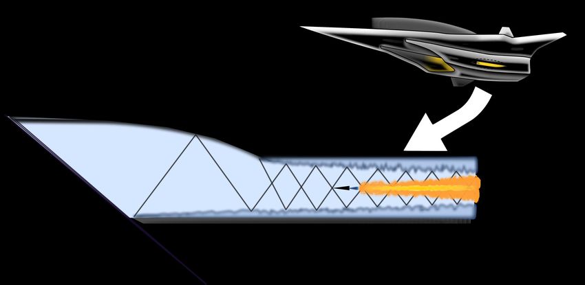
The whole reaction process is completed inside the engine, e.g., Fig 1. As per above, scramjet engines typically allow for Mach
speeds in the range of 6 to 15. Both ramjet and scramjet engines have no moving parts, making them attractive for supersonic
and hypersonic flight.
Scramjet engines encompass many complexities associated with high thermal and structural loads, short fuel residence
times, and high viscous drag1, 2 . However, their development relies mainly on ground test facilities, which cannot replicate
the actual operational flight conditions. Furthermore, the cost for facilities that can replicate total pressure and enthalpies
for scramjet flight altitudes and speeds is exceptionally high, thus the limited number of such facilities worldwide. Various
methodologies have been proposed to reduce the requirements, e.g., direct connect testing, where the facility reproduces the
equivalent conditions at the combustor entrance; and semi-free jet testing, where the facility produces the flow behind the
forebody shock3 . However, the above approaches cannot account for phenomena occurring upstream of the combustion, such
as the ingestion of hypersonic boundary layers, transition to turbulence, forebody shock, and flow spillage.
To achieve sustainable, commercial hypersonic flights would require advancing our understanding of the scramjet com-
bustion processes. The above would require a synergetic approach between experimental testing and computational fluid
dynamics (CFD), aero propulsion simulations. Researchers have looked into various aspects of scramjet combustion phe-
nomena. These include the mechanism of detonation propagation; shock impingement at the inlet; flame acceleration and
deflagration to detonation transition; solid-fueled scramjets; supersonic hydrogen jet in a crossflow configuration; computational
analysis of high-speed combustors, such as HyShot II and the DLR experimental rig, and staggered ramp and strut injector
configurations4–11 .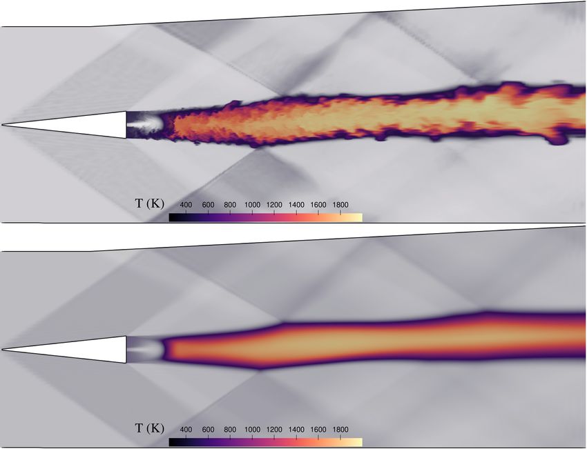
Figure 1. Schematic of the scramjet engine of a fictional hypersonic vehicle illustrating the combustor region considered in
this study.

    Due to the extreme flow environment, experimental measurements are difficult to be obtained and encompass many
uncertainties. Computational Aerospace Propulsion (CAP) provides a powerful framework for advancing the design and
development of scramjet engines. CAP can give insight into the details of the flow and chemistry in different parts of the
domain, can provide data for quantities that are limited by instrumentation, and can help repeat computations at a reduced cost
compared to ground test facilities. However, it also encompasses numerical and physics modelling challenges for supersonic
combustion. Ideally, one wants to reduce uncertainty by making simulations and experiments to converge to the same, or very
similar, answer.
    The recent development of very high-order methods for implicit large-eddy simulations (ILES) of supersonic and hypersonic
flows showed promising results12–14 . Therefore, in this study we employ high-order ILES, 11th-order accurate, to model and
simulate the scramjet supersonic combustion process. We aim at shedding light in the flow physics, e.g., by analysing the
Reynolds stress anisotropy to identify mechanisms influencing the combustion process and correlate the turbulent anisotropy
with the combustion chamber’s turbulent contraction and expansion, as well as hydroxyl (OH) production. We believe that
these processes could potentially be controlled to help make supersonic combustion more efficient.

3D Scramjet combustion
The flow configuration follows the experimental setup at DLR10 using a typical strut-based injection system in a supersonic
combustion ramjet. The side-view schematic of the scramjet combustion chamber is shown in Fig. 2. The preheated vitiated air
inlet of this combustor has a height of 50 mm and a width of 40 mm. The upper wall of the combustor has a divergence angle of
3° to compensate for the boundary-layer growth. The wedge is 32 mm long, and its half-angle is 6°. At the centre of the base of
the wedge, hydrogen at sonic condition (Mach 1) is injected into a Mach 2 supersonic preheated airflow through 15 holes of
diameter 1 mm and 2.4 mm apart. For the simulation presented here, three of the holes were simulated. The total length and
width of the computational zone are 340 mm and 7.2 mm, respectively. The flow conditions of the incoming vitiated air stream

and the hydrogen jet are given in Table 1. Note that the time-step size for the simulation was of the order of O 10−8 sec,
despite not resolving the viscous no-slip surfaces.
    Previous computational and experimental comparisons for the DLR supersonic combustion experiment show that the
experimental root mean square for the velocity is out of the free stream velocity range in some positions. In contrast,
computations4 are closer to the correct speed (about one dimensionless). This is evidence of the challenge of measuring in such
extreme flow conditions.

                                                                                                                          2/23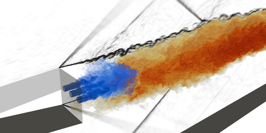
57mm                       3o

                                                             x=70mm                                x=117mm

                             25mm
                 Air                                        Fuel
                 M=2                12 o                    M=1
       50mm

                                           32mm

                              59mm

                                                                              172mm

Figure 2. Schematic of scramjet domain simulated overlayed with an illustration of the profiles location used in the
comparison; background plot of the mean temperature field given for illustration purposes.

                             Condition            Ma    p (bar)         T (K)     YO2      YN2       YH2 O     YH2

                                   Air            2         1           340      0.232    0.736      0.032      0
                              Fuel (H2 )          1         1           250        0           0          0     1

        Table 1. Inflow conditions of hydrogen fuel and atmospheric air for the DLR10 scramjet case configuration.

Computational methods accuracy
According to Fig. 3, the distance from the H2 jet exit outlet at which combustion is sustained is considerably further downstream
for both the 2nd - (M2LM) and 5th -order (M5LM) MUSCL limiters. Moreover, it was observed that without augmenting the
2nd -order MUSCL limiter with the low-Mach number correction (as per §), the flame would not be sustained and would
eventually extinguish. Although the flow is predominantly supersonic in the streamwise direction, applying the low-Mach
number correction reduces the numerical dissipation of the fluxes along the vertical path and the subsonic region behind the
wedge. The resulting enhanced turbulence that is resolved is more effective in mixing the air with the hydrogen fuel and
reducing the mean streamwise velocity.
     Arguably, the downstream position at which the flame initiates and is sustained is one of the most challenging and critical
flow properties necessary to be accurately captured. The experiment indicates –according to the temperature profiles in Figure 4
– that combustion initiates around x ≤ 70 mm. Since the 11th -order WENO scheme provided the most accurate result, as evident
in Fig. 3, all other schemes have been omitted in the subsequent analysis.
                                    ✁☛☛☛
                                    ✆☞✄☛
                                    ✆✄☛☛                                                            ✁✂
                                                                                                    ✄✂
                                     ✡ ✆✁✄☛                                                        ☎✆✆
                               ✝ ✠✟✞
                                       ✆☛☛☛
                                      ☞✄☛
                                      ✄☛☛
                                      ✁✄☛✑☛            ☞☛          ✒☛            ✓☛      ✆☛☛        ✆✆☛       ✆✁☛
                                                                              ✌ ✍✎✎✏
Figure 3. Comparison of mean temperature, T̃ , profiles along y = 0mm, starting from the centre of the H2 inlet jet at
x = 59mm and up to x = 117mm.

                                                                                                                            3/23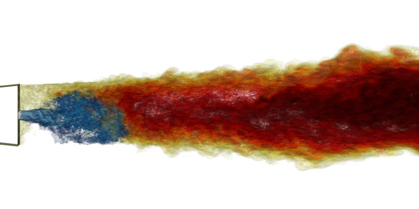
Computation vs experiment
We have first performed comparisons against the experimental results bearing in mind the uncertainties about experimental
measurements and matching the exact initial conditions between experiments and simulations.
    The mean axial velocity, hũx i, obtained using the high-order ILES, compares overall favourably to the experiment DLR10 at
two different locations, x = 70mm (upper graph) and x = 117mm (lower graph) (first column in Fig. 4). The experiment shows
a higher mean axial velocity in the vicinity of the hydrogen jet plum y/L = 0 for x = 70 mm, and slower at x = 117mm.

                                                                                                      1/2
Figure 4. Comparison of the mean axial velocity (hũi column 1), mean RMS axial velocity ( ug
                                                                                            ′′ u′′          column 2), mean
temperature ( T̃ column 3), profiles at different streamwise locations;
upper row x = 70mm, and lower row x = 117mm.

    The root-mean-square (RMS) profiles of the streamwise velocity fluctuations are shown in the second column of Fig. 4.
Above and below the mixing and combustion region, |y/L| > 0.1, the streamwise velocity RMS is smaller in the simulations
at both locations (x = 70mm & x = 117mm), suggesting either an issue with the calibration of the experimental measuring
devices or, more likely, the presence of significant velocity fluctuations in the incoming flow of the experiment. This result
suggests that either the inflow fluctuations upstream of the wedge or (and) the boundary layer characteristics in the inclined
surfaces of the strut/wedge and combustor walls are not accurately represented in the simulation as they were in the actual
experiment. The above is part of the uncertainty of validating such flows. Unless the experiment could measure and provide
such information, a mismatch in the comparisons should be expected. At x = 160mm, the predicted RMS agrees much better
with the experiment, particularly at the strut’s wake.
    The mean temperature, T̃ , is underpredicted in the simulation at x = 70mm, however, this is commonplace among
computational studies15–19 of the particular experiment10 . On the other hand, at x = 117mm, the mean temperature profile
compares favourably with that of the experiment. The agreement of the peak value, in particular, indicates that the thermo-
chemistry numerical solver can accurately model the heat released from the combustion of the injected hydrogen fuel with the
Oxygen in the free-stream air.
    The main conclusions from the mean flow comparisons between simulations and experiments are:

                                                                                                                          4/23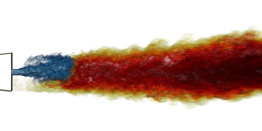
1. There is overall a good agreement between simulation and experiment.
2. The mean temperature profile at x = 117mm appears to diffuse more in the simulations than the experiment, i.e., in terms
of its shape (or distribution). However, the opposite is the case for the mean axial velocity and RMS.
3. At x = 70mm, the temperature in the strut’s wake is under-predicted while the mean axial velocity and RMS are
over-predicted.
The shape and dynamics of the recirculation bubbles that form in the strut’s wake may improve if the turbulent boundary
layer over the upper and lower inclined strut/wedge surfaces and the upper and lower shear layers formed just after the strut
corner edges are resolved. Therefore, an even better agreement between the experimental and numerical results may be
plausible. However, this would be at the expense of enormous computational cost due to the increase in the number of points
required to conduct wall-resolved simulations.
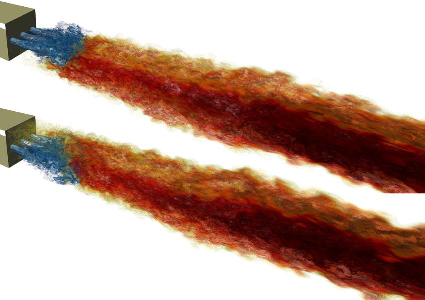
Figure 5. Illustration of an instantaneous snapshot of the three-dimensional flow; Blue: H2 fuel mass fraction
(YH2 = 0.4 − 1.0); Yellow-Orange: Temperature (T = 500 − 2000K); background contour plane of the density gradient
magnitude |∇ρ|.
Flow field structure
We present the 3D flow (Figure 5) using renderings of the instantaneous temperature, T , and hydrogen fuel mass-fraction,
YH2 , iso-surfaces, providing a qualitative understanding of the flow. The blue mist-like iso-surfaces signify a mass-fraction
of YH2 ≥ 0.5, while the solid iso-surface (mostly visible at the hydrogen fuel inlets) indicates a mass-fraction of YH2 = 1.
Regarding the flame, the yellow iso-surface indicates a temperature of 500K, while the darker orange has a temperature of
2, 000K. The high temperature is influenced by the two merging shockwaves at that location, as Fig. 2 suggests. The 3D
iso-surface image and the 2D contour plots show the short time and distance over which the ignition takes place, causing the
temperature to increase rapidly thereafter (Fig. 6). Temperatures as high as 2000 Kelvin are maintained for a long distance
downstream of the combustion onset (Fig. 6).
The simulation shows that the flame can propagate upstream towards the wedge, either from below or above the hydrogen
plume; the former being the case for the time instance depicted. This phenomenon is responsible for the prominent temperature
peaks at the edges of the strut’s wake observed in Fig. 4 for x = 70mm. Precisely, the entrainment of hydrogen fuel occurs along
the upper portion of the plume towards the strut due to a recirculation bubble in the strut’s wake (Fig. 5). The hydrogen becomes
trapped behind the strut until a sufficient amount of it is accumulated and eventually ignites with the aid of the downstream
flame.
5/23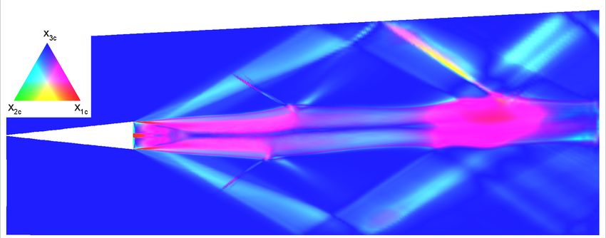
A closer inspection of the results reveals the flame moves upstream from above or below the hydrogen plume in an alternating
sequence. The enhanced mixing observed above and below the injected hydrogen plume causes the flame propagating upstream
and igniting the accumulated hydrogen once it has been sufficiently mixed – via turbulence transport – with Oxygen from
the freestream (atmospheric) air. Figure 5 clearly demonstrates the importance of the free shear layer in the mixing rate. The
mismatch of computations and experiments at the free shear layer (Fig. 4) could be due to the different resolved frequency
or duration of the alternating ignition sequence between the upper and lower free shear layers between experiments and
computations.
    Neglecting the viscous terms in such simulations subject to high accuracy in the advective terms with the optimal subgrid
dissipation for large-eddy simulations does not affect the mixing process between the hydrogen fuel and the atmospheric air in
the strut’s wake. Notably, the high-order WENO scheme maintained the flame at the correct distance from the strut/wedge as
indicated by the experiment, mainly thanks to its superior turbulence resolution. The above further supports that the advective
mixing due to the turbulence is dominant over molecular diffusion. Reducing the mismatch of the inflow conditions (velocity
perturbations) between experiments and simulations for the bulk flow turbulence intensity will undoubtedly help reduce the
prediction uncertainty. Furthermore, resolving the turbulent boundary layer over the strut’s surfaces at a more refined (grid-wise)
level could further increase the simulation accuracy in the vicinity of the free shear layer. However, this would severely increase
the computational cost.

Figure 6. Contour plot of an instantaneous 2D snapshot (upper) and the mean (lower) Temperature field in degrees Kelvin.

    Figure 6 shows the instantaneous (upper) and mean (lower) temperature fields. The instantaneous contour plot corresponds
to the spanwise mid-plane, right through the centre of the second H2 jet plume visible in Fig. 5.
    The combustion takes place just downstream of the H2 fuel plume breakdown. The upstream propagation of the flame along
the lower free shear layer observed in the instantaneous contour plot at a slightly lower temperature relative to the central flame
core, approximately 600 − 1500K, depending on the location and the stage of the “burst”. The mean Oxygen-to-Hydrogen
mass-fraction ratio in the wake of the strut is generally low, from below 1:10 in the mixing (or free shear) layer to nearly zero in
the mid-stream of the plume. Therefore, O2 alone cannot account for the consumption of the H2 fuel observed.
    For further clarity, we also provide the contour plot of the instantaneous and mean mass-fraction of the H2 fuel (Fig. 7)
as well as hydroxyl (Fig. 8). Particularly the latter component, OH, is an important transient species in Hydrogen-Oxygen

                                                                                                                               6/23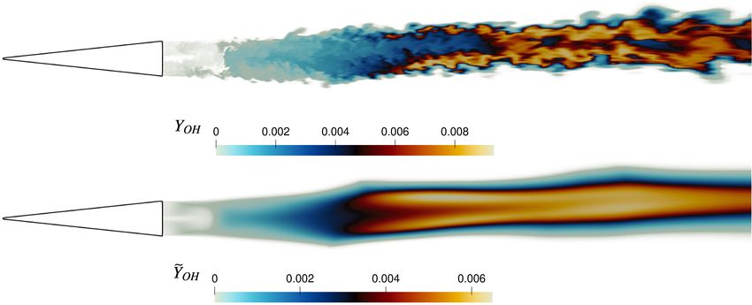
combustion. It contributes significantly to the rate of oxidation and heat release in low-temperature plasma thanks to the
relatively fast rate, at low temperature, of exothermic H abstraction by OH, such as the process OH+H2 ⇔ H+H2 O. It also has
a significant presence in the chain-branching reactions for a high-temperature combustion system.

              Figure 7. Contour plot of the instantaneous (upper) and the mean (lower) H2 fuel mass-fraction.

              Figure 8. Contour plot of the instantaneous (upper) and the mean (lower) OH fuel mass-fraction.

    Regarding the H2 fuel-injected, its rapid consumption at a short distance from the strut is evident. However, not all of the
H2 is consumed immediately, with a trace amount burnt gradually downstream of the flame front region. A gradual increase
in OH observed along the mixing layer downstream of the flame front appears to correlate well with the consumption of H2 ,
effectively splitting the latter into three streams of trace amounts. Importantly, this occurs at the region where the reflected
shocks –emanating from the strut’s leading-edge – converge into the flame’s outer area.
    At first glance, it appears as though the H2 fuel burns faster at the centre of the main flame front, rather than the outer regions
that are richer in O2 . However, this is caused by the recirculation bubbles in the strut’s wake and the gradual accumulation of
H2 . Specifically, the instantaneous plot of the H2 mass-fraction clearly shows a small amount released from behind the strut’s
upper wake region, along with its corresponding free shear layer. However, in the lower free shear layer, the H2 is consumed by
the flame propagating upstream towards the strut.
    The mean temperature and mass-fraction results in the vicinity of the strut’s wake and the flame front manifest the alternating
sequence of the upstream flame bursts between the lower and upper free shear layers.
    The temperature increases downstream – particularly along the flame’s inner core region – reaching a peak value of 2, 000K
despite the trace amounts of H2 . The culprit is predominantly the formation and consumption of OH, which is most abundant at
the same high-temperature regions. The gradual consumption of OH post both shock–flame interactions (that occur within the
computational domain extent employed) is evident and correlates well to the high-temperature regions. Note that the reflected

                                                                                                                                 7/23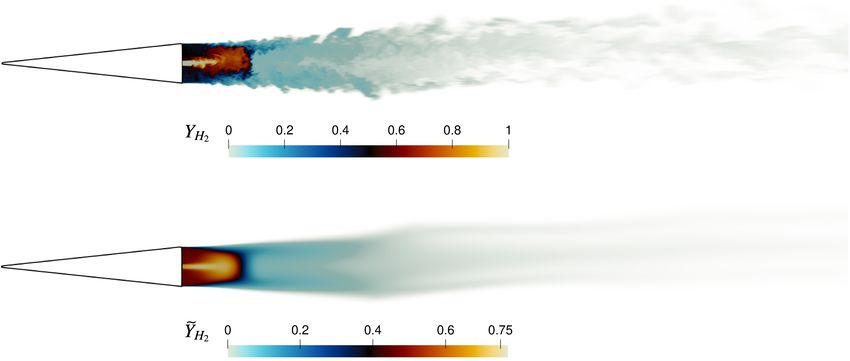
shock waves will also contribute directly to the temperature rise observed in the shock-flame interaction regions, but to a lesser
extent.
    The results demonstrate that there are two distinct central flame regions at the vicinity of the ignition front. First, the
“inner” region occurs where the main flame ignites as a result of the mixing between the H2 fuel plume and the atmospheric air
transported via the turbulent free shear layer. Second, the “outer” region occurs along (and just below) the upper and lower
turbulent free shear (or mixing) layers that form in the strut’s wake, where the concentration of O2 is the highest. However, the
two regions are not entirely distinct, and their dynamical behaviours are intertwined. When the flame propagates upstream and
the upper or lower mixing layers, the H2 jet plume is directed towards the other. As a result, a rich in H2 flow momentarily
forms at the inner flame’s front, causing it to move downstream. However, the H2 rich flow rapidly mixes with the turbulent free
shear layer, predominantly comprised of atmospheric air, and eventually forms a more favourable fuel-to-air ratio causing the
inner flame front to move back upstream again. The latter occurs while the flame initially propagates upstream, and the other
mixing layer begins to extinguish as the fuel-atmospheric air mix is consumed. Thus, the burnt fuel-air transports downstream
before the fuel-to-air ratio improves again and the process is repeated ad infinitum.

Turbulent free shear layer
Figures 9 and 10 depict 3D renderings of the instantaneous temperature, T , and hydrogen fuel mass-fraction, YH2 , iso-surfaces
at two different time instances, providing a qualitative understanding of the flow. More specifically, the blue iso-surface signifies
YH2 = 0.6, while the white iso-surface (mostly visible at the hydrogen fuel inlets) indicates YH2 = 1. Regarding the flame,
the yellow iso-surface indicates a temperature of 500K, while the dark-red has a temperature of 1, 900K. The latter is partly
attributed to the two merging shockwaves at that location, as Fig. 2 suggests. The 3D iso-surface images help illustrate how
short of a time and distance combustion takes place, causing the temperature to increase rapidly.

Figure 9. Iso-surfaces of H2 fuel (white-blue), and temperature (yellow-red-black) at two different time instances; isometric
view.

                                                                                                                                8/23
Figure 10. Iso-surfaces of H2 fuel mass-fraction (white-blue), and temperature (yellow-red-black) at two different time
instances; xy orthographic view.
Moreover, the 3D visualizations clearly show that the flame can propagate upstream towards the wedge below or above the
hydrogen plume. This phenomenon is responsible for the prominent temperature peaks at the edges of the strut’s wake that can
be seen in Fig. 4. More specifically, in Fig. 10, entrainment of hydrogen fuel can be seen moving along the upper portion of the
plume towards the strut due to a recirculation bubble in the strut’s wake. The hydrogen becomes trapped behind the strut until a
sufficient amount of it is accumulated that ignites the downstream flame.
A closer inspection of the computational data reveals that the flame moves upstream from above and below the hydrogen
plume in an alternating sequence. A possible explanation for the under-prediction of the temperature at the shear layer, as
indicated in Fig. 4, could be that the resolved frequency of the alternating sequence is lower than the experimental. Again,
the lack of resolving the turbulent boundary layer along the wedge and the subsequent shear layer is an attributing cause.
Furthermore, we should consider that the experiment also encompasses several uncertainties that deserve further investigation.
Figure 10 in particular, helps illustrate the importance that the under-resolved shear layer has on the flow evolution and
behaviour at this crucial region.
The temperature variation over time is extracted at two points, either one positioned between one of two free-shear layers
and the hydrogen plume, i.e., at (x, y) = (64, ±3) mm on the mid-plane (z = 3.6 mm). The signals’ power spectrum density
(PSD) is calculated and shown in Fig, 11. A peak at ≃ 7, 990 Hz is apparent, corresponding to the frequency at which the
free-shear layers periodically ignite, while the layers ignition is out of phase by 180°.
In conclusion, due to the very high Reynolds number of the case, neglecting the viscous terms did not adversely affect
the mixing processes between the hydrogen fuel and the atmospheric air in the strut’s wake. Notably, the high-order WENO
scheme maintained the flame at the correct distance from the strut/wedge as indicated by the experiment, mainly thanks to its
superior turbulence resolution. The above further supports that the advective mixing due to the turbulence is dominant over that
using molecular diffusion. Though considering the bulk flow turbulence and turbulent boundary layer could further increase the
simulation accuracy in the vicinity of the shear layer, this will be at the cost of severely increased computational demand.
9/23✘✓
✁✁✂✄
☎✆✝✂✄
✗
✌✒
✎ ✑✏ ✖
✍✡
☞✌☛
✡ ✕
✠
✟
✞
✔
✓
✘✓✓✓ ✘✓✪ ✘✓✫
✙✚✛✜✢✛✣✤✥ ✦✧★✩
Figure 11. Power spectrum density of temperature at just below the upper and lower turbulent free-shear layers; points
positioned on the mid-plane, z = 3.6 mm, at (x, y) = (64, ±3) mm.
Reynolds stress anisotropy
This study also sheds light on another aspect of flow physics. We have investigated the turbulence anisotropy using the
barycentric map method20 . We have implemented a modified map form to clarify the different turbulence anisotropy states21 . A
description of the procedure follows.
The Reynolds stress, Ri j , and the Reynolds stress anisotropy tensor, ai j , are calculated according to:
Ri j = ug
′′ u′′ = ρu′′ u′′ /ρ̄
i j i j (1)
and
Ri j δi j Rkk
ai j = − , where k =
2k 3 2
The three eigenvalues of the ai j (diagonal) tensor are obtained such that λ1 ≥ λ2 ≥ λ3 .
The eigenvalues are used to position the turbulence field on the barycentric anisotropy invariant map. The eigenvalues lie in
the interval −1/3 ≤ λi ≤ 2/3, and the number of non-zero eigenvalues and equalities between them identify the limiting states
of anisotropy. Based on their visual description, the limiting states are spherical, pancake-like and rod or cigar-like turbulence.
The first state corresponds to a three-component state, which is the isotropic turbulence, i.e., X3c (λ1 = λ2 = λ3 = 0). The
fluctuations are of equal magnitude and occur in all directions. Another state is the isotropic two-component turbulence X2c
(λ1 = λ2 = 1/6, λ3 = −1/3). In this case, fluctuations of equal magnitude occur in two directions. The last limiting state is
one-component turbulence X1c (λ1 = 2/3, λ2 = λ3 = −1/3), which describes a flow where turbulent fluctuations only exists
along one direction.
A convex combination of the above limiting states can describe any turbulence state. An equilateral triangle is constructed
to visualise the barycentric map. The peaks of the graph represent the limiting states (Fig. 12). Thus, we can identify both
the intensity and the type of turbulence anisotropy. A modified weights estimate is used to distinguish further the different
transition regions between the three limiting states of anisotropy:
Cexp
Xic = Cic +Co f f (2)
where
C1c = λ1 − λ2 , C2c = 2 (λ2 − λ3 ) , C3c = 3λ3 + 1
and Co f f = 0.65 and Cexp = 5.
The sides of the triangle (map boundaries) define the transition regions. The right side of the triangle, coloured magenta in
Fig. 12, corresponds to axisymmetric expansion in which one diagonal component of the Reynolds stress tensor is larger than
the other two, equal components. Thus, turbulence has a prolate spheroid shape. In the scramjet, the axisymmetric expansion is
the predominant turbulence anisotropy state in the strut’s wake and the flame region. It also occurs in the regions where (i)
10/23Figure 12. Contour plot of the Reynolds stress anisotropy componentality using Eq. (2) with Coff = 0.65 and Cexp = 5.
the strut’s leading-edge reflected shock waves from the walls interact with the flame; (ii) the H2 jet plume breaks down into
turbulence and undergoes mixing, and (iii) the turbulent free shear layers emanate from the corner edges of the wedge-shaped
strut.
In all of the above cases, the predominant Reynolds stress component of the axisymmetric expansion is the normal
streamwise component, R11 . Overall, the shock interactions and turbulent free shear layers make the turbulence state more
anisotropic. Note that the turbulence anisotropy state development of the turbulent free shear layers closely matches that
observed in non-reacting compressible but subsonic, free shear layers for a sudden-expansion geometry22 . However, the
axisymmetric turbulence state at the hydrogen’s plume mixing region transforms to an isotropic turbulence state at the flame’s
front. The sudden volumetric expansion that occurs as a result of the combustion initiation and rapid heating leads to a decrease
of the predominant incoming normal streamwise Reynolds stress component, R11 . The reduction is so pronounced that a steep
drop in the turbulence kinetic energy also occurs.
The left side of the triangle, coloured cyan, represents an axisymmetric contraction in which one component is smaller than
the other two parts, which are equal. The shape of turbulence is an oblate spheroid. The axisymmetric contraction of turbulence
is correlated mainly with the location of the expansion waves. Note that because no turbulence intensity was considered
in the upstream air in this study, turbulence fluctuations remained relatively weak upstream of the strut. Consequently, no
upstream nonlinear waves are visible in Fig. 12 –they are extremely steady. However, the two free shear layers that form at the
strut’s wake are both turbulent and the mixing that ensues downstream of the H2 injector outlets. The subsequent interaction
of the nonlinear waves with the strut’s turbulent wake induces to the former an unsteady motion, causing their appearance
on the anisotropy componentality map. Moreover, axisymmetric contraction can be observed along the region of hydroxyl
(OH) production Fig. 8, indicating that the chemical reactions processes here are likely different and, importantly, affect the
turbulence differently.
Another important observation is the “reaction” of turbulent flow to the second shock-flame interaction (Fig. 12). The
turbulence state in the entire surrounding region is transformed towards an axisymmetric expansion due to an increase in the
R11 component. Closer inspection shows that the increase occurs due to the turbulence flame interacting with the reflected
expansion waves rather than the reflected shock waves. The latter causes a decrease in R11 , such that a near isotropic turbulence
state occurs in the immediate vicinity downstream.
The two-component turbulence is shown at the bottom side of the triangle (in yellow). It can be visualised as an ellipse and
is typically present near the walls where the wall-normal component of the fluctuations vanishes much faster than the other
parts. The two-component turbulence also appears in the region of the reflected shock waves on the upper side of the domain. It
is caused by interacting with the reflected expansion waves.
Conclusions
The key findings from the present study are summarised below:
1. High-order simulations of supersonic combustion processes can shed light on the physics of the flow and combustion
that the experiment may not visualise and measure due to the extreme environment inside the scramjet. Specifically, the
11/23simulations show the fluid jets emanating from around the hydrogen plumes influencing the combustion process and the
high temperatures. Furthermore, the simulations provide information about turbulent anisotropy.
2. The shear layers above and below the fuel region are associated with strong turbulence anisotropy (axisymmetric
expansion).
3. The shock waves, reflecting from the wall and interacting with the flame, further result in a region of strong anisotropy.
4. The above event is also associated with hydroxyl production.
5. The highest mean temperature, T̃ , occurs shortly after the first shock-flame interaction, where an oval shaped region
between 1,840–1,880 K forms starting at (x, y) ≃ (98.5, 0.9) mm, ending at (x, y) ≃ (125, 2.1) mm, and of a maximum
thickness of ≈ 2.36 mm.
6. Small “pockets” of instantaneous temperature, T ≃ 1, 900 K occur within the region of the highest mean temperature,
T̃ . However, the highest instantaneous temperature range of 1,950–2000 K is found to be at the second shock-flame
interaction, i.e., (x, y) ≃ (134, 3.1)–(162, 4.8) mm, and of a maximum thickness of ≈ 7 mm.
7. The predictions show that the H2 fuel is consumed within a short distance from its injector outlets, approximately 13 mm.
8. The flame propagates upstream along with both turbulent free-shear layers at a frequency of ≃ 7, 990 Hz, while the two
are out of phase by 180°.
9. The computational and experimental results are within the same range and overall in good agreement. However, one
should consider that uncertainties arise from the mismatch of initial and boundary conditions between experiments and
simulations, e.g., the spanwise periodicity (3 holes vs 15), inlet condition (turbulence intensity), etc.
10. Resolving finer details of the corners around the scramjet edge and wall boundary layer would enable further physics
details. However, this would be at the expense of significantly higher computational costs. Furthermore, it remains to be
seen that such a demanding simulation would alter the above findings regarding the supersonic combustion processes.
We suggest that it is worth investigating the shear layers above and below the fuel plume and the shock/flame interaction,
particularly in the light of the turbulence anisotropy finding in these regions revealed in the present study.
Methods
Governing equations
Modelling detonation problems requires the use of the compressible Navier–Stokes equations in conjunction with complex
chemistry:
∂ρ
= −∇ · (ρu) (3)
∂t
∂ ρu
= −∇ · (ρu ⊗ u) − ∇p + ∇ · τ + ρb (4)
∂t
"N # Nsp
sp
∂ ρet
∂t
= − ∇ · (ρuht ) + ∇ · (u · τ) + ρu · b + ∇ · (k∇T ) + ∇ · ∑ (h j ρD j ∇Y j ) − ∑ (ρh j ω̇ j ) (5)
j=1 j=1
∂ ρY j
= −∇ · (ρY j u) + ∇ · (ρD j ∇Y j ) + ρ ω̇ j , (6)
∂t
where ht = et + p/ρ is hthe total specific enthalpy, k = c p µ/Pr th
i is the thermal conductivity, D j = µ j /(ρ Sc j ) is the j species
mass diffusivity, τ = µ ∇ ⊗ u + (∇ ⊗ u)T − (2/3) (∇ · u) I is the viscous stress tensor, µ is the dynamic viscosity, Pr and Sc
are the Prandtl and Schmidt numbers, respectively. No body forces have been considered in this study, i.e., b = 0. The energy
equation includes the inter-diffusional enthalpy flux arising from the species mixing23 . The species equations includes the rates
that account for the complex chemistry (combustion).
12/23Chemical reaction kinetics
Rates-of-change
Due to the chemical reaction(s), the individual species mass, as well as the mixture energy, will change. The chemical reactions
are summarised in Table 2. The following ODE describe the rates at which these take place:
dY j
(Y˙j ) ∼ = ω̇ j (7)
dt
˙ ∼ ρc p dT = − ρ
ρ (h)
dt ∑ M j j m, j ,
ω̇ H (8)
j
where Hm, j = h j /n j is the molar enthalpy of the jth species, while the specific enthalpy (per unit mass) is:
Hj Hj Hm, j
hj = = =
mj n jM j Mj
where n j = χ j n, and χ j is the molar-fraction of the jth species. The specific enthalpy is defined as h = ei + p/ρ = γei , where
ei = cv T = p/ [ρ (γ − 1)] is the specific internal energy; hence also h = c p T = γcv T ≡ γei . The molar mass of substance j is
defined as M j = m j /n j , therefore Eq. (8) can be written as:
sp N
dT
ρc p = − ∑ (ρ ω̇ j h j )
dt j
Note that the mass-fraction, Y j , and temperature, T , ODE required to be solved for complex chemistry are:
dY j
= ω̇ j (9)
dt
sp N
dT
cp = − ∑ (ω̇ j h j ) , (10)
dt j
where c p is the specific heat capacity at constant pressure of the mixture.
Progress rates
The mass reaction-rate of species j is the sum of all contributions from the elementary reactions:
M j Nre ′
ω̇ j = ∑ νi j − νi′′j ri (11)
ρ i=1
The progress rate ri of the i th reaction is defined as
Nsp Nsp
n′ n′′
ri = k f ,i ∏ c j i j − kr,i ∏ c j i j , (12)
j=1 j=1
where c j denotes the molar concentration of the species j, k f ,i and kr,i the forward and reverse constants of the i th reaction, and
exponents n′i j and n′′i j are equal to coefficients νi′j and νi′′j , respectively, if the i th reaction describes a true molecular process.
Note that νi′j and νi′′j are the stoichiometric coefficients of species j appearing as a reactant and as a product, respectively, in
reaction i.
Usually, the forward constants k f ,i are functions of temperature T and species concentrations c j . The particular expressions
for forward constant k f ,i are different for different chemical models. However, chemical models mostly used in combustion
share the same description of elementary chemical reactions, based on the modified Arrhenius law, leading to a rate coefficient
expressed as:
Ei
k f ,i = Ai T βi exp − (13)
Ru T
, with Ai the pre-exponential factor, βi the temperature exponent and Ei the activation energy of the i th reaction. The forward
and reverse constants of the reaction are linked by the equilibrium constant Ke,i :
k f ,i
Ke,i = (14)
kr,i
13/23that is expressed by:
Nsp
∑ νi′j − νi′′j
Patm j=1 ∆Sm,i ∆Hm,i
Ke,i = exp − (15)
Ru T Ru Ru T
The parameters ∆Sm,i and ∆Hm,i correspond to the ideal gas molar entropy and enthalpy change, respectively, during the
transition from reactants to products for the i th reaction. These quantities are obtained from tabulations based on experimental
measurements and/or theory.
For numerical simulations of reacting flows, a chemical scheme is required. Therefore, we must determine the knowledge
of all species and reactions before the computation can be carried out.
Thermodynamics
The non-dimensional heat capacities (determined experimentally or theoretically) are approximated with the temperature
polynomials given by
N
C pm, j
= ∑ an j T (n−1) , (16)
Ru n=1
where C pm, j is the molar heat capacity at constant pressure of the jth species. The approximation C pm, j (T ) is considered for
two temperature ranges and seven coefficients a j are needed for each of these ranges. According to Eq. (16), these polynomial
approximations take the following form:
C pm, j
= a1 j + a2 j T + a3 j T 2 + a4 j T 3 + a5 j T 4 , (17)
Ru
where the (absolute) temperature is in units of Kelvin.
Other ideal gas thermodynamic properties are given in terms of integrals of the C pm, j -function. First, the molar enthalpy is
defined by
ZT
◦
Hm, j = Hm, j (298K) + C pm, j dT, (18)
298K
so that
Hm, j N
an j T (n−1) aN+1, j
=∑ + , (19)
Ru T n=1 n T
where the parameter aN+1, j , represents the standard heat of formation at 298 K; the superscipt (◦ ) indicates conditions at a
Standard State, e.g., 1 atm, 298 K, pH 7.
The molar entropy is given by
ZT
◦ C pm, j
Sm, j = Sm, j (298K) + dT, (20)
T
298K
so that
Sm, j N
an j T (n−1)
= a1 j ln T + ∑ + aN+2, j , (21)
Ru n=2 (n − 1)
where the parameter aN+2, j , represents the standard entropy of formation at 298 K.
Hydrogen-Oxygen combustion
A total of 9 species (H2 , O2 , H2 O, O, H, OH, HO2 , H2 O2 , N2 ) and 20 chemical reactions are considered to model the combustion
process between the hydrogen fuel and atmospheric air (Table 1). The reduced model reaction set is given in Table 2 for
completeness.
The chemical reaction mechanism for hydrogen-oxygen shown in Table 2 is derived by reduction of a more extensive
mechanism24 . It has been validated using software tools for solving complex chemical kinetics problems, e.g. ChemKin,
including the burning temperature, ignition delay time, and species molar fractions.
14/23Reaction A B E
(1) H+O2 +M ⇔ HO2 +M 3.61E+17 -0.72 0.0
H2 O / 18.6 / H2 / 2.86 /
(2) 2H+M ⇔ H2 +M 1.0E+18 -1.0 0.0
(3) 2H+H2 ⇔ 2H2 9.2E+16 -0.6 0.0
(4) 2H+H2 O ⇔ H2 +H2 O 6.0E+19 -1.25 0.0
(5) H+OH+M ⇔ H2 O+M 1.6E+22 -2.0 0.0
H2 O / 5.0 /
(6) H+O+M ⇔ OH+M 6.2E+16 -0.6 0.0
H2 O / 5.0 /
(7) 2O+M ⇔ O2 +M 1.89E+13 0.0 -1788.0
(8) H2 O2 +M ⇔ 2OH+M 1.3E+17 0.0 45500.0
.
(9) H2 + O2 ⇔ 2OH 1.7E+13 0.0 47780.0
(10) OH+H2 ⇔ H2 O+H 1.17E+9 1.3 3626.0
(11) O+OH ⇔ O2 + H 3.61E+14 -0.5 0.0
(12) O+H2 ⇔ OH+H 5.06E+4 2.67 6290.0
(13) OH+HO2 ⇔ H2 O+O2 7.5E+12 0.0 0.0
(14) H+HO2 ⇔ 2OH 1.4E+14 0.0 1073.0
(15) O+HO2 ⇔ O2 +OH 1.4E+13 0.0 1073.0
(16) 2OH ⇔ O+H2 O 6.0E+8 1.3 0.0
(17) H+HO2 ⇔ H2 + O2 1.25E+13 0.0 0.0
(18) 2HO2 ⇔ H2 O2 +O2 2.0E+12 0.0 0.0
(19) H2 O2 +H ⇔ HO2 +H2 1.6E+12 0.0 3800.0
(20) H2 O2 +OH ⇔ H2 O+HO2 1.0E+13 0.0 1800.0
Table 2. Reduced chemical reaction mechanism (9 species and 20 reactions) used to model air-H2 combustion. The
pre-exponential factor (or frequency factor), A, has units of [s−1 ], the temperature dependency exponent, B, is dimensionless,
while the activation energy, E, is given here in [cal/mole].
ILES framework
The computational study is based on the CFD code CNS3D (Compressible Navier-Stokes Solver in 3D)25–27 . The code uses the
finite volume (upwind) Godunov method in conjunction with several approximate Riemann solvers, written in Fortran 2008. It
includes high-resolution methods of up to 11th -order of accuracy in space and 4th -order accuracy in time.
CNS3D can be used for implicit Large Eddy Simulations (iLES) and Direct Numerical Simulations (DNS)12, 28–30 . There
is also a Reynolds-Averaged Navier-Stokes (RANS) version of the code. The focus, however, of the present and future
developments is on iLES, which provide the best approach between accuracy and computational cost for any kind of engineering
geometry. In classical Large Eddy Simulations (LES), the smallest length scales, which are the most computationally expensive
to resolve, are removed via low-pass filtering of the Navier–Stokes equations. Then, the unresolved scales of turbulence are
modeled by subgrid-scale models. In iLES, the computational grid removes small scales. The modelling of the unresolved
scales is obtained through the non-linear dissipation embedded onto the high-resolution and high-order numerical schemes
used to discretize the convective terms. There is a significant body of work in the literature, both theoretical and numerical,
explaining iLES methods and demonstrating their accuracy in turbulent flows, e.g., see the books31, 32 .
In the present study, the HLLC solver is used in conjunction with a modified WENO 11th -order scheme12 . High-order
WENO schemes have proven resilient to the low-Mach number dissipation associated with compressible solvers33, 34 in
contrast to Monotonic Upstream-centered Scheme for Conservation Laws (MUSCL) type schemes35 , which generally require a
low-Mach number treatment such as that proposed by Thornber, Mosedale, Drikakis, Youngs and Williams36 (briefly described
in the following section).
Overview of numerical schemes
We employ the block-structured grid code CNS3D that solves the Navier–Stokes equations using the finite-volume method
(FVM). The advective terms are solved using the Godunov-type (upwind) method, whose inter-cell numerical fluxes are
calculated by solving the Riemann problem using the reconstructed values of the primitive variables at the cell interfaces. A
one-dimensional swept unidirectional stencil is used for spatial reconstruction. The variables reconstruction is carried out
accordingly37, 38 , to avoid spurious numerical oscillations from occurring at the interfaces between fluids of different heat
capacity ratios (γi 6= γ j ) due to the use of the four-equation model or otherwise the conservative mass-fraction transport equation
15/23(Eq. (6), diffuse-interface method)39 .
We have used a modified Weighted Essentially Non-Oscillatory (WENO) scheme, 11th order (W11), which we describe
below. We also use a second-order central scheme for the viscous terms. The solution is advanced in time using a five-stage
(fourth-order accurate) optimal strong-stability-preserving Runge–Kutta method40 . Further details about the code can be found
in Refs.12, 33, 34 and references therein.
Modified WENO Method
To address potential numerical instabilities due to the process of choosing an essentially non-oscillatory (ENO) stencil41 ,
Weighted ENO (WENO) methods were introduced42, 43 . WENO schemes use a convex combination of all the ENO candidate
stencils. Thus, the numerical flux is approximated by higher-order accuracy in smooth regions while still retaining the ENO
property in the flow regions near discontinuities; see44, 45 for an overview and further references. For WENO implementations
on structured grids, when the solution is locally smooth enough, the convex combination of the stencils of a rth -order ENO
scheme results in a (2r − 1)th -order WENO scheme42 .
Aiming to achieve a balance between accuracy and stability, we enhance the WENO schemes of 3rd and 5th -order of
Jiang and Shu43 (r = 2, 3) and 7th , 9th and 11th -order of Balsara and Shu46 (r = 4, 5, 6) by combining the mapped WENO
approach of Henrick, Aslam and Powers47 (WENO-M) and the relative total variation limiter approach of Taylor, Wu and
Martín48 (WENO-RLTV). WENO-M recovers the loss of accuracy occurring near smooth critical points. WENO-RLTV
reduces the numerical dissipation using the optimal linear weights in regions sufficiently smooth instead of the nonlinear
smoothness-indicator-based weights. The numerical reconstruction can be performed at the level of conservative, characteristic,
or primitive variables. The reconstruction of the conservative variables is more common in the literature. However, past research
has shown that such practice can lead to inaccuracies in capturing shock waves; see Zanotti and Dumbser49 and references
therein. Like other authors50 , we have opted to use the primitive variables in the high-order numerical reconstruction. The
characteristics-based variables would be more expensive computationally.
We present below a step-by-step description of the WENO procedure implemented to obtain the left reconstruction, qLi+1/2 ,
of the primitive variables, q = [ρ, u, p]T , at cell face i + 1/2:
1. The full (left and right reconstruction) stencil Si+1/2 G is normalized, per variable, according to the transformation
function:
G
Si+1/2 − gmin
Gz
Si+1/2 = (22)
gmax
where
G
Si+1/2 = (qi−r+1 , ... , qi+r )
and
G G
gmin = min Si+1/2 − 1, gmax = max Si+1/2 − qmin
while the new kth candidate stencil for the left reconstruction, containing r cell center values, is given by:
L Gz
Si+1/2;k = Si+1/2 [i − r + 1 + k, ... , i + k] ,
where k = 0, ... , r − 1. Eq. (22) simply normalizes the values of the candidate stencils prior to the estimation of the
smoothness indicators (IS) in such a way that (i) the maximum value of the full stencil becomes equal to one, i.e.,
Gz Gz
max(Si+1/2 ) = 1, (ii) the minimum value takes a positive and nonzero value, i.e. min(Si+1/2 ) > 0, and (iii) the value
range scales as originally relative to the maximum. By definition gmax is always positive and non-zero and hence Eq. (22)
will never result in an undefined operation and cause an exception. Using the above normalization of the full stencil
values, per variable, is found to (i) prevent negative WENO smoothness indicator values, (ii) reduce numerical dissipation,
and (iii) simplify the application of the proceeding step. The stencil normalization was found to have no effect on the
MUSCL-type slope limiters.
2. Next, a modified version of the relative total variation (TV) limiting procedure48 is implemented. The TV of each kth
candidate stencil is calculated according to:
r−1
TVk (Si;k ) = ∑ |qi−r+k+l+1 − qi−r+k+l | (23)
l=1
16/23Eq. (23) is then used to obtain the maximum TV ratio between the candidate stencils:
max (TVk )
R(TV) = (24)
min (TVk ) + ε
If all of the stencils contain significant discontinuities, then the value of R(TV) can be incorrectly small, i.e. R(TV) ≈ 1.
Thus, an additional criteria is introduced in order to avoid such a situation. The linear weights are used provided the
following two conditions are satisfied:
h
if R(TV) < ATV RL &
i
max (TVk ) < BTV then (25)
RL
ωkr = Ckr
According to Ref.48 , ATV TV
RL = 5, while for the second condition, BRL = 0.2(r − 1), where r is the order of the polynomials
used in the 2(r − 1) -order WENO. Note that the equation for BTV
th
RL is applicable only if the preceding pre-treatment/re-
scaling of the candidate stencils is carried out; otherwise it must be multiplied by qmax . In essence, the second condition
allows for an average TV of 20% between two neighbouring cells of the local stencils (SiG ) maximum variable value,
but this value can be modified if necessary. Wu and Martín51 used a value of BTV th
RL = 0.2 for their 4 -order bandwidth-
optimized WENO implementation in their DNS study.
Eq. (25) assumes that for the linear weights the condition ∑r−1 r
l=0 Cl = 1 is always satisfied.
3. If condition Eq. (25) is not satisfied, then the nonlinear weights based on the smoothness indicators of each candidate
stencil are computed according to the following two steps:
Ckr Ωrk
Ωrk = , ωkr = ,, (26)
(ISrk ) p + ε r−1 r
∑l=0 Ωl
where p = r and ε = 10−41 .
The standard WENO weights obtained in Eq. (26) are modified according to the mapped WENO (WENO-M) approach47
as:
Ω̃rk
ω̃kr = r−1 r
, (27)
∑l=0 Ω̃l
where, using the alternate formulation of Feng, Huang and Wang52 , the mapped weights are given by:
(Ωrk +Ckr )K+1 A
Ω̃rk = Ckr + (28)
(Ωk −Ckr )K A + Ωrk (1 − Ωrk )
r
and setting A = 1 and K = 2 results in the original mapping function47 .
4. The reconstructed scaled variable value at the left-side of cell-face i + 1/2 is given by:
r−1 h i
qLi+1/2 = ∑ ω̃kr f (q)rk , (29)
k=0
where
r−1
f (q)rk = ∑ αk;lr qi−r+k+l+1 (30)
l=0
5. Finally, due to the initial “normalizing” of the stencil in step 1, the reconstructed values obtained using Eq. (29) needs to
be “re-scaled” according to:
qLi+1/2 = qLi+1/2 gmax + gmin (31)
17/23WENO reconstruction can lead to spurious oscillations, if two or more shocks are too close to each other and WENO
cannot choose a single smooth stencil. To remedy this problem a procedure first introduced by Harten, Engquist, Osher and
Chakravarthy53 is adopted. If the reconstructed density and pressure values differ too drastically from their cell-center average
values, the order of the WENO reconstruction is reduced. After completion of the left and right reconstruction procedures at
cell-face i + 1/2, the left and right reconstructed density and pressure values are compared against their respective left and right
cell-center values:
L
ρi+1/2 − ρ i > C−
O or
(32)
R
ρi+1/2 − ρi+1 > C−
O
, where the order reduction threshold constant is set equal to C− O = 0.7. If the condition in Eq. (32) is met, then the order
of the WENO scheme is reduced according to (r − 1). The reconstruction procedure is then repeated for all variables, and
the condition is checked again. The process is repeated until Eq. (32) is not satisfied any longer. For example, assuming the
condition is repeatably met, a 9th -order WENO would first reduce to 7th -order, then to 5th , 3rd , and finally to the 2nd -order MC
MUSCL scheme. Titarev and Toro54 showed that the use of the above procedure does not degrade the high order of accuracy
for sufficiently smooth solutions.
As previously mentioned, for multi-component flows the following variables are reconstructed at the cell interfaces
q = [ρY j , u, p]T . However, WENO schemes do not adhere to the total variation diminishing (TVD) principle and are thus not
monotonicity preserving. Consequently, conservation of the species mass-fractions is not guaranteed and nonphysical values
can arise, i.e., negative or greater than one mass-fraction values. Therefore, following the WENO reconstruction of each j-th
species mass, ρY j , the obtained cell interface value is used to compute the equivalent MUSCL-scheme flux limiter, ψ ′ (ri )
according to:55 :
ψ ′ (ri ) = 2 qLi+1/2 − qi / (∆− )i (33)
where ri = ∆+ /∆− , ∆− = qi − qi−1 and ∆+ = qi+1 − qi . The equivalent flux limiter value is then “limited” such to remain
within the admissible limiter region for TVD schemes according to56 :
ψ (ri ) = max 0, min 2, 2r, ψ ′ (ri ) (34)
The final reconstructed cell interface value of the species mass is then obtained by substituting in Eq. (33) ψ ′ with ψ and
solving for qLi+1/2 .
Compressible filters
The accuracy of the present numerical schemes, and other methods, can be further enhanced in low-speed subsonic conditions by
implementing a low-Mach correction36 (henceforth labelled LMC). The low-Mach correction primarily involves an additional
computational step that treats the velocity vector via a progressive central differencing of its components. The LMC ensures
a balanced distribution of dissipation of kinetic energy in the limit of zero Mach number, thus extending the validity of
compressible flow codes to Mach numbers as low as 10−5 , and is mainly required for schemes providing accuracy less than
5th -order33, 34 .
After the reconstruction of the velocities has been carried out, the reconstructed left and right velocity components at
cell-face (i + 1/2) are modified according to:
uL,new
i+1/2 = (us − uu ) /2, uR,new
i+1/2 = (us + uu ) /2 (35)
where
us = uLi+1/2 + uRi+1/2 , uu = uLi+1/2 − uRi+1/2 Mmax (36)
L
and the maximum local Mach number is given by Mmax = max Mi+1/2 R
, Mi+1/2 .
Note that the density and pressure are not altered in any way during this step, thus the internal energy component
(ρe = p/(γ − 1)) remains unchanged. The reconstructed left and right total energies (et = e + ek ) are calculated using the
modified velocities in the kinetic energy component (ek = u · u/2).
18/23Details of the HLLC Riemann solver
The Riemann problem is solved here using the so-called “Harten, Lax, van Leer, and (the missing) Contact” (HLLC) approximate
Riemann solver of Toro, Bruce and Spears57 . More specifically, the adaptive non-iterative Riemann solver (ANRS) variant
proposed by Toro58 (see §9.5.2) is implemented. The following sequence details the approximate HLLC Riemann solver
procedure implemented:
1. To ensure high-order near the boundaries for high-order FVM codes, typically, the ghost-cell method is used to apply
the boundary conditions (BC). However, even after careful programming of the boundary conditions and reconstruction
procedures, computer rounding errors can persist and give rise to differences between the left and right reconstructed
states. Therefore, to ensure the appropriate flux, we modify the left and right reconstructed states for the following BCs:
symmetry plane (inviscid wall), heated (constant temperature) wall, and adiabatic (zero heat-flux) viscous (no-slip) wall.
For a symmetry plane, the no penetration condition is implemented for both advective and acoustic waves using the
procedure described by Algorithm 1.
if Left BC Viscous Wall then
pL = pR ;
if Wall Temperature then
if Left BC Symmetry then ρR = pR / (Rs TW );
ρL = ρR ; ρL = ρR ;
pL = pR ; uL = uR = 0;
uR = uR − (uR · n̂)uR ;
uL = uR ; else if Right BC Viscous Wall then
else if Right BC Symmetry then pR = pL ;
ρR = ρL ; if Wall Temperature then
pR = pL ; ρL = pL / (Rs TW );
uL = uL − (uL · n̂)uL ; ρR = ρL ;
uR = uL ; uL = uR = 0;
Algorithm 1: Ensure symmetry BC flux in HLLC.
Algorithm 2: Ensure viscous wall BC flux in
HLLC; if Wall Temperature true isothermal, else
adiabatic.
In the case of a viscous wall, Algorithm 2 is used instead. For an isothermal wall, the temperature at the ghost cells
is linearly interpolated from the interior domain and the wall. In this case, it is advisable to restrict the interpolated
temperature range of values to be only positive (T ∈ R>0 ), i.e. Tghosts > 10−15 , which reduces the likelihood of a
non-physical solution from manifesting.
2. An initial estimate of the pressure in the Star Region, that is the region defined in-between the two non-linear convective
wave-speeds (or characteristics), can be obtained according to59 :
p∗ = max 0, ppvrs (37)
which for curvilinear coordinates ppvrs is obtained according to:
1h i
ppvrs = pL + pR + u⊥ L − u⊥
R ρ̄ s̄
2 (38)
ρ̄ = (ρL + ρR ) /2 , s̄ = (sL + sR ) /2,
p
where the speed of sound is defined as s = γ p/ρ and u⊥ = u · n̂ is the magnitude of the velocity normal to the cell-face.
The “averaged” value of p∗ given by Eq. (37), is enhanced by taking into account the local conditions. The ANRS
approach58 introduces two conditions as a means to avoid unnecessary computations, i.e. updating the value of p∗
obtained by Eq. (37) with one that is more accurate. The first condition requires that the ratio between the maximum and
minimum local reconstructed pressures is greater than a predetermined constant, i.e.
Q = pmax /pmin > Quser ,
where pmin = min(pL , pR ), pmax = max(pL , pR ) and it is recommended that Quser = 2. The other condition requires that
p∗ does not lie between pmin and pmax , i.e. p∗ < pmin or p∗ > pmax . However, akin to non-differentiable (reconstruction)
19/23You can also read