INDIVIDUAL PRIVACY ACCOUNTING FOR DIFFEREN-TIALLY PRIVATE STOCHASTIC GRADIENT DESCENT
←
→
Page content transcription
If your browser does not render page correctly, please read the page content below
Under review as a conference paper at ICLR 2023

I NDIVIDUAL P RIVACY ACCOUNTING FOR D IFFEREN -
TIALLY P RIVATE S TOCHASTIC G RADIENT D ESCENT

 Anonymous authors
 Paper under double-blind review

                                               A BSTRACT
         Differentially private stochastic gradient descent (DP-SGD) is the workhorse al-
         gorithm for recent advances in private deep learning. It provides a single privacy
         guarantee to all datapoints in the dataset. We propose an efficient algorithm to
         compute privacy guarantees for individual examples when releasing models trained
         by DP-SGD. We use our algorithm to investigate individual privacy parameters
         across a number of datasets. We find that most examples enjoy stronger privacy
         guarantees than the worst-case bound. We further discover that the training loss
         and the privacy parameter of an example are well-correlated. This implies groups
         that are underserved in terms of model utility are simultaneously underserved in
         terms of privacy guarantee. For example, on CIFAR-10, the average ε of the class
         with the lowest test accuracy is 43.6% higher than that of the class with the highest
         accuracy.

1    I NTRODUCTION
Differential privacy is a strong notion of data privacy, enabling rich forms of privacy-preserving
data analysis (Dwork & Roth, 2014). Informally speaking, it quantitatively bounds the maximum
influence of any datapoint using a privacy parameter ε, where a small value of ε corresponds to
stronger privacy guarantees. Training deep models with differential privacy is an active research area
(Papernot et al., 2017; Bu et al., 2020; Yu et al., 2022; Anil et al., 2021; Li et al., 2022; Golatkar et al.,
2022; Mehta et al., 2022; De et al., 2022; Bu et al., 2022). Models trained with differential privacy
not only provide theoretical privacy guarantee to their data but also are more robust against empirical
attacks (Bernau et al., 2019; Carlini et al., 2019; Jagielski et al., 2020; Nasr et al., 2021).
Differentially private stochastic gradient descent (DP-SGD) is the de-facto choice for differentially
private deep learning (Song et al., 2013; Bassily et al., 2014; Abadi et al., 2016). DP-SGD first clips
individual gradients and then adds Gaussian noise to the average of clipped gradients. Standard
privacy accounting takes a worst-case approach, and provides all examples with the same privacy
parameter ε. However, from the perspective of machine learning, different examples can have very
different impacts on a learning algorithm (Koh & Liang, 2017; Feldman & Zhang, 2020). For
example, consider support vector machines: removing a non-support vector has no effect on the
resulting model, and hence that example would have perfect privacy.
In this paper, we give an efficient algorithm to accurately estimate individual privacy parameters of
models trained by DP-SGD. Our privacy guarantee adapts to the training trajectory of one execution
of DP-SGD to provide a precise characterization of privacy cost (see Section 2.1 for more details).
Inspecting individual privacy parameters allows us to better understand example-wise impacts. It
turns out that, for common benchmarks, many examples experience much stronger privacy guarantee
than the worst-case bound. To illustrate this, we plot the individual privacy parameters of MNIST
(LeCun et al., 1998), CIFAR-10 (Krizhevsky, 2009), and UTKFace (Zhang et al., 2017) in Figure 1.
Experimental details, as well as more results, can be found in Section 4 and 5. The disparity in
individual privacy guarantees naturally arises when running DP-SGD. To the best of our knowledge,
our investigation is the first to explicitly reveal such disparity.
We propose two techniques to make individual privacy accounting viable for DP-SGD. First, we
maintain estimates of the gradient norms for all examples so the individual privacy costs can be
computed accurately at every update. Second, we round the gradient norms with a small precision r
to control the number of different privacy costs, which need to be computed numerically. We explain

                                                      1
Under review as a conference paper at ICLR 2023

                               CIFAR-10, test acc.=74.2, max i=7.8, min i=1.1                  MNIST, test acc.=97.1, max i=2.4, min i=0.3
                          24000                                                          8000
                          22000                                                          7200
                          20000                                                          6400
                          18000
                          16000                                                          5600
                          14000                                                          4800

                  Count

                                                                                 Count
                          12000                                                          4000
                          10000                                                          3200
                           8000                                                          2400
                           6000
                           4000                                                          1600
                           2000                                                           800
                              0                                                             0
                               0.9 1.6 2.3 3.0 3.7 4.4 5.1 5.8 6.5 7.2 7.9                   0.1 0.3 0.5 0.7 0.9 1.1 1.3 1.5 1.7 1.9 2.1 2.3 2.5

                            UTKFace-Gender, test acc.=88.2, max i=4.5, min i=0.7            UTKFace-Age, test acc.=80.4, max i=4.2, min i=0.7
                           4000                                                          4000
                           3600                                                          3600
                           3200                                                          3200
                           2800                                                          2800
                           2400                                                          2400
                   Count

                                                                                 Count
                           2000                                                          2000
                           1600                                                          1600
                           1200                                                          1200
                            800                                                           800
                            400                                                           400
                              0                                                             0
                               0.5 0.9 1.3 1.7 2.1 2.5 2.9 3.3 3.7 4.1 4.5 4.9               0.5 0.9 1.3 1.7 2.1 2.5 2.9 3.3 3.7 4.1 4.5

Figure 1: Individual privacy parameters of models trained by DP-SGD. The value of δ is 1 × 10⁻⁵ .
The dashed lines indicate 10%, 30%, and 50% of datapoints. The black solid line shows the privacy
parameter of the original analysis.

why these two techniques are necessary in Section 2. More details of the proposed algorithm, as well
as methods to release individual privacy parameters, are in Section 3.

We further demonstrate a strong correlation between the privacy parameter of an example and its final
training loss. We find that examples with higher training loss also have higher privacy parameters in
general. This suggests that the same examples suffer a simultaneous unfairness in terms of worse
privacy and worse utility. While prior works have shown that underrepresented groups experience
worse utility (Buolamwini & Gebru, 2018), and that these disparities are amplified when models are
trained privately Bagdasaryan et al. (2019); Suriyakumar et al. (2021); Hansen et al. (2022); Noe
et al. (2022), we are the first to show that the privacy guarantee and utility are negatively impacted
concurrently. This is in comparison to prior work in the differentially private setting which took a
worst-case perspective for privacy accounting, resulting in a uniform privacy guarantee for all training
examples. For instance, when running gender classification on UTKFace, the average ε of the race
with the lowest test accuracy is 25% higher than that of the race with the highest accuracy. We also
study the disparity in privacy when models are trained without differential privacy, which may be of
independent interest to the community. We use the success rates of membership inference attacks to
measure privacy in this case and show groups with worse accuracy suffer from higher privacy risks.

1.1   R ELATED W ORK
Several works have explored example-wise privacy guarantees in differentially private learning.
Jorgensen et al. (2015) propose personalized differential privacy that provides pre-specified individual
privacy parameters which are independent of the learning algorithm, e.g., users can choose different
levels of privacy guarantees based on their sensitivities to privacy leakage (Mühl & Boenisch, 2022).
A recent line of works also uses the variation in example-wise sensitivities that naturally arise
in learning to study example-wise privacy. Per-instance differential privacy captures the privacy
parameter of a target example with respect to a fixed training set (Wang, 2019; Redberg & Wang,
2021; Golatkar et al., 2022). Feldman & Zrnic (2021) design an individual Rényi differential privacy
filter. The filter stops when the accumulated cost reaches a target budget that is defined before
training. It allows examples with smaller per-step privacy costs to run for more steps. The final
privacy guarantee offered by the filter is still the worst-case over all possible outputs as the predefined
budget has to be independent of the algorithm outcomes. In this work, we propose output-specific
differential privacy and give an efficient algorithm to compute individual guarantees of DP-SGD. We
further discover that the disparity in individual privacy parameters correlates well with the disparity
in utility.

                                                                                 2
Under review as a conference paper at ICLR 2023
2 P RELIMINARIES
We first give some background on differential privacy. Then we highlight the challenges in computing
individual privacy for DP-SGD. Finally, we argue that providing the same privacy bound to all
examples is not ideal because of the variation in individual gradient norms.
2.1 BACKGROUND ON D IFFERENTIALLY P RIVATE L EARNING
Differential privacy builds on the notion of neighboring datasets. A dataset D = {di }ni=1 is a
neighboring dataset of D′ (denoted as D ∼ D′ ) if D′ can be obtained by adding/removing one
example from D. The privacy guarantees in this work take the form of (ε, δ)-differential privacy.
Definition 1. [Individual (ε, δ)-DP] For a datapoint d, let D be an arbitrary dataset and D′ =
D ∪ {d} be its neighboring dataset. An algorithm A satisfies (ε(d), δ)-individual DP if for any
subset of outputs S ⊂ Range(A) it holds that
Pr[A(D) ∈ S] ≤ eε(d) Pr[A(D′ ) ∈ S] + δ and Pr[A(D′ ) ∈ S] ≤ eε(d) Pr[A(D) ∈ S] + δ.
We further allow the privacy parameter ε to be a function of a subset of outcomes to provide a sharper
characterization of privacy. We term this variant as output-specific (ε, δ)-DP. It shares similar insights
as the ex-post DP in Ligett et al. (2017); Redberg & Wang (2021) as both definitions tailor the privacy
guarantee to algorithm outcomes. Ex-post DP characterizes privacy after observing a particular
outcome. In contrast, the canonical (ε, δ)-DP is an ex-ante privacy notion. Ex-ante refers to ‘before
sampling from the distribution’. Ex-ante DP builds on property about the distribution of the outcome.
When the set A in Definition 2 contains more than one outcome, output-specific (ε, δ)-DP remains
ex-ante because it measures how the outcome is distributed over A.
Definition 2. [Output-specific individual (ε, δ)-DP] Fix a datapoint d and a set of outcomes A ⊂
Range(A), let D be an arbitrary dataset and D′ = D ∪ {d}. An algorithm A satisfies (ε(A, d), δ)-
output-specific individual DP for d at A if for any S ⊂ A it holds that
Pr[A(D) ∈ S] ≤ eε(A,d) Pr[A(D′ ) ∈ S] + δ and Pr[A(D′ ) ∈ S] ≤ eε(A,d) Pr[A(D) ∈ S] + δ.
Definition 2 has the same semantics as Definition 1 once the algorithm’s outcome belongs to A is
known. It is a strict generalization of (ε, δ)-DP as one can recover (ε, δ)-DP by maximizing ε(A, d)
over A and d. Making this generalization is crucial for us to precisely compute the privacy parameters
of models trained with DP-SGD. The output of DP-SGD is a sequence of models {θt }Tt=1 , where T is
number of iterations. The privacy risk at step t highly depends on the training trajectory (the first t − 1
models). For example, one can adversarially modify the training data and hence change the training
trajectory to maximize the privacy risk of a target example (Tramèr et al., 2022). With Definition 2,
we can analyze the privacy guarantee of DP-SGD with regards to a fixed training trajectory, which
specifies a subset of DP-SGD’s outcomes. In comparison, canonical DP analyzes the worst-case
privacy over all possible outcomes which could give loose privacy parameters.
A common approach for doing deep learning with differential privacy is to make each update
differentially private instead of protecting the trained model directly. The composition property
of differential privacy allows us to reason about the overall privacy of running several such steps.
We give a simple example
Pn to illustrate how to privatize each update. Suppose we take the sum of
all gradients v = i=1 gi from dataset D. Without loss of generality, further assume we add an
arbitrary example d′ to obtain a neighboring dataset D′ . The summed gradient becomes v ′ = v + g ′ ,
where g ′ is the gradient of d′ . If we add isotropic Gaussian noise with variance σ 2 , then the output
distributions of two neighboring datasets are
A(D) ∼ N (v, σ 2 I) and A(D′ ) ∼ N (v ′ , σ 2 I).
We then can bound the divergence between two Gaussian distributions to prove differential privacy,
e.g., through Rényi differential privacy (RDP) (Mironov, 2017). We give the definition of individual
RDP in Appendix A. The expectations of A(D) and A(D′ ) differ by g ′ . A larger gradient leads to a
larger difference and hence a worse privacy parameter.
2.2 C HALLENGES OF C OMPUTING I NDIVIDUAL P RIVACY PARAMETERS FOR DP-SGD
Privacy accounting in DP-SGD is more complex than the simple example in Section 2.1 because
the analysis involves privacy amplification by subsampling. Roughly speaking, randomly sampling
3Under review as a conference paper at ICLR 2023
a minibatch in DP-SGD strengthens the privacy guarantees since most points in the dataset are
not involved in a single step. How subsampling complicates the theoretical privacy analysis has
been studied extensively (Abadi et al., 2016; Balle et al., 2018; Mironov et al., 2019; Zhu & Wang,
2019; Wang et al., 2019). In this section, we focus on how subsampling complicates the empirical
computation of individual privacy parameters.
Before we expand on these difficulties, we first describe the output distributions of neighboring
datasets in DP-SGD (Abadi et al., 2016). Poisson
P sampling is assumed, i.e., each example is sampled
independently with probability p. Let v = i∈M gi be the sum of the minibatch of gradients of D,
where M is the set of sampled indices. Consider also a neighboring dataset D′ that has one datapoint
with gradient g ′ added. Because of Poisson sampling, the output is exactly v with probability 1 − p
(g ′ is not sampled) and is v ′ = v + g ′ with probability p (g ′ is sampled). Suppose we still add
isotropic Gaussian noise, the output distributions of two neighboring datasets are
A(D) ∼ N (v, σ 2 I), (1)
′ 2 ′ ′ 2
A(D ) ∼ N (v, σ I) with prob. 1 − p, A(D ) ∼ N (v , σ I) with prob. p. (2)
With Equation (1) and (2), we explain the challenges in computing individual privacy parameters.
2.2.1 F ULL BATCH G RADIENT N ORMS A RE R EQUIRED AT E VERY I TERATION
There is some privacy cost for d′ even if it is not sampled in the current iteration because the analysis
makes use of the subsampling process. For a given sampling probability and noise variance, the
amount of privacy cost is determined by ∥g ′ ∥. Therefore, we need accurate gradient norms of all
examples to compute accurate privacy costs at every iteration. However, when running SGD, we only
compute minibatch gradients. Previous analysis of DP-SGD evades this problem by simply assuming
all examples have the maximum possible norm, i.e., the clipping threshold.
2.2.2 C OMPUTATIONAL C OST OF I NDIVIDUAL P RIVACY PARAMETERS IS H UGE
The density function of A(D′ ) is a mixture of two Gaus-
sian distributions. Abadi et al. (2016) compute the Rényi DP-SGD on CIFAR-10 with = 7.5
divergence between A(D) and A(D′ ) numerically to get 25 Airplane
tight privacy parameters. Although there are some asymp- Automobile
Average Gradient Norm
totic bounds, those bounds are looser than numerical com- Cat
20
putation, and thus such numerical computations are nec-
essary in practice (Abadi et al., 2016; Wang et al., 2019; 15
Mironov et al., 2019; Gopi et al., 2021). In the classic
analysis, there is only one numerical computation as all 10
examples have the same privacy cost over all iterations.
However, naive computation of individual privacy param- 0 50 100 150 200
eters would require up to n × T numerical computations, Epoch
where n is the dataset size and T is the number of itera- Figure 2: Gradient norms on CIFAR-10.
tions.
2.3 A N O BSERVATION : G RADIENT N ORMS IN D EEP L EARNING VARY S IGNIFICANTLY
As shown in Equation 1 and 2, the privacy parameter of an example is determined by its gradient
norm once the noise variance is given. It is worth noting that examples with larger gradient norms
usually have higher training loss. This implies that the privacy cost of an example correlates with its
training loss, which we empirically demonstrate in Section 4 and 5. In this section, we show gradient
norms of different examples vary significantly to demonstrate that different examples experience very
different privacy costs. We train a ResNet-20 model with DP-SGD. The maximum clipping threshold
is the median of gradient norms at initialization. We plot the average norms of three different classes
in Figure 2. The gradient norms of different classes show significant stratification. Such stratification
naturally leads to different individual privacy costs. This suggests that quantifying individual privacy
parameters may be valuable despite the aforementioned challenges.
3 D EEP L EARNING WITH I NDIVIDUAL P RIVACY
We give an efficient algorithm (Algorithm 1) to estimate individual privacy parameters for DP-SGD.
The privacy analysis of Algorithm 1 is in Section 3.1. We perform two modifications to make
individual privacy accounting feasible with small computational overhead. First, we compute full
4Under review as a conference paper at ICLR 2023
batch gradient norms once in a while, e.g., at the beginning of every epoch, and use the results to
estimate the gradient norms for subsequent iterations. We show the estimations of gradient norms are
accurate in Section 3.2. Additionally, we round the gradient norms to a given precision so the number
of numerical computations is independent of the dataset size. More details of this modification are in
Section 3.3. Finally, we discuss how to make use of the individual privacy parameters in Section 3.4.
In Algorithm 1, we clip individual gradients with estimations of gradient norms (referred to as
individual clipping). This is different from the vanilla DP-SGD that uses the maximum threshold to
clip all examples (Abadi et al., 2016). Individual clipping gives us exact upper bounds on gradient
norms and hence we have exact bounds on privacy costs. Our analysis is also applicable to vanilla
DP-SGD though the privacy parameters in this case become estimates of exact guarantees, which is
inevitable because one can not have exact bounds on gradient norms at every iteration when running
vanilla SGD. We report the results for vanilla DP-SGD in Appendix C.2. Our observations include:
(1) the estimates of privacy guarantees for vanilla DP-SGD are very close to the exact ones, (2) all
our conclusions in the main text still hold when running vanilla DP-SGD, (3) the individual privacy
of Algorithm 1 is very close to that of vanilla DP-SGD.
Algorithm 1: Deep Learning with Individual Privacy Accounting
Input :Maximum clipping threshold C, rounding precision r, noise variance σ 2 , sampling probability p,
frequency of updating full gradient norms at every epoch K, number of epochs E.
1 Let {C (i) }n
i=1 be estimated gradient norms of all examples and initialize C
(i)
= C.
2 Let C = {r, 2r, 3r, . . . , C} be all possible norms under rounding.
3 for c ∈ C do
4 Compute Rényi divergences at different orders between Equation (1), (2) and store the results in ρc .
5 end
6 Let {o(i) = 0}n i=1 be the accumulated Rényi divergences at different orders.
7 for e = 1 to E do
8 for t′ = 1 to ⌊1/p⌋ do
9 t = t′ + ⌊1/p⌋ × (e − 1) //Global step count.
10 if t mod ⌊1/pK⌋ = 0 then
11 Compute full batch gradient norms {S (i) }n i=1 .
12 Update gradient estimates with rounded norms {C (i) = arg minc∈C (|c − S (i) |)}n
i=1 .
13 end
|I|
14 Sample a minibatch of gradients {g (Ij ) }j=1 , where I is the sampled indices.
(Ij ) (Ij ) (Ij )
15 Clip gradients ḡ = clip(g ,C ).
Update model θt = θt−1 − η( ḡ (Ij ) + z), where z ∼ N (0, σ 2 I).
P
16
17 for i = 1 to n do
18 Set ρ(i) = ρc where c = C (i) .
19 o(i) = o(i) + ρ(i) . //Update individual privacy costs.
20 end
21 end
22 end
3.1 P RIVACY A NALYSIS OF A LGORITHM 1
We state the privacy guarantee of Algorithm 1 in Theorem 3.1. We use output-specific DP to precisely
account the privacy costs of a realized run of Algorithm 1.
(i) log(1/δ)
Theorem 3.1. [Output-specific privacy guarantee] Algorithm 1 at step t satisfies (oα + α−1 , δ)-
(i)
output-specific individual DP for the ith example at A = (θ1 , . . . , θt−1 , Θt ), where oα is the
accumulated RDP at order α and Θt is the domain of θt .
To prove Theorem 3.1, we first define a t-step non-adaptive composition with θ1 , . . . , θt−1 . We then
show RDP of the non-adaptive composition gives an output-specific privacy bound on the adaptive
composition in Algorithm 1. We relegate the proof to Appendix A.
3.2 E STIMATIONS OF G RADIENT N ORMS A RE ACCURATE
Although the gradient norms used for privacy accounting are updated only occasionally, we show
that the individual privacy parameters based on estimations are very close to the those based on exact
5Under review as a conference paper at ICLR 2023
CIFAR-10: K = 0.5 MNIST: K = 0.5 UTKFace-Gender: K = 0.5 UTKFace-Age: K = 0.5
8 3 5 5
(estimated norms)
(estimated norms)
(estimated norms)
(estimated norms)
4 4
6
2 3 3
4 y=x y=x y=x y=x
2 2
y = 7.8 1 y = 2.4 y = 4.5 y = 4.2
2 Pearson's r = 0.999 Pearson's r = 0.996 1 Pearson's r = 0.992 1 Pearson's r = 0.991
Avg. | | = 0.06 Avg. | | = 0.06 Avg. | | = 0.09 Avg. | | = 0.08
Max | | = 0.39 Max | | = 0.22 Max | | = 0.37 Max | | = 0.35
00 2 4 6 8 00 1 2 3 00 2 4 00 2 4
(actual norms) (actual norms) (actual norms) (actual norms)
CIFAR-10: K = 1 MNIST: K = 1 UTKFace-Gender: K = 1 UTKFace-Age: K = 1
8 3 5 5
(estimated norms)
(estimated norms)
(estimated norms)
(estimated norms)
4 4
6
2 3 3
4 y=x y=x y=x y=x
2 2
y = 7.8 1 y = 2.4 y = 4.5 y = 4.2
2 Pearson's r = 1.000 Pearson's r = 0.998 1 Pearson's r = 0.999 1 Pearson's r = 0.997
Avg. | | = 0.04 Avg. | | = 0.04 Avg. | | = 0.05 Avg. | | = 0.06
Max | | = 0.25 Max | | = 0.16 Max | | = 0.32 Max | | = 0.31
00 2 4 6 8 00 1 2 3 00 2 4 00 2 4
(actual norms) (actual norms) (actual norms) (actual norms)
CIFAR-10: K = 3 MNIST: K = 3 UTKFace-Gender: K = 3 UTKFace-Age: K = 3
8 3 5 5
(estimated norms)
(estimated norms)
(estimated norms)
(estimated norms)
4 4
6
2 3 3
4 y=x y=x y=x y=x
2 2
y = 7.8 1 y = 2.3 y = 4.5 y = 4.2
2 Pearson's r = 1.000 Pearson's r = 0.994 1 Pearson's r = 1.000 1 Pearson's r = 1.000
Avg. | | = 0.02 Avg. | | = 0.08 Avg. | | = 0.01 Avg. | | = 0.01
Max | | = 0.20 Max | | = 0.21 Max | | = 0.07 Max | | = 0.08
00 2 4 6 8 00 1 2 3 00 2 4 00 2 4
(actual norms) (actual norms) (actual norms) (actual norms)
Figure 3: Privacy parameters based on estimations of gradient norms (ε) versus those based on exact
norms (έ). The results suggest that the estimations of gradient norms are close to the exact norms.
norms (Figure 3). This indicates that the estimations of gradient norms are close to the exact ones.
We comment that the privacy parameters computed with exact norms are not equivalent to those of
vanilla DP-SGD because individual clipping in Algorithm 1 slightly modifies the training trajectory.
We show individual clipping has a small influence on the individual privacy of vanilla DP-SGD in
Appendix C.2.
To compute the exact gradient norms, we randomly sample 1000 examples and compute the exact
gradient norms at every iteration. We compute the Pearson correlation coefficient between the privacy
parameters computed with estimated norms and those computed with exact norms. We also compute
the average and the worst absolute errors. We report results on MNIST, CIFAR-10, and UTKFace.
Details about the experiments are in Section 4. We plot the results in Figure 3. The ε values based on
estimations are close to those based on exact norms (Pearson’s r > 0.99) even we only update the
gradient norms every two epochs (K = 0.5). Updating full batch gradient norms more frequently
further improves the estimation, though doing so would increase the computational overhead.
It is worth noting that the maximum clipping threshold C affects the computed privacy parameters.
Large C increases the variation of gradient norms (and hence the variation of privacy parameters) but
leads to large noise variance while small C suppresses the variation and leads to large gradient bias.
Large noise variance and gradient bias are both harmful for learning (Chen et al., 2020; Song et al.,
2021). In Appendix D, we show the influence of using different C on both accuracy and privacy.
3.3 ROUNDING I NDIVIDUAL G RADIENT N ORMS
The rounding operation in Algorithm 1 is essential to make the computation of individual privacy
parameters feasible. The privacy cost of one example at each step is the Rényi divergences between
Equation (1) and (2). For a fixed sampling probability and noise variance, we use ρc to denote
the privacy cost of an example with gradient norm c. Note that ρc is different for every value of c.
Consequently, there are at most n × E different privacy costs because individual gradient norms
vary across different examples and epochs (n is the number of datapoints and E is the number of
training epochs). In order to make the number of different ρc tractable, we round individual gradient
norms with a prespecified precision r (see Line 12 in Algorithm 1). Because the maximum clipping
6Under review as a conference paper at ICLR 2023
threshold C is usually a small constant, then, by the pigeonhole principle, there are at most ⌈C/r⌉
different values of ρc . Throughout this paper we set r = 0.01C that has almost no impact on the
precision of privacy accounting.
Table 1: Computational costs of computing individual privacy parameters for CIFAR-10 with K = 1.
With Rounding Without Rounding
# of numerical computations 1 × 10² 1 × 10⁷
Time (in seconds)Under review as a conference paper at ICLR 2023
Figure 4: Privacy parameters and final training losses. Each point shows the loss and privacy
parameter of one example. Pearson’s r is computed between privacy parameters and log losses.
gradient norms at initialization, following the suggestion in Abadi et al. (2016). We set K = 3 for all
experiments in this section. More details about the hyperparameters are in Appendix B.
4.1 I NDIVIDUAL P RIVACY PARAMETERS VARY S IGNIFICANTLY
Figure 1 shows the individual privacy parameters on all datasets. The privacy parameters vary across
a large range on all tasks. On the CIFAR-10 dataset, the maximum εi value is 7.8 while the minimum
εi value is only 1.1. We also observe that, for easier tasks, more examples enjoy stronger privacy
guarantees. For example, ∼40% of examples reach the worst-case ε on CIFAR-10 while only ∼3%
do so on MNIST. This may because the loss decreases quickly when the task is easy, resulting in
gradient norms also decreasing and thus a reduced privacy loss.
4.2 P RIVACY PARAMETERS A ND L OSS A RE P OSITIVELY C ORRELATED
We study how individual privacy parameters correlate with individual training loss. The analysis in
Section 2 suggests that the privacy parameter of one example depends on its gradient norms across
training. Intuitively, an example would have high loss after training if its gradient norms are large. We
visualize individual privacy parameters and the final training loss values in Figure 4. The individual
privacy parameters on all datasets increase with loss until they reach the maximum ε. To quantify the
order of correlation, we further fit the points with one-dimensional logarithmic functions and compute
the Pearson correlation coefficients with the privacy parameters predicted by the fitted curves. The
Pearson correlation coefficients are larger than 0.9 on all datasets, showing an logarithmic correlation
between the privacy parameter of a datapoint and its training loss.
5 G ROUPS A RE S IMULTANEOUSLY U NDERSERVED IN B OTH ACCURACY AND
P RIVACY
5.1 L OW-ACCURACY G ROUPS H AVE W ORSE P RIVACY PARAMETERS
It is well-documented that machine learning models may have large differences in accuracy on
different groups (Buolamwini & Gebru, 2018; Bagdasaryan et al., 2019). Our finding demonstrates
that this disparity may be simultaneous in terms of both accuracy and privacy. We empirically verify
this by plotting the average ε and training/test accuracy of different groups. The experiment setup
is the same as Section 4. For CIFAR-10 and MNIST, the groups are the data from different classes,
while for UTKFace, the groups are the data from different races.
We plot the results in Figure 5. The groups are sorted based on the average ε. Both training and
test accuracy correlate well with ε. Groups with worse accuracy do have worse privacy guarantee
in general. On CIFAR-10, the average ε of the ‘Cat’ class (which has the worst test accuracy) is
43.6% higher than the average ε of the ‘Automobile’ class (which has the highest test accuracy). On
UTKFace-Gender, the average ε of the group with the lowest test accuracy (‘Asian’) is 25.0% higher
than the average ε of the group with the highest accuracy (‘Indian’). Similar observation also holds on
other tasks. To the best of our knowledge, our work is the first to reveal this simultaneous disparity.
5.2 L OW-ACCURACY G ROUPS S UFFER F ROM H IGHER E MPIRICAL P RIVACY R ISKS
We run membership inference (MI) attacks against models trained without differential privacy to
study whether underserved groups are more vulnerable to empirical privacy attacks. Several recent
works show that MI attacks have higher success rates on some examples than other examples (Song
8Under review as a conference paper at ICLR 2023
CIFAR-10 MNIST
Training Acc. (Max.-Min.=25.6%) 7.5 100 Training Acc. (Max.-Min.=3.8%)
Test Acc. (Max.-Min.=28.8%) Test Acc. (Max.-Min.=4.3%) 1.4
90 99
7.0 1.2
98
6.5
Accuracy (in %)
Accuracy (in %)
80 97 1.0
Average
Average
6.0 96 0.8
70 5.5 95 0.6
94
5.0 0.4
60
93
Privacy Parameter (Max.-Min.=2.39) 4.5 Privacy Parameter (Max.-Min.=0.43) 0.2
Ship Auto. Truck Frog Horse Air. Deer Dog Bird Cat 1 7 6 4 0 3 2 9 5 8
Subgroup Name Subgroup Name
UTKFace-Gender UTKFace-Age
3.2
100.0 Training Acc. (Max.-Min.=4.7%) Training Acc. (Max.-Min.=11.6%) 3.50
Test Acc. (Max.-Min.=5.8%) 3.0 Test Acc. (Max.-Min.=16.9%)
97.5 90 3.25
95.0 2.8
85 3.00
Accuracy (in %)
Accuracy (in %)
92.5 2.6
2.75
Average
Average
90.0 2.4 80
2.50
87.5 2.2 75 2.25
85.0 2.0
70 2.00
82.5
Privacy Parameter (Max.-Min.=0.54) 1.8 Privacy Parameter (Max.-Min.=0.97) 1.75
80.0
Indian Black White Asian Asian White Indian Black
Subgroup Name Subgroup Name
Figure 5: Accuracy and average ε of different groups. Groups with worse accuracy also have worse
privacy in general.
CIFAR-10 UTKFace-Gender UTKFace-Age
100 79.7 80 102.5 60.4 60.5 95 70.6
Test Accuracy Test Accuracy Test Accuracy
MI Success Rate MI Success Rate MI Success Rate 70
95 100.0 60.0
75 90
73.1 97.5 59.5 68
90
MI Success Rate
MI Success Rate
MI Success Rate
70.9 71.3 85
Test Accuracy
Test Accuracy
Test Accuracy
85 95.0 59.0 65.9 66
70
67.9 92.5 80
80 58.5
65.8 66.4 64
75 65 90.0 58.0
62.6 57.8 57.8 75 62.4
62
70 61.4 87.5 57.5
59.2 60 70
65 85.0 57.1 57.0
60.1 60
Auto. Ship TruckHorse Frog Air. Deer Dog Bird Cat Indian White Black Asian Asian White Indian Black
Subgroup Name Subgroup Name Subgroup Name
Figure 6: MI attack success rates on different groups. Target models are trained without DP
& Mittal, 2020; Choquette-Choo et al., 2021; Carlini et al., 2021). In this section, we directly connect
such disparity in privacy risks with the unfairness in utility. We use a simple loss-threshold attack that
predicts an example is a member if its loss value is smaller than a prespecified threshold (Sablayrolles
et al., 2019). For each group, we use its whole test set and a random subset of training set so the
numbers of training and test losses are balanced. We further split the data into two subsets evenly
to find the optimal threshold on one and report the success rate on another. More implementation
details are in Appendix B. The results are in Figure 6. The groups are sorted based on their average
ε. The disparity in privacy risks is clear. On UTKFace-Age, the MI success rate is 70.6% on the
‘Black’ group while is only 60.1% on the ‘Asian’ group. This suggests that empirical privacy risks
also correlate well with the disparity in utility.
6 C ONCLUSION
We propose an efficient algorithm to accurately estimate the individual privacy parameters for DP-
SGD. We use this new algorithm to examine individual privacy guarantees on several datasets.
Significantly, we find that groups with worse utility also suffer from worse privacy. This new
finding reveals the complex while interesting relation among utility, privacy, and fairness. It has two
immediate implications. Firstly, it shows that the learning objective aligns with privacy protection
for a given privacy budget, i.e., the better the model learns about an example, the better privacy
that example would get. Secondly, it suggests that mitigating the utility fairness under differential
privacy is more tricky than doing so in the non-private case. This is because classic methods such as
upweighting underserved examples would exacerbate the disparity in privacy.
9Under review as a conference paper at ICLR 2023
R EFERENCES
Martin Abadi, Andy Chu, Ian Goodfellow, H Brendan McMahan, Ilya Mironov, Kunal Talwar, and
Li Zhang. Deep learning with differential privacy. In Proceedings of ACM Conference on Computer
and Communications Security, 2016.
Galen Andrew, Om Thakkar, Brendan McMahan, and Swaroop Ramaswamy. Differentially private
learning with adaptive clipping. In Advances in Neural Information Processing Systems, 2021.
Rohan Anil, Badih Ghazi, Vineet Gupta, Ravi Kumar, and Pasin Manurangsi. Large-scale differen-
tially private BERT. arXiv preprint arXiv:2108.01624, 2021.
Eugene Bagdasaryan, Omid Poursaeed, and Vitaly Shmatikov. Differential privacy has disparate
impact on model accuracy. In Advances in Neural Information Processing Systems, 2019.
Borja Balle, Gilles Barthe, and Marco Gaboardi. Privacy amplification by subsampling: Tight
analyses via couplings and divergences. In Advances in Neural Information Processing Systems,
2018.
Raef Bassily, Adam Smith, and Abhradeep Thakurta. Private empirical risk minimization: Efficient
algorithms and tight error bounds. In Proceedings of the 55th Annual IEEE Symposium on
Foundations of Computer Science, 2014.
Daniel Bernau, Philip-William Grassal, Jonas Robl, and Florian Kerschbaum. Assessing differentially
private deep learning with membership inference. arXiv preprint arXiv:1912.11328, 2019.
Zhiqi Bu, Jinshuo Dong, Qi Long, and Weijie J. Su. Deep learning with Gaussian differential privacy.
Harvard Data Science Review, 2020.
Zhiqi Bu, Jialin Mao, and Shiyun Xu. Scalable and efficient training of large convolutional neural
networks with differential privacy. arXiv preprint arXiv:2205.10683, 2022.
Joy Buolamwini and Timnit Gebru. Gender shades: Intersectional accuracy disparities in commercial
gender classification. In Conference on Fairness, Accountability, and Transparency, 2018.
Nicholas Carlini, Chang Liu, Úlfar Erlingsson, Jernej Kos, and Dawn Song. The secret sharer:
Evaluating and testing unintended memorization in neural networks. In 28th USENIX Security
Symposium, 2019.
Nicholas Carlini, Steve Chien, Milad Nasr, Shuang Song, Andreas Terzis, and Florian Tramer.
Membership inference attacks from first principles. arXiv preprint arXiv:2112.03570, 2021.
Xiangyi Chen, Steven Z Wu, and Mingyi Hong. Understanding gradient clipping in private sgd: A
geometric perspective. Advances in Neural Information Processing Systems, 2020.
Christopher A Choquette-Choo, Florian Tramer, Nicholas Carlini, and Nicolas Papernot. Label-only
membership inference attacks. In Proceedings of the 38th International Conference on Machine
Learning, ICML ’21, pp. 1964–1974. JMLR, Inc., 2021.
Soham De, Leonard Berrada, Jamie Hayes, Samuel L Smith, and Borja Balle. Unlocking high-
accuracy differentially private image classification through scale. arXiv preprint arXiv:2204.13650,
2022.
Cynthia Dwork and Aaron Roth. The algorithmic foundations of differential privacy. Foundations
and Trends® in Theoretical Computer Science, 2014.
Vitaly Feldman and Chiyuan Zhang. What neural networks memorize and why: Discovering the long
tail via influence estimation. In Advances in Neural Information Processing Systems 33, 2020.
Vitaly Feldman and Tijana Zrnic. Individual privacy accounting via a Renyi filter. In Advances in
Neural Information Processing Systems, 2021.
Aditya Golatkar, Alessandro Achille, Yu-Xiang Wang, Aaron Roth, Michael Kearns, and Stefano
Soatto. Mixed differential privacy in computer vision. In Proceedings of IEEE Computer Society
Conference on Computer Vision and Pattern Recognition, 2022.
10Under review as a conference paper at ICLR 2023
Sivakanth Gopi, Yin Tat Lee, and Lukas Wutschitz. Numerical composition of differential privacy. In
Advances in Neural Information Processing Systems, 2021.
Victor Petrén Bach Hansen, Atula Tejaswi Neerkaje, Ramit Sawhney, Lucie Flek, and Anders Søgaard.
The impact of differential privacy on group disparity mitigation. arXiv preprint arXiv:2203.02745,
2022.
Kaiming He, Xiangyu Zhang, Shaoqing Ren, and Jian Sun. Deep residual learning for image
recognition. In Proceedings of IEEE Computer Society Conference on Computer Vision and
Pattern Recognition, 2016.
Matthew Jagielski, Jonathan Ullman, and Alina Oprea. Auditing differentially private machine
learning: How private is private sgd? In Advances in Neural Information Processing Systems,
2020.
Zach Jorgensen, Ting Yu, and Graham Cormode. Conservative or liberal? personalized differential
privacy. In International Conference on Data Engineering (ICDE), 2015.
Pang Wei Koh and Percy Liang. Understanding black-box predictions via influence functions. In
Proceedings of the 34th International Conference on Machine Learning, 2017.
Alex Krizhevsky. Learning multiple layers of features from tiny images, 2009.
Yann LeCun, Léon Bottou, Yoshua Bengio, and Patrick Haffner. Gradient-based learning applied to
document recognition. Proceedings of the IEEE, 1998.
Mathias Lécuyer. Practical privacy filters and odometers with rényi differential privacy and applica-
tions to differentially private deep learning. arXiv preprint arXiv:2103.01379, 2021.
Xuechen Li, Florian Tramèr, Percy Liang, and Tatsunori Hashimoto. Large language models can
be strong differentially private learners. In Proceedings of the 10th International Conference on
Learning Representations, 2022.
Katrina Ligett, Seth Neel, Aaron Roth, Bo Waggoner, and Steven Z Wu. Accuracy first: Selecting a
differential privacy level for accuracy constrained erm. Advances in Neural Information Processing
Systems, 2017.
Harsh Mehta, Abhradeep Thakurta, Alexey Kurakin, and Ashok Cutkosky. Large scale transfer
learning for differentially private image classification. arXiv preprint arXiv:, 2022.
Ilya Mironov. Rényi differential privacy. In Proceedings of the 30th IEEE Computer Security
Foundations Symposium, 2017.
Ilya Mironov, Kunal Talwar, and Li Zhang. Rényi differential privacy of the sampled gaussian
mechanism. arXiv preprint arXiv:1908.10530, 2019.
Christopher Mühl and Franziska Boenisch. Personalized PATE: Differential privacy for machine
learning with individual privacy guarantees. arXiv preprint arXiv:2202.10517, 2022.
Milad Nasr, Shuang Song, Abhradeep Thakurta, Nicolas Papernot, and Nicholas Carlini. Adver-
sary instantiation: Lower bounds for differentially private machine learning. arXiv preprint
arXiv:2101.04535, 2021.
Frederik Noe, Rasmus Herskind, and Anders Søgaard. Exploring the unfairness of dp-sgd across
settings. arXiv preprint arXiv:2202.12058, 2022.
Nicolas Papernot, Martín Abadi, Ulfar Erlingsson, Ian Goodfellow, and Kunal Talwar. Semi-
supervised knowledge transfer for deep learning from private training data. In Proceedings of the
5th International Conference on Learning Representations, 2017.
Rachel Redberg and Yu-Xiang Wang. Privately publishable per-instance privacy. In Advances in
Neural Information Processing Systems, 2021.
11Under review as a conference paper at ICLR 2023
Alexandre Sablayrolles, Matthijs Douze, Cordelia Schmid, Yann Ollivier, and Hervé Jégou. White-
box vs black-box: Bayes optimal strategies for membership inference. In Proceedings of the 36th
International Conference on Machine Learning, 2019.
Liwei Song and Prateek Mittal. Systematic evaluation of privacy risks of machine learning models.
arXiv preprint arXiv:2003.10595, 2020.
Shuang Song, Kamalika Chaudhuri, and Anand D Sarwate. Stochastic gradient descent with differ-
entially private updates. In Proceedings of IEEE Global Conference on Signal and Information
Processing, 2013.
Shuang Song, Thomas Steinke, Om Thakkar, and Abhradeep Thakurta. Evading the curse of
dimensionality in unconstrained private glms. In International Conference on Artificial Intelligence
and Statistics, 2021.
Vinith M Suriyakumar, Nicolas Papernot, Anna Goldenberg, and Marzyeh Ghassemi. Chasing
your long tails: Differentially private prediction in health care settings. In Proceedings of ACM
Conference on Fairness, Accountability, and Transparency, 2021.
Florian Tramèr, Reza Shokri, Ayrton San Joaquin, Hoang Le, Matthew Jagielski, Sanghyun Hong,
and Nicholas Carlini. Truth serum: Poisoning machine learning models to reveal their secrets.
arXiv preprint arXiv:2204.00032, 2022.
Yu-Xiang Wang. Per-instance differential privacy. The Journal of Privacy and Confidentiality, 2019.
Yu-Xiang Wang, Borja Balle, and Shiva Prasad Kasiviswanathan. Subsampled rényi differential
privacy and analytical moments accountant. In Proceedings of the 22nd International Conference
on Artificial Intelligence and Statistics, 2019.
Justin Whitehouse, Aaditya Ramdas, Ryan Rogers, and Zhiwei Steven Wu. Fully adaptive composi-
tion in differential privacy. arXiv preprint arXiv:2203.05481, 2022.
Ashkan Yousefpour, Igor Shilov, Alexandre Sablayrolles, Davide Testuggine, Karthik Prasad, Mani
Malek, John Nguyen, Sayan Ghosh, Akash Bharadwaj, Jessica Zhao, Graham Cormode, and
Ilya Mironov. Opacus: User-friendly differential privacy library in PyTorch. arXiv preprint
arXiv:2109.12298, 2021.
Da Yu, Saurabh Naik, Arturs Backurs, Sivakanth Gopi, Huseyin A Inan, Gautam Kamath, Janardhan
Kulkarni, Yin Tat Lee, Andre Manoel, Lukas Wutschitz, Sergey Yekhanin, and Huishuai Zhang.
Differentially private fine-tuning of language models. In Proceedings of the 10th International
Conference on Learning Representations, 2022.
Zhifei Zhang, Yang Song, and Hairong Qi. Age progression/regression by conditional adversarial
autoencoder. In Proceedings of IEEE Computer Society Conference on Computer Vision and
Pattern Recognition, 2017.
Yuqing Zhu and Yu-Xiang Wang. Poission subsampled Rényi differential privacy. In Proceedings of
the 36th International Conference on Machine Learning, 2019.
12Under review as a conference paper at ICLR 2023
A P ROOF OF T HEOREM 3.1
(i)
Theorem 3.1. [Output-specific privacy guarantee] Algorithm 1 at step t satisfies (oα + log(1/δ)
α−1 , δ)-
(i)
output-specific individual DP for the ith example at A = (θ1 , . . . , θt−1 , Θt ), where oα is the
accumulated RDP at order α and Θt is the domain of θt .
Here we give the the proof of Theorem 3.1. We compose the privacy costs at different steps through
Rényi differential privacy (RDP) (Mironov, 2017).RRDP uses the Rényi divergence at different orders
to measure privacy. We use Dα (µ||ν) = α−1 1
log ( dµ α
dν ) dν to denote the Rényi divergence at order
↔
α between µ and ν and Dα (µ||ν) = max(Dα (µ||ν), Dα (ν||µ)) to denote the maximum divergence
of two directions. The definition of individual RDP is as follows.
Definition 3. [Individual RDP Feldman & Zrnic (2021)] Fix a datapoint d, let D be an arbitrary
dataset and D′ = D ∪ {d}. A randomized algorithm A satisfies (α, ρ(d))-individual RDP for d if it
holds that Dα↔ (A(D)||A(D′ )) ≤ ρ(d).
Let (A1 , . . . , At−1 ) be a sequence of randomized algorithms and (θ1 , . . . , θt−1 ) be some arbitrary
fixed outcomes from the domain, we define
Â(t) (θ1 , . . . , θt−1 , D) = (A1 (D), A2 (θ1 , D), . . . , At (θ1 , . . . , θt−1 , D)).
Noting that Â(t) is not an adaptive composition as the input of each individual mechanism does not
depend on the outputs of previous mechanisms. Further let
A(t) (D) = (A1 (D), A2 (A1 (D), D), . . . , At (A1 (D), . . . , D))
be the adaptive composition. In Theorem A.1, we show a RDP bound on the non-adaptive composition
Â(t) gives an output-specific DP bound on the adaptive composition A(t) .
Theorem A.1. Let A = (θ1 , . . . , θt−1 , Range(At )) ⊂ Range(A(t) ) = Range(Â(t) ) where
θ1 , . . . , θt−1 are some arbitrary fixed outcomes. If Â(t) (·) satisfies oα RDP at order α, then A(t) (D)
satisfies (oα + log(1/δ)
α−1 , δ)-output-specific differential privacy at A.
Proof. For a given outcome θ(t) = (θ1 , θ2 , . . . , θt−1 , θt ) ∈ A, we have P A(t) (D) = θ(t) =
h i h i
P A(t−1) (D) = θ(t−1) P At (A1 (D), . . . , At−1 (D), D) = θt |A(t−1) (D) = θ(t−1) , (3)
h i
= P A(t−1) (D) = θ(t−1) P [At (θ1 , . . . , θt−1 , D) = θt ] , (4)
by the product rule of conditional
probability. Apply the product rule recurrently on
P A(t−1) (D) = θ(t−1) , we have P A(t) (D) = θ(t) =
h i
P A(t−2) (D) = θ(t−2) P [At−1 (θ1 , . . . , θt−2 , D) = θt−1 ] P [At (θ1 , . . . , θt−1 , D) = θt ] , (5)
= P [A1 (D) = θ1 ] P [A2 (θ1 , D) = θ2 ] . . . P [At (θ1 , . . . , θt−1 , D) = θt ] , (6)
h i
= P Â(t) (θ1 , . . . , θt−1 , D) = θ(t) . (7)
In words, A(t) and Â(t) are identical in A. Therefore, A(t) satisfies (ε, δ)-DP at any S ⊂ A if Â(t)
satisfies (ε, δ)-DP. Converting the RDP bound on Â(t) (D) into a (ε, δ)-DP bound with Lemma A.2
then completes the proof.
Lemma A.2 (Conversion from RDP to (ε, δ)-DP Mironov (2017)). If A satisfies (α, ρ)-RDP, then A
satisfies (ρ + log(1/δ)
α−1 , δ)-DP for all 0 < δ < 1.
13Under review as a conference paper at ICLR 2023
We comment that the RDP parameters of the adaptive composition of Algorithm 1 are random
variables because they depend on the randomness of the intermediate outcomes. This is different from
the conventional analysis that chooses a constant privacy parameter before training. Composition
of random RDP parameters requires additional care because one needs to upper bound the privacy
parameter over its randomness (Feldman & Zrnic, 2021; Lécuyer, 2021; Whitehouse et al., 2022). In
this paper, we focus on the realizations of those random RDP parameters and hence provide a precise
output-specific privacy bound.
B M ORE I MPLEMENTATION D ETAILS
The batchsize is 4K, 2K, and 200 for CIFAR-10, MNIST, and UTKFace, respectively. The training
epoch is 300 for CIFAR-10 and 100 for MNIST and UTKFace. We use the package in Yousefpour
et al. (2021) to compute the noise multiplier. The standard deviation of noise in Algorithm 1 is the
noise multiplier times the maximum clipping threshold. The non-private models in Section 5.2 are as
follows. For CIFAR-10, we use a ResNet20 model in He et al. (2016) that has ∼0.2M parameters,
with all batch normalization layers replaced by group normalization layers. For UTKFace, we use
the same models in Section 4. We remove both gradient clipping and noise for non-private training.
Other settings are the same as those in Section 4. All experiments are run on a single Tesla V100
GPU with 32G memory. Our source code, including the implementation of our algorithm as well as
scripts to reproduce the plots, will be released soon.
C M ORE D ISCUSSION ON I NDIVIDUAL C LIPPING
C.1 I NDIVIDUAL C LIPPING D OES N OT A FFECT ACCURACY
Here we run experiments to check the influence of using individual clipping thresholds on utility.
Algorithm 1 uses individual clipping thresholds to ensure the computed privacy parameters are strict
privacy guarantees. If the clipping thresholds are close to the actual gradient norms, then the clipped
results are close to those of using a single maximum clipping threshold. However, if the estimations
of gradient norms are not accurate, individual thresholds would clip more signal than using a single
maximum threshold.
Table 2: Comparison between the test accuracy of using individual clipping thresholds and that of
using a single maximum clipping threshold. The maximum ε is 7.8 for CIFAR-10 and 2.4 for MNIST.
CIFAR-10 MNIST
Individual 74.0 (±0.19) 97.17 (±0.12)
Maximum 74.1 (±0.24) 97.26 (±0.11)
We compare the accuracy of two different clipping methods in Table 2. The individual clipping
thresholds are updated once per epoch. We repeat the experiment four times with different random
seeds. Other setups are the same as those in Section 4. The results suggest that using individual
clipping thresholds in Algorithm 1 has a negligible effect on accuracy.
C.2 E XPERIMENTS W ITHOUT I NDIVIDUAL C LIPPING
We run Algorithm 1 without individual clipping, i.e., vanilla DP-SGD in Abadi et al. (2016), to see
whether our conclusions in the main text still hold. Specifically, we change the Line 15 of Algorithm 1
to clip all gradients with the maximum clipping threshold C. Other experimental setup is the same as
that in Experiment 4 and Appendix B.
We get accurate estimations of actual guarantees. The privacy parameters are still computed with
the estimations of gradient norms and hence are estimations of the actual guarantees. We compare
the privacy parameters and actual guarantees in Figure 7. To compute the actual guarantees, we
randomly sample 1000 examples and compute their exact gradient norms at every iteration. The
results suggest that the privacy parameters are accurate estimations (Pearson’s r > 0.99 and small
maximum absolute errors).
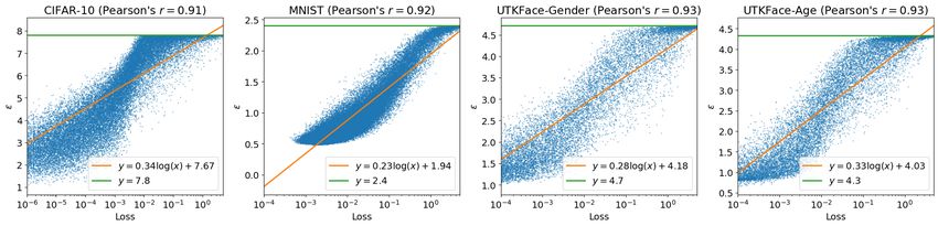
Privacy parameters still have a strong correlation with training loss. In Figure 8, we show
privacy parameters computed without individual clipping are still positively correlated with training
losses. The Pearson correlation coefficient between privacy parameters and log losses is larger than
14Under review as a conference paper at ICLR 2023
CIFAR-10: K = 0.5 MNIST: K = 0.5 UTKFace-Gender: K = 0.5 UTKFace-Age: K = 0.5
8 3 5 5
(estimated norms)
(estimated norms)
(estimated norms)
(estimated norms)
4 4
6
2 3 3
4 y=x y=x y=x y=x
2 2
y = 7.8 1 y = 2.4 y = 4.5 y = 4.2
2 Pearson's r = 0.998 Pearson's r = 0.995 1 Pearson's r = 0.999 1 Pearson's r = 0.999
Avg. | | = 0.09 Avg. | | = 0.07 Avg. | | = 0.05 Avg. | | = 0.05
Max | | = 0.54 Max | | = 0.25 Max | | = 0.35 Max | | = 0.29
00 2 4 6 8 00 1 2 3 00 2 4 00 2 4
(actual norms) (actual norms) (actual norms) (actual norms)
CIFAR-10: K = 1 MNIST: K = 1 UTKFace-Gender: K = 1 UTKFace-Age: K = 1
8 3 5 5
(estimated norms)
(estimated norms)
(estimated norms)
(estimated norms)
4 4
6
2 3 3
4 y=x y=x y=x y=x
2 2
y = 7.8 1 y = 2.4 y = 4.5 y = 4.2
2 Pearson's r = 0.999 Pearson's r = 0.998 1 Pearson's r = 1.000 1 Pearson's r = 1.000
Avg. | | = 0.06 Avg. | | = 0.04 Avg. | | = 0.02 Avg. | | = 0.02
Max | | = 0.35 Max | | = 0.17 Max | | = 0.14 Max | | = 0.19
00 2 4 6 8 00 1 2 3 00 2 4 00 2 4
(actual norms) (actual norms) (actual norms) (actual norms)
CIFAR-10: K = 3 MNIST: K = 3 UTKFace-Gender: K = 3 UTKFace-Age: K = 3
8 3 5 5
(estimated norms)
(estimated norms)
(estimated norms)
(estimated norms)
4 4
6
2 3 3
4 y=x y=x y=x y=x
2 2
y = 7.8 1 y = 2.3 y = 4.5 y = 4.2
2 Pearson's r = 1.000 Pearson's r = 0.999 1 Pearson's r = 1.000 1 Pearson's r = 1.000
Avg. | | = 0.04 Avg. | | = 0.01 Avg. | | = 0.01 Avg. | | = 0.01
Max | | = 0.32 Max | | = 0.07 Max | | = 0.06 Max | | = 0.17
00 2 4 6 8 00 1 2 3 00 2 4 00 2 4
(actual norms) (actual norms) (actual norms) (actual norms)
Figure 7: Privacy parameters based on estimations of gradient norms (ε) versus the actual privacy
guarantees (έ). We do not use individual clipping in this plot. The privacy parameters are very close
to the actual guarantees.
Figure 8: Privacy parameters and final training losses. The experiments are run without individual
clipping. The Pearson correlation coefficient is computed between privacy parameters and log losses.
0.9 for all datasets. Moreover, we show our observation in Section 5, i.e., low-accuracy groups have
worse privacy parameters, still holds in Figure 9. We also make a direct comparison with privacy
parameters computed with individual clipping. We find that privacy parameters computed with
individual clipping are very close to those computed without individual clipping. We also find that
the order of groups, sorted by the average ε, is exactly the same for both cases.
D T HE I NFLUENCE OF M AXIMUM C LIPPING ON I NDIVIDUAL P RIVACY
The value of the maximum clipping threshold C would affect individual privacy parameters. A large
value of C would increase the stratification in gradient norms but also increase the noise variance
for a fixed privacy budget. A small value of C would suppress the stratification but also increase the
gradient bias. Here we run experiments with different values of C on CIFAR-10. We use a ResNet20
for CIFAR-10 in He et al. (2016), which only has ∼0.2M parameters, to reduce the computation
cost. All batch normalization layers are replaced with group normalization layers. Let M be the
median of gradient norms at initialization, we choose C from the list [0.1M, 0.3M, 0.5M, 1.5M ].
Other experimental setup is the same as that in Section 4.
15Under review as a conference paper at ICLR 2023
100
CIFAR-10 MNIST
Test Acc. (Without I.C.) 100 Test Acc. (Without I.C.)
7.5 1.4
99
90 7.0 1.2
98
6.5 1.0
Accuracy (in %)
Accuracy (in %)
80 97
Average
Average
6.0 96 0.8
70 5.5 95 0.6
5.0 94 0.4
60 Privacy Parameter (Without I.C.) 93 Privacy Parameter (Without I.C.)
Privacy Parameter (With I.C.) Privacy Parameter (With I.C.) 0.2
4.5
Ship Auto. Truck Frog Horse Air. Deer Dog Bird Cat 1 7 6 4 0 3 2 9 5 8
Subgroup Name Subgroup Name
UTKFace-Gender 95
UTKFace-Age
100.0 Test Acc. (Without I.C.) 3.2 Test Acc. (Without I.C.) 3.50
97.5 3.0 90 3.25
95.0 2.8 3.00
85
Accuracy (in %)
Accuracy (in %)
92.5 2.6
Average 2.75
Average
90.0 2.4 80
2.50
87.5 2.2 75 2.25
85.0 2.0 2.00
82.5 70
Privacy Parameter (Without I.C.) 1.8 Privacy Parameter (Without I.C.)
Privacy Parameter (With I.C.) Privacy Parameter (With I.C.) 1.75
80.0 65
Indian Black White Asian Asian White Indian Black
Subgroup Name Subgroup Name
Figure 9: Test accuracy and privacy parameters computed with/without individual clipping (I.C.).
Groups with worse test accuracy also have worse privacy in general.
C=0.1M, test acc.=60.7, max i=7.5, min i=1.6 C=0.3M, test acc.=64.9, max i=7.5, min i=1.0
40000 35000
36000 31500
32000 28000
28000 24500
24000 21000
Count
Count
20000 17500
16000 14000
12000 10500
8000 7000
4000 3500
0 0
0.0 0.8 1.6 2.4 3.2 4.0 4.8 5.6 6.4 7.2 8.0 0.0 0.8 1.6 2.4 3.2 4.0 4.8 5.6 6.4 7.2 8.0
C=0.5M, test acc.=65.6, max i=7.5, min i=0.9 C=1.5M, test acc.=63.2, max i=7.5, min i=0.5
30000 10000
27000 9000
24000 8000
21000 7000
18000 6000
Count
Count
15000 5000
12000 4000
9000 3000
6000 2000
3000 1000
0 0
0.0 0.8 1.6 2.4 3.2 4.0 4.8 5.6 6.4 7.2 8.0 0.0 0.8 1.6 2.4 3.2 4.0 4.8 5.6 6.4 7.2 8.0
Figure 10: Distributions of individual privacy parameters on CIFAR-10 with different maximum
clipping thresholds. The dashed line indicates the average of privacy parameters.
16Under review as a conference paper at ICLR 2023
Clip=0.1 Median Clip=0.3 Median
8.0 90 8.0
Training Acc. (Max.-Min.=34.7%) Training Acc. (Max.-Min.=40.7%)
Test Acc. (Max.-Min.=34.3%) Test Acc. (Max.-Min.=41.0%)
80 7.5
7.5 80
70 7.0
Accuracy (in %)
Accuracy (in %)
70
7.0
Average
Average
60 60 6.5
6.5
6.0
50 50
6.0 5.5
Privacy Parameter (Max-Min=1.33) 40 Privacy Parameter (Max-Min=1.78)
40
Ship Frog Auto. Truck Air. Horse Dog Bird Deer Cat Ship Auto. Frog TruckHorse Air. Dog Bird Deer Cat
Subgroup Name Subgroup Name
Clip=0.5 Median Clip=1.5 Median
90 Training Acc. (Max.-Min.=35.5%) Training Acc. (Max.-Min.=33.9%) 5.50
Test Acc. (Max.-Min.=36.5%) 7.5 Test Acc. (Max.-Min.=33.6%)
80 5.25
80
7.0 5.00
Accuracy (in %)
Accuracy (in %)
70
70 4.75
Average
Average
6.5
60 4.50
60
6.0
4.25
50 50
5.5 4.00
Privacy Parameter (Max-Min=1.87) Privacy Parameter (Max-Min=0.91)
3.75
Ship Auto. Truck Frog Horse Air. Dog Bird Deer Cat Ship Auto. Truck Air. Frog Dog Horse Cat Deer Bird
Subgroup Name Subgroup Name
Figure 11: Accuracy and average ε of different groups on CIFAR-10 with different maximum clipping
thresholds.
The histograms of individual privacy parameters are in Figure 10. In terms of accuracy, using clipping
thresholds near the median gives better test accuracy. In terms of privacy, using smaller clipping
thresholds increases privacy parameters in general. The number of datapoints that reaches the worst
privacy decreases with the value of C. When C = 0.1M , nearly 70% datapoints reach the worst
privacy parameter while only ∼2% datapoints reach the worst parameter when C = 1.5M .
The correlation between accuracy and privacy is in Figure 11. The disparity in average ε is clear for
all choices of C. Another important observation is that when decreasing C, the privacy parameters of
underserved groups increase quicker than other groups. When changing C = 1.5M to 0.5M , the
average ε of ‘Cat’ increases from 4.8 to 7.4, almost reaching the worst-case bound. In comparison,
the increment in ε of the ‘Ship’ class is only 1.3 (from 4.2 to 5.5).
E M AKE U SE OF I NDIVIDUAL P RIVACY PARAMETERS
E.1 R ELEASING I NDIVIDUAL P RIVACY PARAMETERS TO R IGHTFUL OWNERS
Let εi be the privacy parameter of the ith user, we can compute εi with the training trajectory and di
itself. Theorem E.1 shows that releasing εi does not increase the privacy cost of any other example
dj ̸= di . The proof uses the fact that computing εi can be seen as a post-processing of (θ1 , . . . , θt−1 ),
which is reported in a privacy-preserving manner.
Theorem E.1. Let A : D → O be an algorithm that is (εj , δ)-output-specific DP for dj at A ⊂ O.
Let f (·, di ) : O → R × O be a post-processing function that returns the privacy parameter of di
(̸= dj ) and the training trajectory. We have f is (εj , δ)-output-specific DP for dj at F ⊂ R × O
where F = {f (a, di ) : a ∈ A} is all possible post-processing results.
Proof. We first note that the construction of f is independent of dj . Without loss of generality, let
D, D′ ∈ D be the neighboring datasets where D′ = D ∪ {dj }. Let S ⊂ F be an arbitrary event and
17You can also read