In vivo electrical conductivity measurement of muscle, cartilage, and peripheral nerve around knee joint using MR electrical properties tomography ...
←
→
Page content transcription
If your browser does not render page correctly, please read the page content below
www.nature.com/scientificreports

                OPEN             In vivo electrical conductivity
                                 measurement of muscle, cartilage,
                                 and peripheral nerve around knee
                                 joint using MR‑electrical properties
                                 tomography
                                 Ji Hyun Lee1, Young Cheol Yoon1*, Hyun Su Kim1, Jiyeong Lee1, Eunju Kim2,
                                 Christian Findeklee3 & Ulrich Katscher3

                                 This study aimed to investigate whether in vivo MR-electrical properties tomography (MR-EPT) is
                                 feasible in musculoskeletal tissues by evaluating the conductivity of muscle, cartilage, and peripheral
                                 nerve around the knee joint, and to explore whether these measurements change after exercise. This
                                 prospective study was approved by the institutional review board. On February 2020, ten healthy
                                 volunteers provided written informed consent and underwent MRI of the right knee using a three-
                                 dimensional balanced steady-state free precession (bSSFP) sequence. To test the effect of loading,
                                 the subjects performed 60 squatting exercises after baseline MRI, immediately followed by post-
                                 exercise MRI with the same sequences. After reconstruction of conductivity map based on the bSSFP
                                 sequence, conductivity of muscles, cartilages, and nerves were measured. Measurements between
                                 the baseline and post-exercise MRI were compared using the paired t-test. Test–retest reliability for
                                 baseline conductivity was evaluated using the intraclass correlation coefficient. The baseline and
                                 post-exercise conductivity values (mean ± standard deviation) [S/m] of muscles, cartilages, and nerves
                                 were 1.73 ± 0.40 and 1.82 ± 0.50 (p = 0.048), 2.29 ± 0.47 and 2.51 ± 0.37 (p = 0.006), and 2.35 ± 0.57 and
                                 2.36 ± 0.57 (p = 0.927), respectively. Intraclass correlation coefficient for the baseline conductivity
                                 of muscles, cartilages, and nerves were 0.89, 0.67, and 0.89, respectively. In conclusion, in vivo
                                 conductivity measurement of musculoskeletal tissues is feasible using MR-EPT. Conductivity of
                                 muscles and cartilages significantly changed with an overall increase after exercise.

                                 Abbreviations
                                 EIT	Electrical impedance tomography
                                 EPT	Electrical properties tomography
                                 RF	Radiofrequency
                                 SAR	Specific absorption rate
                                 RT	Relaxation time
                                 DTI	Diffusion tensor imaging
                                 3D	Three-dimensional
                                 bSSFP	Balanced steady-state free precession
                                 bFFE	Balanced fast field echo
                                 ROI	Region of interest
                                 VM	Vastus medialis
                                 SM	Semimembranosus
                                 BF	Biceps femoris
                                 FA	Fractional anisotropy

                                 1
                                  Department of Radiology, Samsung Medical Center, Sungkyunkwan University School of Medicine, 81
                                 Irwon‑ro, Gangnam‑gu 06351, Seoul, Korea. 2Philips Korea, Seoul, Korea. 3Philips Research Hamburg, Hamburg,
                                 Germany. *email: youngcheol.yoon@gmail.com

Scientific Reports |   (2022) 12:73                | https://doi.org/10.1038/s41598-021-03928-y                                           1

                                                                                                                                      Vol.:(0123456789)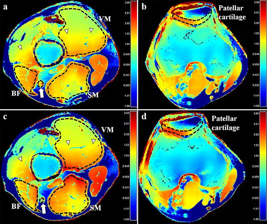
www.nature.com/scientificreports/
MD Mean diffusivity
ICC Intraclass correlation coefficient
Electrical conductivity is an intrinsic property of a material that represents the capability to transfer electrical
current inside the m edium1. In biological tissues, it is closely related to water content, intracellular and extracel-
lular fluid volumes, ion concentration, and the cellular membrane permeability, thus has been considered to be
a fundamental biophysical p roperty2,3. As several experimental studies have shown that conductivity can reflect
pathologic status as well as tissue t ype4–7, it has emerged as a potentially important tissue biomarker for clinical
diagnostics8,9.
While previous investigations mostly relied on ex vivo m easurements4–7, the first non-invasive in vivo assess-
ment of conductivity was made using the electrical impedance tomography (EIT)10. Among multiple efforts to
improve non-invasive conductivity imaging, MR-EIT provided higher spatial resolution and eliminated the need
to solve the ill-posed inverse problem in EIT11. However, as it required injection of electrical current into the
body, safety concerns were r aised9. Another technique called magnetic induction tomography did not involve
direct contact with the subject, nevertheless, this non-MRI-based method exhibited poor spatial resolution12.
Based on the concept of deriving conductivity from the measured MR s ignals13, another non-invasive
approach termed “MR-electrical properties tomography (MR-EPT)” has been introduced by Katscher et al.14.
They reconstructed tissue conductivity from the measured B1+ field generated by the radiofrequency (RF) coil. It
is considered to be advantageous regarding practicability, as it can be acquired using standard MRI system with
a regular coil and does not apply externally mounted electrodes or c urrent8. With increasing interest, there has
been continuous progress in the research of MR-EPT to validate it15, prove its feasibility16, and estimate specific
absorption rate (SAR)17. Whilst several clinical studies have investigated MR-EPT in various organs including
breast18,19, brain20, and liver21, the number of studies that utilized MR-EPT in musculoskeletal tissues has been
limited22.
Thus, the purpose of this study was to investigate whether in vivo imaging is feasible in musculoskeletal tis-
sues using MR-EPT by evaluating the conductivity of muscle, cartilage, and peripheral nerves around the knee
joint. Under the hypothesis that conductivity could reflect physiologic changes, this study also sought to explore
whether the conductivity of musculoskeletal tissues changes after exercise, and to interpret their changes with
reference to other quantitative measurements including T2, T2* relaxation times (RT) and diffusion tensor
imaging (DTI) parameters.
Materials and methods
This prospective study was approved by the institutional review board (Samsung Medical Center, IRB File No.
2019-11-032) and registered at cris.nih.go.kr (KCT0004839). After being advised of the purpose of the study, all
subjects gave written informed consent. The study was conducted in accordance with the declaration of Helsinki.
Study population. According to a previous study22, the mean and standard deviation of muscle conductiv-
ity using MR-EPT has been reported to be 0.93 S/m (Siemens per meter = Ω−1 m−1) and 0.26 S/m, respectively.
The sample size (n) needed to construct a 95% confidence interval with a margin of error of 0.17 S/m was pro-
spectively calculated using the following equation: n = 1.962 × SD2/d2, where SD and d are the standard deviation
of muscle conductivity and the margin of error, respectively. Therefore, the sample size was calculated to be nine.
Assuming dropout rate to be 10%, ten subjects were required.
Ten healthy adults were recruited who had body mass index between 18.5 and 25.0, without any discomfort
in their lower extremities, previous history of internal derangement, surgery in the right knee, or contraindica-
tion to MRI such as claustrophobia.
Magnetic resonance imaging acquisition. All volunteers underwent baseline imaging using a 3.0-T
MRI scanner (Ingenia CX, Philips Medical Systems) and a 16-channel knee coil. For conductivity assessment, a
three-dimensional (3D) balanced steady-state free precession (bSSFP) (balanced fast field echo [bFFE], Philips
Medical Systems) sequence was chosen; this sequence was selected due to its relatively benign off-resonance
behavior and robustness against unwanted phase contribution from flow, motion, and eddy current8. Both mag-
nitude and phase images were obtained in the axial plane. To evaluate the test–retest reliability of conductivity,
all volunteers underwent two iterations of the bSSFP sequence. Thereafter, T2 map (T2-weighted multi-echo
spin-echo sequence), T2* map (T2*-weighted multi-echo fast-field echo sequence with ∆B0 correction), and DTI
(single-shot echo-planar imaging) in the axial planes were acquired. T2 and T2* maps were computed using a
pixel-by-pixel basis, mono-exponential, non-negative least-square fitting algorithm. For DTI, diffusion gradi-
ents were applied in six directions and diffusion encoding was done with monopolar gradient pulses. Detailed
MRI parameters are summarized in Table 1.
Exercise protocol and post‑exercise imaging. To test the effect of loading, the volunteers performed
squatting exercise outside the MRI scanner after baseline imaging as described in a previous literature23. Stand-
ing with weight equally distributed and the feet separated shoulder width apart, they were asked to stand in a
position of knee flexion at 90° bilaterally. Keeping the knees not moving past the toes, they held this position
for 3 s, followed by repositioning to stand upright. They performed 60 repetitions under supervision by an
observer to ensure identical exercise among the volunteers. After exercising, the volunteers were immediately
repositioned on the MR table for post-exercise imaging using the same sequences and protocols as the baseline
imaging, including two iterations of the bSSFP sequence. The first and second post-exercise bSSFP sequences
were acquired 2 and 6 min after exercise cessation in all volunteers, respectively. Volunteers’ skin was marked
Scientific Reports | (2022) 12:73 | https://doi.org/10.1038/s41598-021-03928-y 2
Vol:.(1234567890)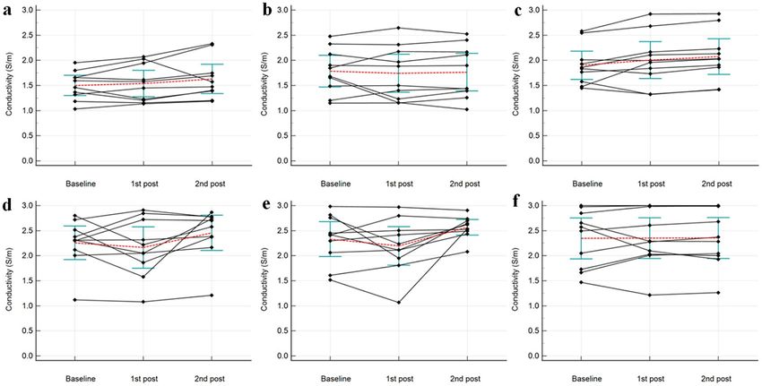
www.nature.com/scientificreports/
bSSFP T2 map T2* map DTI
TR (ms) 4.5302 1735.2 61.8963 3399.1
TE (ms) 2.265 13 (13, 6)* 2.83 (2.354, 15)* 61.344
Acquisition matrix 224 × 222 400 × 286 400 × 400 116 × 114
Reconstruction matrix 352 × 352 400 × 400 448 × 448 128 × 128
Pixel spacing (mm) 0.568 0.500 0.446 1.562
Field of view (cm) 20 20 20 20
Slice Thickness/gap (mm) 1/0 3/0.3 3/0.3 3/0
b values – – – 0, 600
Number of averages 2 1 1 2
Number of slices 80 20 20 30
Echo train length 1 6 15 57
Parallel reduction factor 1 2 2.1 2
Flip angle (°) 30 90 25 90
Acquisition time 4 min 12 s 4 min 9 s 3 min 14 s 3 min 34 s
Table 1. Parameters of MR sequences. TR, repetition time; TE, echo time; bSSFP, balanced steady-state free
precession; DTI, diffusion tensor imaging. *Data are the first TE with ΔTE and the number of TE values in
parentheses.
under the guidance of integrated laser to maintain identical imaging position between the baseline and post-
exercise imaging.
EPT reconstruction. After data acquisition, all images were transferred to an independent workstation for
analysis with manufacturer-supplied software (Extended Philips Research Software Solution [EXPRESS], Philips
Healthcare). The conductivity maps were reconstructed from the phase images of the 3D bSSFP sequence. To
convert the phase information to conductivity (σ), the following equation (assuming constant B1 magnitude)
was used:
σ = ��+ /(µω)
where ω = Larmor frequency, Δ = Laplacian operator, μ = magnetic permeability of tissue (assumed to be equal to
magnetic permeability of free space), and Φ+ = RF transmit phase estimated as half of the measured transceive
phase Φ± (i.e., Φ+ ≈ Φ±/2)8. Care has to be taken that Φ± does not show any phase wraps when applying this divi-
sion by two. However, since the total phase span across the field of view has been roughly 60° for the experiments
in this study, no dedicated phase unwrapping was needed. The second derivative required for Δ was performed
numerically by fitting a local parabola to a number N of voxels (“kernel”) on each side of the respective target
voxel of Φ±. A maximum number of N was chosen as Nmax = 10 and reduced as soon as the bSSFP magnitude
of a kernel voxel deviates more than 10% from the target voxel, providing a suitable trade-off between too low
signal-to-noise ratio (for too small N) and decreased image resolution (for too large N) and avoids the typical
boundary artifacts of EPT. As the Laplacian operator inevitably leads to noise amplification, a bilateral median
filter was applied to the conductivity resulting from those equations, again applying the locally shaped kernel as
done for the differentiation step. This approach has successfully been applied in previous studies for brain tumor
conductivity20,24 and similarly also for breast tumor c onductivity19,25.
Image analysis. Two board-certified radiologists (readers I and II; 5 and 1 years of experience in musculo-
skeletal imaging, respectively) analyzed the MRIs. Among T2-weighted images with six different echo times, one
was selected and regarded as anatomical reference that best differentiated subchondral bone, articular cartilage,
and joint fluid from the cartilage. Using the manufacturer-supplied software (Extended Philips Research Soft-
ware Solution [EXPRESS], Philips), conductivities of muscles, cartilages, and nerves were measured by placing
regions of interests (ROIs) on the magnitude image of the 3D bSSFP sequence using freehand drawing tools
according to the following criteria (Fig. 1):
(1) Muscles: At the level of the distal thigh, the vastus medialis (VM), semimembranosus muscles (SM), and
biceps femoris muscle, including both long and short heads (BF) were selected because they had sufficient
cross-sectional area. The ROIs were placed on each muscle so that the boundaries were within 1–2 mm
from the muscle fascia.
(2) Cartilages: Axial planes that revealed the maximum thickness of the patellar and trochlear cartilages were
selected for evaluation. The ROIs were placed to cover the entire cartilage, encompassing both deep and
superficial cartilage, and medial and lateral facets; joint fluid or subchondral bone were carefully avoided.
(3) Nerve: At the same axial plane as that for muscle analysis, the ROIs were carefully drawn to fall within the
visualized boundary of the tibial nerve, excluding the perineural vessels.
Scientific Reports | (2022) 12:73 | https://doi.org/10.1038/s41598-021-03928-y 3
Vol.:(0123456789)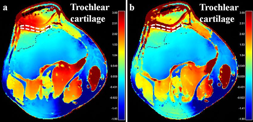
www.nature.com/scientificreports/
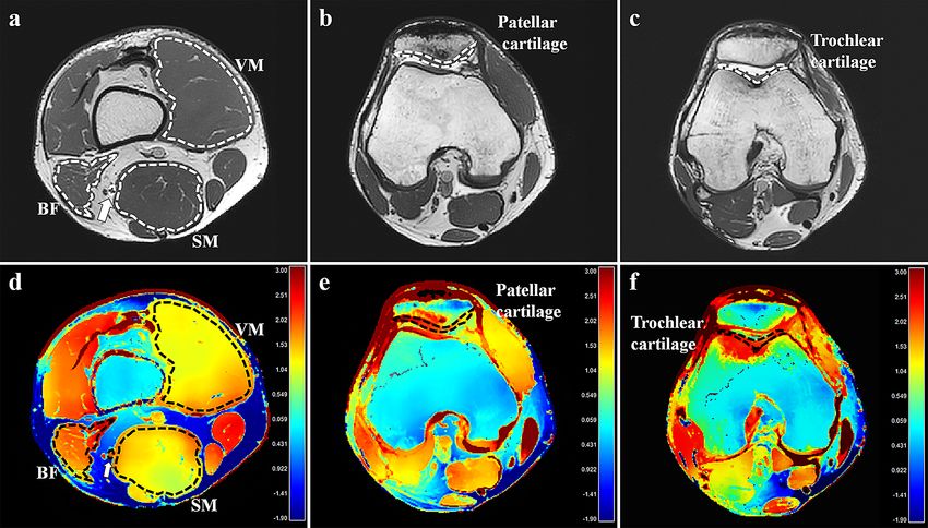
Figure 1. An example of conductivity analysis in the right knee of a 30-year old male volunteer. Regions of
interest (ROIs) were placed in the vastus medialis (VM), semimembranosus (SM) muscles, biceps femoris
muscle, including both long and short heads (BF), tibial nerve at the distal thigh level, and patellar and trochlear
cartilage on the axial three-dimensional balanced fast-field echo sequence (a–c). ROIs with identical shapes,
sizes, and positions were automatically generated on the conductivity map (d–f). The unit for the scale bars
is S/m. Arrows, tibial nerve; dotted lines, ROIs.
Dedicated software (IntelliSpace Portal, version 10.0; Philips) was used for image processing and ROI place-
ment on the T2, T2* maps, and DTI using the same criteria and anatomical reference images. The mean T2 and
T2* RTs, fractional anisotropy (FA), and mean diffusivity (MD) of the same muscles, cartilages, and nerves were
measured at the corresponding areas.
Statistical analysis. Paired t-test was used to explore if the post-exercise values varied from the baseline
imaging. Test–retest reliability between conductivities obtained from the 1st and 2nd baseline bSSFP sequences
by reader I and interobserver agreement between the two readers were assessed using the intraclass correlation
coefficient (ICC). An ICC of 1.0 was considered to represent perfect agreement; 0.81–0.99, almost perfect agree-
ment; 0.61–0.80, substantial agreement; 0.41–0.60, moderate agreement; 0.21–0.40, fair agreement; and 0.20 or
less, slight a greement26. All statistical analyses were performed using MedCalc version 19.0.7 (MedCalc Software
Ltd). p values less than 0.05 were considered to indicate statistical significance.
Results
The subjects constituted of five men and five women volunteers, ranging in age from 24 to 30 years
(26.8 ± 1.8 years). The patellar and trochlear cartilages in two volunteers, were excluded on second baseline imag-
ing due to severe artifacts. The duration of exercise ranged from 3 min 56 s to 7 min 51 s (6 min 11 s ± 1 min 17 s).
Interobserver agreement and test–retest reliability. Because there was almost perfect interobserver
agreement on measurements of conductivity in muscles, cartilages, and nerves, data obtained by one of the read-
ers were used. The result of the test–retest reliability of the baseline conductivity was almost perfect in all muscles
and the tibial nerve. Cartilages tended to show lower test–retest reliability, which were regarded as substantial
(Table 2).
Baseline conductivity measurements. The range of baseline conductivity was as follows: all muscles,
1.03–2.58 S/m; VM muscle, 1.03–1.95 S/m; SM muscle, 1.15–2.48 S/m; BF muscle, 1.45–2.58 S/m; all cartilages,
1.12–2.98 S/m; patellar cartilage, 1.11–2.80 S/m; trochlear cartilage, 1.51–2.98 S/m; tibial nerve, 1.47–3.00 S/m.
Post‑exercise changes of conductivity. Means and standard deviations of conductivity in muscles,
cartilages, and nerves during the baseline, first, and second post-exercise imaging are summarized in Table 3.
Conductivity of all muscles, the BF muscle, and all cartilages on the second post-exercise imaging significantly
Scientific Reports | (2022) 12:73 | https://doi.org/10.1038/s41598-021-03928-y 4
Vol:.(1234567890)www.nature.com/scientificreports/
Test–retest reliability Interobserver agreement
All muscles 0.89 (0.79–0.95) 0.98 (0.97–0.98)
VM muscle 0.80 (0.41–0.95) 0.96 (0.93–0.98)
SM muscle 0.96 (0.84–0.99) 0.97 (0.95–0.98)
BF muscle 0.84 (0.51–0.96) 0.99 (0.97–0.99)
All cartilages 0.67 (0.28–0.87) 0.99 (0.98–0.99)
Patellar cartilage 0.71 (0.09–0.94) 0.98 (0.97–0.99)
Trochlear cartilage 0.64 (− 0.05–0.91) 0.99 (0.97–0.99)
Tibial nerve 0.89 (0.63–0.97) 0.92 (0.85–0.96)
Table 2. Test–retest reliability and interobserver agreement for conductivity measurement. Data are intraclass
correlation coefficients and 95% confidence intervals in the parentheses. CI, confidence interval; VM, vastus
medialis; SM, semimembranosus; BF, biceps femoris; and ICC, intraclass correlation coefficient.
95% CI of 95% CI of
Baseline 1st Post-exercise differences* p value* 2nd Post-exercise differences† p value†
All muscles 1.73 ± 0.40 1.76 ± 0.50 − 0.05 to + 0.12 0.428 1.82 ± 0.50 + 0.00 to + 0.19 0.048
VM muscle 1.50 ± 0.28 1.54 ± 0.37 − 0.08 to + 0.16 0.482 1.63 ± 0.41 − 0.04 to + 0.30 0.126
SM muscle 1.79 ± 0.44 1.74 ± 0.53 − 0.23 to + 0.15 0.626 1.76 ± 0.52 − 0.21 to + 0.17 0.819
BF muscle 1.90 ± 0.39 2.00 ± 0.51 − 0.06 to + 0.27 0.191 2.08 ± 0.50 + 0.02 to + 0.32 0.029
All cartilages 2.29 ± 0.47 2.18 ± 0.54 − 0.29 to + 0.07 0.202 2.51 ± 0.37 + 0.07 to + 0.36 0.006
Patellar cartilage 2.26 ± 0.47 2.16 ± 0.58 − 0.38 to + 0.20 0.483 2.46 ± 0.49 − 0.01 to + 0.41 0.061
Trochlear cartilage 2.33 ± 0.49 2.20 ± 0.54 − 0.41 to + 0.14 0.299 2.57 ± 0.22 − 0.01 to + 0.48 0.060
Tibial nerve 2.35 ± 0.57 2.35 ± 0.57 − 0.20 to + 0.21 0.953 2.36 ± 0.57 − 0.22 to + 0.24 0.927
Table 3. Conductivity before and after exercise. Data are mean ± standard deviation (S/m). VM, vastus
medialis; SM, semimembranosus; BF, biceps femoris; and CI, confidence interval. *Between the baseline and
1st post-exercise MRI. † Between the baseline and 2nd post-exercise MRI.
changed by + 5.41 ± 14.36% (p = 0.048), + 9.05 ± 11.07% (p = 0.029), and + 9.49 ± 13.69% (p = 0.006), respec-
tively [mean ± standard deviation], with an overall increase from the baseline; conductivity of the VM mus-
cle, patellar, and trochlear cartilages tended to increase on the second post-exercise imaging, which changed
by + 8.59 ± 16.12% (p = 0.126), + 8.84 ± 4.13% (p = 0.061), and + 10.12 ± 4.71% (p = 0.060), respectively (Figs. 2, 3,
4). All conductivities of the first post-exercise imaging and conductivity of the tibial nerve on the second post-
exercise imaging were not significantly different from the baseline imaging.
Post‑exercise changes of other quantitative parameters. After exercise, the T2 RT, T2* RT, FA,
and MD of the VM muscle changed by + 17.54 ± 11.10% (p < 0.001), + 19.89 ± 8.37% (p < 0.001), + 5.98 ± 6.11%
(p = 0.013), and + 14.89 ± 4.42% (p < 0.001), respectively, with an overall increase compared to the baseline. In
contrast, the BF muscle showed overall post-exercise decrease of the T2 RT, T2* RT, and MD, which changed by
− 3.82 ± 4.39% (p = 0.022), − 3.79 ± 4.66% (p = 0.030), and − 3.59 ± 2.93% (p = 0.004) from the baseline, respec-
tively. Regarding all muscles, overall post-exercise increase was observed in the T2* RT and FA, which changed
by + 4.34 ± 11.97% (p = 0.018) and + 3.52 ± 6.72% (p = 0.012) from the baseline, respectively. No other significant
differences in the T2 RT, T2* RT, FA, and MD were noted between the baseline and post-exercise imaging
(Table 4).
Discussion
This study measured in vivo conductivity of muscles, cartilages, and nerves around the knee joint in normal
volunteers using MR-EPT and showed its feasibility. Additionally, this study revealed that post-exercise conduc-
tivity significantly changed with a tendency to increase in muscles and cartilages at 6 min after exercise cessation.
In previous animal studies, results of muscle conductivity assessment observed a large variation ranging
between 0.56 and 1.05 S/m27–29, probably due to various species and study conditions. In human subjects, muscle
conductivity has been reported to be 0.62 S/m30 and 0.93 S/m22. In ex vivo studies, conductivity of cartilages
and nerves were reported to be 0.51–1.14 S/m29,31 and 0.39 S/m29, respectively. Though different experimental
conditions make direct comparison difficult, the conductivity values of our study were higher than those of
previous investigations.
Compared to the conductivity maps in previous studies on MR-EPT18,20, maps in this study were suspected to
suffer from B1 inhomogeneity. The bSSFP sequence is known to have relative robustness against B0 inhomogene-
ity, as long as banding artifacts from signal voids are avoided, and in fact B0 inhomogeneities are too small to
produce those banding artifacts in the knee images of this study; yet, conductivity reconstruction is vulnerable
to B1 inhomogeneity8. Conductivity reconstruction as applied in this study is based on B1 phase only, i.e., based
Scientific Reports | (2022) 12:73 | https://doi.org/10.1038/s41598-021-03928-y 5
Vol.:(0123456789)www.nature.com/scientificreports/
Figure 2. Baseline (a, b) and the post-exercise conductivity map (c, d) in a 28-year old male volunteer.
Compared to the baseline, conductivity of the vastus medialis muscles and patellar cartilage increased from
1.033 to 1.188 S/m, and from 1.119 to 1.450 S/m, respectively. B1 inhomogeneity is noted across field of view,
shown as demarcated areas with increased conductivity in red-colored zones (arrowheads). The unit for the
scale bars is S/m. BF, biceps femoris muscle; SM, semimembranosus muscle; VM, vastus medialis muscle;
arrows, tibial nerve; dotted lines, ROIs.
Figure 3. Baseline (a) and the post-exercise conductivity map (b) in a 28-year old male volunteer. Compared to
the baseline, conductivity of the trochlear cartilage increased from 1.887 to 2.539 S/m. The unit for the scale bars
is S/m. dotted lines, ROIs.
on the assumption of a constant B1 magnitude. It has been reported that a violation of this assumption leads
to an artificial increase of reconstructed conductivity, contributing to the observed high conductivity v alues32.
A phantom simulation as described in the Supplementary material underlines this effect, leading to roughly
twice the expected conductivity as a consequence of the EPT assumptions applied. A future study shall include
the additional measurement of B1 magnitude to exclude this artificial conductivity increase. Nevertheless, as B1
inhomogeneity is similar for all scans in this study, it can be expected that the observed exercise-induced increase
of conductivity is not affected by this issue. Furthermore, this study adopted the so-called “transceive phase
assumption”, estimating the absolute B1+ phase Φ+ to be half of the transceive phase Φ± as the B1+ phase is not
directly measurable by standard MR s equences15,32,33. Even though it has been widely used, violation against this
assumption is thought to lower the accuracy of conductivity evaluation. Phase error has been reported to be larger
Scientific Reports | (2022) 12:73 | https://doi.org/10.1038/s41598-021-03928-y 6
Vol:.(1234567890)www.nature.com/scientificreports/
Figure 4. Graphs showing change of conductivity of vastus medialis muscle (a), semimembranosus muscle (b),
biceps femoris muscle (c), patellar cartilage (d), trochlear cartilage (e), and tibial nerve (f) for each volunteer.
The mean values are represented by red dotted lines, 95% confidence intervals of mean values by blue green
bars, respectively.
at the peripheral regions indicating that the merit of this assumption d eteriorates16,34. In addition, geometric
asymmetry may lead to unequal contributions of the transmission and reception process in the total transceive
phase33. It can also be prone to inaccuracies when imaging subjects with asymmetrical electrical p roperties35. In
this context, substantial phase error might have been produced in this study. As extremities are hardly scanned
in the isocenter area and are inherently asymmetric with right- or left-sided predilection, this phase error could
be regarded as one of the major problems to be resolved for implementing MR-EPT in musculoskeletal imaging.
Given that the previous s tudy22 from which we estimated the sample size examined pelvic region, wide range of
conductivity with relatively large SD in our study also might be explained by aforementioned reasons. Despite
of previous study that validated MR-EPT15, our study suggests that it may be vulnerable to reconstruction error
in musculoskeletal regions requiring further validation.
The post-exercise T2 and T2* RTs, FA, and MD significantly increased in the VM muscle, which was compara-
ble to the findings of previous s tudies36,37. Osmotic shift, water accumulation, increase in volume of intracellular
space of perfused muscle and intracellular acidification increases T2 RT36–40, whereas blood inflow exceeding
oxygen extraction fraction increases T2* R T36,41. For DTI parameters, tightening of muscle fibers and changes
in intra- and extracellular volume, pseudodiffusion due to increased blood volume are suggested to increase FA
and MD, r espectively40,42. In contrast, the post-exercise T2, T2* RT, and MD of the BF muscle decreased in this
study, contrary to the VM muscle. As squatting elicits greater activity of quadriceps relative to other m uscles43,
decreased T2, T2* RT, and MD may imply compensatory vasoconstriction in the BF muscle.
On the other hand, conductivity tended to increase in both VM and BF muscles and cartilages on the second
post-exercise MRI compared to the baseline. While conductivity is affected by both water content and tissue
sodium concentration44, increased conductivity could not be explained by increased water content as T2 RT
were decreased in the BF muscle and not changed in the cartilages. Thus, it could be reasonable to presume
that increased conductivity may reflect increased tissue sodium concentration, which probably occurs several
minutes after the exercise cessation rather than immediate post-exercise period. However, considering that the
duration of exercise varied between the volunteers and that there was a difference in the pattern of change in
conductivity after exercise as shown in Fig. 4, additional research is required to prove the timing of change in
conductivity after exercise. In this context, exercise-induced time course changes of conductivity using a rapid
sequential acquisition of MR-EPT would be another interesting topic of future investigation.
Our result showing changes of conductivity in muscle is partially comparable to those of previous studies
reporting signal intensity increase of muscle after exercise using sodium MRI45,46. Whereas sodium MRI is still
challenging due to limitations in hardware and software, MR-EPT is advantageous as it uses standard MR scan-
ners. Considering usefulness of sodium MRI in evaluating early cartilage d egeneration47, it could be reasonable
to consider cartilage imaging as one of the promising applications of MR-EPT in the musculoskeletal regions.
However, conductivity of the SM muscle did not show tendency of post-exercise increase. Although we presumed
that no significant physiologic change occurred in the SM muscle after exercise considering all the other param-
eters were also not changed, the basis of this result remains unclear. Furthermore, the fact that the differences
between baseline and post-exercise conductivity in muscles and cartilages were significant only when they were
Scientific Reports | (2022) 12:73 | https://doi.org/10.1038/s41598-021-03928-y 7
Vol.:(0123456789)www.nature.com/scientificreports/
Baseline Post-exercise 95% CI of difference* p value*
T2 RT (ms)
All muscles 38.39 ± 3.17 39.91 ± 4.29 − 0.16 to + 3.20 0.074
VM muscle 37.35 ± 1.71 43.90 ± 4.03 + 3.58 to + 9.52 < 0.001
SM muscle 35.89 ± 1.01 35.50 ± 1.04 − 1.24 to + 0.46 0.329
BF muscle 41.93 ± 2.52 40.33 ± 1.57 − 2.92 to − 0.28 0.022
All cartilages 42.80 ± 7.71 42.06 ± 6.98 − 1.81 to + 0.34 0.168
Patellar cartilage 37.49 ± 6.04 37.27 ± 5.58 − 1.17 to + 0.73 0.612
Trochlear cartilage 48.10 ± 5.14 46.85 ± 4.56 − 3.36 to + 0.86 0.214
Tibial nerve 54.82 ± 5.57 53.93 ± 4.75 − 2.38 to + 0.60 0.208
T2* RT (ms)
All muscles 26.13 ± 1.36 27.61 ± 3.66 + 0.28 to + 2.70 0.018
VM muscle 26.80 ± 0.92 32.13 ± 2.11 + 3.73 to + 6.93 < 0.001
SM muscle 25.75 ± 1.24 25.86 ± 1.27 − 0.92 to + 1.14 0.815
BF muscle 25.83 ± 1.67 24.85 ± 1.55 − 1.84 to − 0.12 0.030
All cartilages 31.56 ± 6.36 31.27 ± 6.15 − 1.26 to + 0.68 0.538
Patellar cartilage 27.05 ± 4.89 26.80 ± 4.82 − 1.45 to + 0.95 0.648
Trochlear cartilage 36.07 ± 4.03 35.74 ± 3.50 − 2.12 to + 1.46 0.686
Tibial nerve 25.56 ± 4.67 25.17 ± 5.51 − 2.02 to + 1.24 0.601
FA
All muscles 0.247 ± 0.035 0.255 ± 0.034 + 0.002 to + 0.014 0.012
VM muscle 0.234 ± 0.016 0.248 ± 0.017 + 0.004 to + 0.024 0.013
SM muscle 0.219 ± 0.017 0.227 ± 0.023 − 0.002 to + 0.018 0.104
BF muscle 0.287 ± 0.021 0.289 ± 0.027 − 0.012 to + 0.016 0.751
All cartilages 0.134 ± 0.042 0.124 ± 0.030 − 0.028 to + 0.009 0.298
Patellar cartilage 0.129 ± 0.038 0.113 ± 0.017 − 0.039 to + 0.007 0.149
Trochlear cartilage 0.138 ± 0.047 0.135 ± 0.036 − 0.037 to + 0.031 0.844
Tibial nerve 0.539 ± 0.011 0.552 ± 0.048 − 0.054 to + 0.080 0.672
MD (× 10–3 mm2/s)
All muscles 1.57 ± 0.08 1.59 ± 0.26 − 0.06 to + 0.11 0.570
VM muscle 1.63 ± 0.06 1.87 ± 0.05 + 0.19 to + 0.29 < 0.001
SM muscle 1.52 ± 0.06 1.41 ± 0.27 − 0.33 to + 0.10 0.269
BF muscle 1.56 ± 0.10 1.51 ± 0.08 − 0.09 to − 0.02 0.004
All cartilages 1.68 ± 0.14 1.66 ± 0.23 − 0.15 to + 0.09 0.645
Patellar cartilage 1.69 ± 0.14 1.62 ± 0.30 − 0.30 to + 0.16 0.530
Trochlear cartilage 1.68 ± 0.14 1.70 ± 0.12 − 0.10 to + 0.13 0.792
Tibial nerve 1.15 ± 0.16 1.08 ± 0.16 − 0.19 to + 0.05 0.246
Table 4. Quantitative measurements before and after exercise. Data are mean ± standard deviation. VM, vastus
medialis; SM, semimembranosus; BF, biceps femoris; RT, relaxation time; FA, fractional anisotropy; MD, mean
diffusivity; and CI, confidence interval. *Between the baseline and post-exercise MRI.
grouped except for the BF muscle requires future investigation to elucidate its true significance. In addition to
the technical issues regarding B1 inhomogeneity, relatively low test–retest reliability in the cartilage possibly due
to their small size and curved shape is another hurdle that should be overcome.
This study had several limitations. First, the MR-EPT technique was not validated in the musculoskeletal
regions. Validation using a knee-sized phantom and conductivity probe could help proving its reliability in
musculoskeletal imaging. Second, substantial inhomogeneity was noted in the conductivity maps with regions
of increased conductivity, as described above. Further optimization would be mandatory, which may provide
conductivity values closer to the values reported in previous investigations. Third, the time intervals between
exercise cessation and acquisition of each sequence for quantitative measurements were variable. The duration of
exercise was also variable among the volunteers, which also may have influenced the study results particularly in
post-exercise changes of conductivity. Fourth, misalignment of knee joints between the baseline and post-exercise
scans could have been possible. Intelligent software which automatically plans the scanning geometries would
be helpful, in addition to our effort using skin marking and integrated laser. Finally, temperature measurements
of target tissues were not performed, assuming them to be 37 °C for both baseline and post-exercise MRI. As
temperature coefficient of conductivity variation is about 2%/°C48, change of temperature after exercise may
have affected our study results.
Scientific Reports | (2022) 12:73 | https://doi.org/10.1038/s41598-021-03928-y 8
Vol:.(1234567890)www.nature.com/scientificreports/
In conclusion, in vivo conductivity measurement was feasible in musculoskeletal tissues using MR-EPT
around the knee joint. Although technological hurdles should be overcome that might result in artificial increase
of conductivity values and relatively poor reproducibility of cartilage conductivity, significant post-exercise
change in conductivity may suggest its potential as a biomarker to reflect physiologic status of musculoskeletal
tissues. Further clinical studies with validation based on this initial experience of MR-EPT would be mandatory
to elucidate true significance of conductivity in musculoskeletal imaging and to expand its applications particu-
larly to indirect assessment of tissue sodium concentration.
Received: 4 February 2021; Accepted: 10 December 2021
References
1. Kandadai, M. A., Raymond, J. L. & Shaw, G. J. Comparison of electrical conductivities of various brain phantom gels: Developing
a ‘brain gel model’. Mater. Sci. Eng. C-Mater. 32, 2664–2667. https://doi.org/10.1016/j.msec.2012.07.024 (2012).
2. Gabriel, S., Lau, R. W. & Gabriel, C. The dielectric properties of biological tissues: II. Measurements in the frequency range 10 Hz
to 20 GHz. Phys. Med. Biol. 41, 2251–2269, https://doi.org/10.1088/0031-9155/41/11/002 (1996).
3. Hurt, W. D. Multiterm Debye dispersion relations for permittivity of muscle. IEEE Trans. Biomed. Eng. 32, 60–64. https://doi.org/
10.1109/TBME.1985.325629 (1985).
4. Surowiec, A. J., Stuchly, S. S., Barr, J. B. & Swarup, A. Dielectric properties of breast carcinoma and the surrounding tissues. IEEE
Trans. Biomed. Eng. 35, 257–263. https://doi.org/10.1109/10.1374 (1988).
5. Jossinet, J. The impedivity of freshly excised human breast tissue. Physiol. Meas. 19, 61–75. https://doi.org/10.1088/0967-3334/
19/1/006 (1998).
6. Fallert, M. A. et al. Myocardial electrical impedance mapping of ischemic sheep hearts and healing aneurysms. Circulation 87,
199–207. https://doi.org/10.1161/01.cir.87.1.199 (1993).
7. Haemmerich, D. et al. In vivo electrical conductivity of hepatic tumours. Physiol. Meas. 24, 251–260. https://doi.org/10.1088/
0967-3334/24/2/302 (2003).
8. Katscher, U., Kim, D. H. & Seo, J. K. Recent progress and future challenges in MR electric properties tomography. Comput. Math.
Methods Med. 2013, 546562. https://doi.org/10.1155/2013/546562 (2013).
9. Zhang, X., Liu, J. & He, B. Magnetic-resonance-based electrical properties tomography: a review. IEEE Rev. Biomed. Eng. 7, 87–96.
https://doi.org/10.1109/RBME.2013.2297206 (2014).
10. Holder, D. S. Electrical Impedance Tomography: Methods, History and Applications (Institute of Physics Publishing, 2005).
11. Seo, J. K., Yoon, J. R., Woo, E. J. & Kwon, O. Reconstruction of conductivity and current density images using only one component
of magnetic field measurements. IEEE Trans. Biomed. Eng. 50, 1121–1124. https://doi.org/10.1109/Tbme.2003.816080 (2003).
12. Korzhenevskii, A. V. & Cherepenin, V. A. Magnetic induction tomography. Radiotekh. Elektron. (Moscow) 42, 506–512 (1997).
13. Haacke, E., Petropoulos, L., Nilges, E. & Wu, D. Extraction of conductivity and permittivity using magnetic resonance imaging.
Phys. Med. Biol. 36, 723 (1991).
14. Katscher, U., Hanft, M., Vernickel, P. & Findeklee, C. Electric properties tomography (EPT) via MRI. Proc. Intl. Soc. Mag. Reson.
Med. 14 (2006).
15. Katscher, U. et al. Determination of electric conductivity and local SAR via B1 mapping. IEEE Trans. Med. Imaging 28, 1365–1374.
https://doi.org/10.1109/TMI.2009.2015757 (2009).
16. Balidemaj, E. et al. Feasibility of electric property tomography of pelvic tumors at 3T. Magn. Reson. Med. 73, 1505–1513. https://
doi.org/10.1002/mrm.25276 (2015).
17. Voigt, T., Homann, H., Katscher, U. & Doessel, O. Patient-individual local SAR determination: In vivo measurements and numeri-
cal validation. Magn. Reson. Med. 68, 1117–1126. https://doi.org/10.1002/mrm.23322 (2012).
18. Mori, N. et al. Diagnostic value of electric properties tomography (EPT) for differentiating benign from malignant breast lesions:
Comparison with standard dynamic contrast-enhanced MRI. Eur. Radiol. 29, 1778–1786. https://doi.org/10.1007/s00330-018-
5708-4 (2019).
19. Kim, S. Y. et al. Correlation between conductivity and prognostic factors in invasive breast cancer using magnetic resonance electric
properties tomography (MREPT). Eur. Radiol. 26, 2317–2326. https://doi.org/10.1007/s00330-015-4067-7 (2016).
20. Tha, K. K. et al. Noninvasive electrical conductivity measurement by MRI: A test of its validity and the electrical conductivity
characteristics of glioma. Eur. Radiol. 28, 348–355. https://doi.org/10.1007/s00330-017-4942-5 (2018).
21. Stehning, C., Voigt, T., Karkowski, P. & Katscher, U. Electric properties tomography (EPT) of the liver in a single breathhold using
SSFP. Proc. Intl. Soc. Mag. Reson. Med. 20, abstract 386 (2012).
22. Balidemaj, E. et al. In vivo electric conductivity of cervical cancer patients based on B(1)(+) maps at 3T MRI. Phys. Med. Biol. 61,
1596–1607. https://doi.org/10.1088/0031-9155/61/4/1596 (2016).
23. Liess, C., Lusse, S., Karger, N., Heller, M. & Gluer, C. C. Detection of changes in cartilage water content using MRI T2-mapping
in vivo. Osteoarthr. Cartil. 10, 907–913. https://doi.org/10.1053/joca.2002.0847 (2002).
24. Park, J. E. et al. Low conductivity on electrical properties tomography demonstrates unique tumor habitats indicating progression
in glioblastoma. Eur. Radiol. 31, 6655–6665. https://doi.org/10.1007/s00330-021-07976-w (2021).
25. Suh, J. et al. Noncontrast-enhanced MR-based conductivity imaging for breast cancer detection and lesion differentiation. J. Magn.
Reson. Imaging 54, 631–645. https://doi.org/10.1002/jmri.27655 (2021).
26. Landis, J. R. & Koch, G. G. The measurement of observer agreement for categorical data. Biometrics 33, 159–174 (1977).
27. Oswald, K. Messung der leitfahigkeit und Dielektrizitatkonstante biologischer Gewebe un Flussigkeiten bei kurzen Wellen. Hochfreq
Tech Elektroakust 49, 40–49 (1937).
28. Stoy, R. D., Foster, K. R. & Schwan, H. P. Dielectric properties of mammalian tissues from 0.1 to 100 MHz: A summary of recent
data. Phys. Med. Biol. 27, 501–513. https://doi.org/10.1088/0031-9155/27/4/002 (1982).
29. Gabriel, C. & Gabriel, S. Compilation of the Dielectric Properties of Body Tissues at RF and Microwave Frequencies (Dept of Physics,
King’s Coll, 1996).
30. Joines, W. T., Zhang, Y., Li, C. & Jirtle, R. L. The measured electrical properties of normal and malignant human tissues from 50
to 900 MHz. Med. Phys. 21, 547–550. https://doi.org/10.1118/1.597312 (1994).
31. Binette, J. S., Garon, M., Savard, P., McKee, M. D. & Buschmann, M. D. Tetrapolar measurement of electrical conductivity and
thickness of articular cartilage. J. Biomech. Eng. 126, 475–484. https://doi.org/10.1115/1.1785805 (2004).
32. Voigt, T., Katscher, U. & Doessel, O. Quantitative conductivity and permittivity imaging of the human brain using electric proper-
ties tomography. Magn. Reson. Med. 66, 456–466. https://doi.org/10.1002/mrm.22832 (2011).
33. van Lier, A. L. et al. B1(+) phase mapping at 7 T and its application for in vivo electrical conductivity mapping. Magn. Reson. Med.
67, 552–561. https://doi.org/10.1002/mrm.22995 (2012).
34. van Lier, A. L. et al. Electrical properties tomography in the human brain at 1.5, 3, and 7T: A comparison study. Magn. Reson. Med.
71, 354–363. https://doi.org/10.1002/mrm.24637 (2014).
Scientific Reports | (2022) 12:73 | https://doi.org/10.1038/s41598-021-03928-y 9
Vol.:(0123456789)www.nature.com/scientificreports/
35. Liu, J., Zhang, X., Schmitter, S., Van de Moortele, P. F. & He, B. Gradient-based electrical properties tomography (gEPT): A robust
method for mapping electrical properties of biological tissues in vivo using magnetic resonance imaging. Magn. Reson. Med. 74,
634–646. https://doi.org/10.1002/mrm.25434 (2015).
36. Varghese, J. et al. Rapid assessment of quantitative T1, T2 and T2* in lower extremity muscles in response to maximal treadmill
exercise. NMR Biomed. 28, 998–1008. https://doi.org/10.1002/nbm.3332 (2015).
37. Patten, C., Meyer, R. A. & Fleckenstein, J. L. T2 mapping of muscle. Semin. Musculoskelet. Radiol. 7, 297–305. https://doi.org/10.
1055/s-2004-815677 (2003).
38. Damon, B. M. et al. Intracellular acidification and volume increases explain R2 decreases in exercising muscle. Magn. Reson. Med.
47, 14–23. https://doi.org/10.1002/mrm.10043 (2002).
39. Louie, E. A., Gochberg, D. F., Does, M. D. & Damon, B. M. Transverse relaxation and magnetization transfer in skeletal muscle:
effect of pH. Magn. Reson. Med. 61, 560–569. https://doi.org/10.1002/mrm.21847 (2009).
40. Nakai, R. et al. MRI analysis of structural changes in skeletal muscles and surrounding tissues following long-term walking exercise
with training equipment. J. Appl. Physiol. 105, 958–963. https://doi.org/10.1152/japplphysiol.01204.2007 (2008).
41. Andreisek, G. et al. T2*-weighted and arterial spin labeling MRI of calf muscles in healthy volunteers and patients with chronic
exertional compartment syndrome: Preliminary experience. AJR Am. J. Roentgenol. 193, W327-333. https://doi.org/10.2214/AJR.
08.1579 (2009).
42. Oudeman, J. et al. Techniques and applications of skeletal muscle diffusion tensor imaging: A review. J. Magn. Reson. Imaging 43,
773–788. https://doi.org/10.1002/jmri.25016 (2016).
43. Escamilla, R. F. et al. Biomechanics of the knee during closed kinetic chain and open kinetic chain exercises. Med. Sci. Sports Exerc.
30, 556–569. https://doi.org/10.1097/00005768-199804000-00014 (1998).
44. van Lier, A. L. H. M. W. et al. 23Na-MRI and EPT: Are sodium concentration and electrical conductivity at 298 MHz (7T) related?
Proc. Intl. Soc. Mag. Reson. Med. 21, abstract 0115 (2013).
45. Hammon, M. et al. 3 Tesla (23)Na magnetic resonance imaging during aerobic and anaerobic exercise. Acad. Radiol. 22, 1181–1190.
https://doi.org/10.1016/j.acra.2015.06.005 (2015).
46. Chang, G., Wang, L., Schweitzer, M. E. & Regatte, R. R. 3D 23Na MRI of human skeletal muscle at 7 Tesla: Initial experience. Eur.
Radiol. 20, 2039–2046. https://doi.org/10.1007/s00330-010-1761-3 (2010).
47. Zbyn, S. et al. Assessment of low-grade focal cartilage lesions in the knee with sodium MRI at 7 T: Reproducibility and short-term,
6-month follow-up data. Invest. Radiol. 55, 430–437. https://doi.org/10.1097/RLI.0000000000000652 (2020).
48. Leussler, C., Karkowski, P. & Katscher, U. Temperature dependant conductivity change using MR based electric properties tomog-
raphy. Proc. Intl. Soc. Mag. Reson. Med. 20, 3451 (2012).
Acknowledgements
The authors thank Lukas Hildebrand for providing simulation data used in the Supplementary material.
Author contributions
J.H.L. collected data, conducted all statistical analyses and wrote the manuscript. Y.C.Y. conceived, designed, and
supervised the study. H.S.K. substantially revised the manuscript. J.L. analyzed data. E.K. developed the study
design and helped with the technical implementation of the sequences. C.F. conducted the simulation test. U.K.
processed the data and wrote the manuscript. All authors reviewed and approved the manuscript.
Funding
Samsung Medical Center (Grant No. SMO1200281).
Competing interests
This work was supported by research funding of Samsung Medical Center (No. SMO1200281). Three authors
of this manuscript (E.K., C.F., and U.K.) are employees of Philips. All the other authors (J.H.L., Y.C.Y., H.S.K.,
J.L.) declare no competing interests.
Additional information
Correspondence and requests for materials should be addressed to Y.C.Y.
Reprints and permissions information is available at www.nature.com/reprints.
Publisher’s note Springer Nature remains neutral with regard to jurisdictional claims in published maps and
institutional affiliations.
Open Access This article is licensed under a Creative Commons Attribution 4.0 International
License, which permits use, sharing, adaptation, distribution and reproduction in any medium or
format, as long as you give appropriate credit to the original author(s) and the source, provide a link to the
Creative Commons licence, and indicate if changes were made. The images or other third party material in this
article are included in the article’s Creative Commons licence, unless indicated otherwise in a credit line to the
material. If material is not included in the article’s Creative Commons licence and your intended use is not
permitted by statutory regulation or exceeds the permitted use, you will need to obtain permission directly from
the copyright holder. To view a copy of this licence, visit http://creativecommons.org/licenses/by/4.0/.
© The Author(s) 2022
Scientific Reports | (2022) 12:73 | https://doi.org/10.1038/s41598-021-03928-y 10
Vol:.(1234567890)You can also read