Improvising the Learning of Neural Networks on Hyperspherical Manifold
←
→
Page content transcription
If your browser does not render page correctly, please read the page content below
Improvising the Learning of Neural Networks on
                                                           Hyperspherical Manifold

                                                        Lalith Bharadwaj Baru∗                         Sai Vardhan Kanumolu∗
                                                              VNRVJIET                                        VNRVJIET
                                                        Hyderabad-90, T.S, India.                      Hyderabad-90, T.S, India.
arXiv:2109.14746v2 [cs.CV] 6 Nov 2021

                                                    lalithbharadwaj313@gmail.com                   kanumolusaivardhan@gmail.com

                                                                                 Akshay Patel Shilhora∗
                                                                                       VNRVJIET
                                                                                 Hyderabad-90, T.S, India.
                                                                             shilhora.akshay333@gmail.com

                                                                                        Madhu G
                                                                                        VNRVJIET
                                                                                  Hyderabad-90, T.S, India.
                                                                                  madhu_g@vnrvjiet.in

                                                                                         Abstract
                                                     The impact of convolution neural networks (CNNs) in the supervised settings
                                                     provided tremendous increment in performance. The representations learned from
                                                     CNN’s operated on hyperspherical manifold led to insightful outcomes in face
                                                     recognition, face identification, and other supervised tasks. A broad range of
                                                     activation functions were developed with hypersphere intuition which performs
                                                     superior to softmax in euclidean space. The main motive of this research is to
                                                     provide insights. First, the stereographic projection is implied to transform data
                                                     from Euclidean space (Rn ) to hyperspherical manifold (Sn ) to analyze the perfor-
                                                     mance of angular margin losses. Secondly, proving theoretically and practically
                                                     that decision boundaries constructed on hypersphere using stereographic projec-
                                                     tion obliges the learning of neural networks. Experiments have demonstrated
                                                     that applying stereographic projection on existing state-of-the-art angular margin
                                                     objective functions improved performance for standard image classification data
                                                     sets (CIFAR-10,100). Further, we ran our experiments on malaria-thin blood
                                                     smear images, resulting in effective outcomes. The code is publicly available at: :
                                                     https://github.com/barulalithb/stereo-angular-margin.

                                        1       Introduction
                                        The impact of deep learning has provided a notable surge in various domains such as computer vision,
                                        language processing, speech processing, and graph mining [10]. A wide range of neural networks
                                        is developed by captivating their performance in deep learning. Specifically, convolution neural
                                        networks (CNNs) have shown their impressive ability to extract invariances in many problems. In
                                        computer vision, the CNN’s were implied to extract features that are class specific, hierarchical,
                                        and other complex invariances [22]. Hence, these CNNs are used as encoders which map high
                                        dimensional representations to lower dimensions (feature sets).
                                            ∗
                                                The authors contributed equally

                                        LMRL Workshop at 35th Conference on Neural Information Processing Systems (NeurIPS 2021).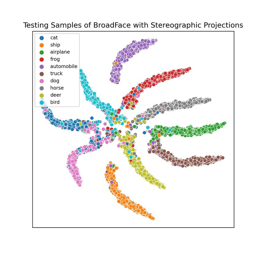
Neural networks which were devised on hyperspherical manifold provided significant performance
compared to standard CNNs [13] [14]. A broad range of objective functions was devised for solving
face verification, face recognition, and similar supervised tasks with hyperspherical intuition. Also,
this intuition is carried by the recent advances in self-supervision by learning features contrastively.
Further, stereographic projection (SP) on hyperspheres is utilized as a pre-processing technique to
understand continuous rotational invariances.
It is observed that erstwhile research (which specifically operates on hyperspherical manifold)
assumes that their objective functions are operated on the hypersphere. But in this work, we utilize
a geometric transformation to map the data points from the euclidean to hyperspherical decision
region. Further, we understand the behavior of angular margin function and standard categorical
cross-entropy (CCE) operated on this manifold.

1.1   Impact of angular margin losses

In recent years various losses have been stated for specific objectives. Rather than learning separable
features, the discriminative approach encourages us to learn features selectively, thus increasing
compactness in intra-class and separability in inter-class features. In discriminative learning, research
has shown that cosine-margin for learned features has significant improvement than euclidean-
margin. Many angular-margin losses have been implemented, specifically for the face recognition
task, based on the analogy that the learned features from a neural network interpret the geometry as a
hyperspherical manifold. Where a margin can control the decision boundary. [12] has developed the
motive of introducing angular constraints to decision functions. Further, [11] has shown normalizing
the weight vectors will advance the [12] with no requirement of joint-supervision by a straightforward
implementation [18] [6] has improved the performance of classifiers by introducing additive-margin
loss function, thus tuning the cosine space and angle space with the margin by rescaling their logits
with a fixed norm. [9] has overcome the problem of mini-batch learning by adding queues to their
framework containing embedding vectors learned from the neural network with their corresponding
identity-representative vector and these vectors are updated throughout training. Although [9] has
utilized the loss function presented in [6], it adopted a new training procedure which has proven
significant improvement in the face recognition dataset.

1.2   Impact on contrastive representation learning

Recently, contrastive representation learning has advanced in deep understanding to learn invariances
both in supervised [8] and self-supervised setting [4]. [19] produced two crucial factors in designing
a contrastive objective function: a) uniformity and b) alignment. These factors played a vital role in
developing a resilient contrastive objective function. While learning representations contrastively, [8]
developed a contrastive loss which was superior to that of self-supervised method [4]. Further, [8]
performed unit sphere normalization to feature sets drawn from an encoder and resulted in outstanding
performance. Both the works focused on training dynamics on unit hypersphere by designing a
contrastive loss.

1.3   Stereographic projections

Closely related work, implementing stereographic projection, was done by [16], [15],and [24].
First, [16] utilized stereographic projection as a pre-processing technique to classify 4-bit parity. The
projection transforms real-valued patterns from one space to another by increasing the dimensionality
and providing superior performance on the two-spiral problem. Where [15], proposed SphereGAN
for image generation problem by utilizing stereographic projection onto hypersphere to attain state-
of-the-art results. [24] tackled with continuity of rotation representations for better training dynamics
of neural networks. The insights of stereographic projections are implied while understanding the
n-dimensional groups with rotations. [21] have utilized stereographic projection as a pre-processing
technique to transform 3D objects to 2D planar images.
The existing research, as mentioned, primarily focused on developing objective functions which
assume that data points lie in the hypersphere. Hence, an appropriate map is not provided to shift the
space and learn invariances from neural networks. Accordingly, we solve this problem by providing a
detailed solution.

                                                   2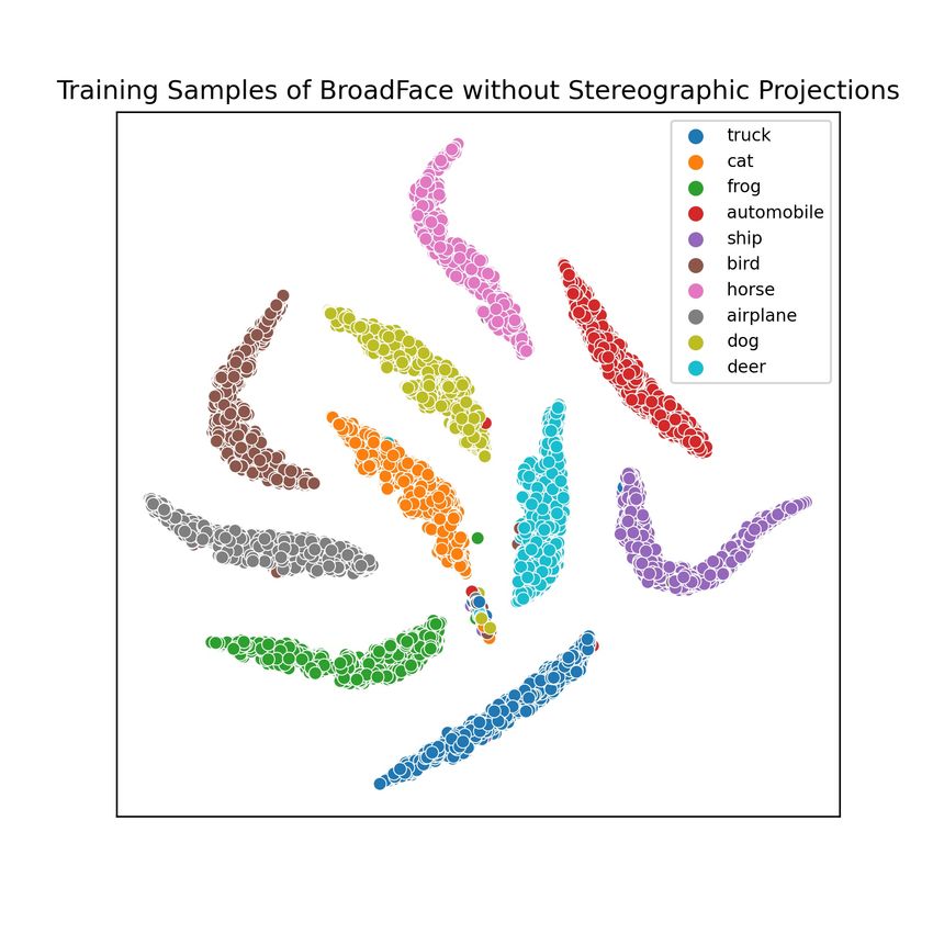
2   Uniqueness of Proposed Work
The uniqueness of our research is twofold.
      1. First, we imply stereographic projection to transform feature vectors from euclidean space
         (Rn ) to hyperspherical manifold (S n ) to analyze the performance of angular margin losses.
      2. Second, proving theoretically and practically that decision boundaries constructed on hyper-
         sphere using stereographic projection oblige the learning of neural networks.

3   Stereographic projection on hyperspherical manifold
Definition Stereographic projection is said to be a map ϕ : Rn = {x ∈ Rn+1 : xn+1 = 0} →
Sn − {en+1 } of x ((n + 1)th dimensional tuple) in euclidean space onto a hypersphere (Sn ) such
that, the x meets a point on hypersphere by linearly extending it till en+1 .
Let ei be a vector in Rn where, ith coordinate is unitary and else are null. Then {e1 , e2 , ..., en } is
orthonormal basis of Rn and also called as standard basis in Rn . So, en+1 is (n + 1)th standard basis
in Rn+1 . So, ϕ(x) is the stereographic projection of x, in euclidean manifold, onto the hyperspherical
manifold. This ϕ(x) lie on the line passing through x and is directed towards en+1 − x. Hence, ϕ(x)
can be written as,
                                    ϕ(x) := x + z ∗ (en+1 − x)                                        (1)
A visual illustration of stereographic projection from R1 → S1 and R2 → S2 is provided for better
intuitiveness in the Fig. 1. Further, there are two underlying key points to be noted while applying
stereographic projection are,
       • The euclidean space (Rn ) must contain the origin.
       • The radius of the hypersphere is unity.
As, ϕ(x) passes through the unit sphere,
                                                            2
                                                 | ϕ(x) | := 1                                       (2)
Substituting equation (1) in (2) results,
                                                                2
                                                        |x| −1
                                                 z :=           2                                    (3)
                                                        |x| +1
Hence, the coordinates obtained after the stereographic projection ϕ of x (x : (x1 , x2 , ..., xn+1 ))
onto hypersphere are,
                                                                              2
                                            2x1             2x2              |x| −1
                          ϕ(x) :=            2      ,           2   , ...,     2                     (4)
                                        |x| +1 |x| +1                        |x| +1

4   Hypersphere as decision region
This section theoretically proves that the hypersphere can be used as a decision region in feed-forward
neural networks. To obtain the transformation from euclidean space (Rn ) to hyperspherical manifold
(Sn ), we imply the earlier described concept stereographic projection.
Theorem 1. A unit hyperspherical manifold Sn is always convex and connected.

Proof. First the convexity and next the connectedness are proven.

Convexity The proof for the convexity of Sn is quite simple [5].
Suppose, x, y ∈ Sn and α ∈ [0, 1].
Using triangle inequality [1],
                || αx + (1 − α)y || ≤ || αx || + || (1 − α)y ||= α + (1 − α) = 1
Hence, αx + (1 − α)y ∈ Sn and thus Sn is convex.

                                                        3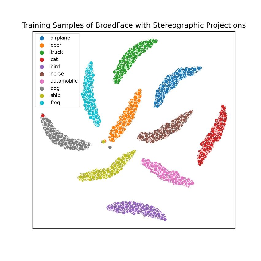
Algorithm 1 PyTorch-like pseudo code for stereographic projection
i/p: input; o/p: output; dim: dimensional ; concat: concatenation; sum: summation; pow(.,2): Squaring the input

#   This function considers (n)-dim i/p vector and returns (n+1)-dim o/p vector.
#   in_vec: input vector
#   norm: norm of in_vec vector
#   a: first n dimensions of the projection
#   b: final dimension of the projection
#   out: stereographic projection

def streographic_preojection (in_vec):
    norm = sum(pow(in_vec,2))
    a = (2*in_vec)/(norm+1)
    b = (norm-1)/(norm+1)
    out = concat(a,b)
    return out

Connectedness To prove this, Sn is equated as union of closed upper hemisphere (Sn+ ) and lower
hemisphere (Sn− ). Individual hemispheres, Sn+ and Sn− are homeomorphic to closed unit disk (Dn ) in
Rn and intersect mutually.
First, let us consider, closed upper hemisphere Sn+ := {u ∈ Rn+1 : un+1 ≥ 0} and the unit disk
Dn := {v ∈ Rn : || v ||≤ 1}. We claim that, Dn shows homeomorphism with Sn+ . The map
f+ : Dn → Sn+ is clearly bijective and continuous. Where,

                                                                     1

                                        Stereographic Projection

                                                        1

                                       Stereographic Projection

Figure 1: Stereographic projections of a point on the real line and a plane are projected onto a circle
and a sphere.

                                                                4
p
f+ (v) := v1 , v2 , ..., vn , 1− || v ||2
As, f+ is a continuous map from a compact topological space to a definite topological space with
homeomorphism. So, in any of the case, Sn+ is connected.
Similarly, it is concluded that, the closed lower hemisphere Sn− := {u ∈ Rn+1 : un+1 ≤ 0} is an
image of f− : Dn → Sn− given by,
p
f− (v) := v1 , v2 , ..., vn , − 1− || v ||2
The observation is clear that the intersection Sn+ ∩ Sn− := {u ∈ Rn+1 : un+1 = 0} is a non-empty
set. Hence, from theorem. 5 (Appendix. 7), we can conclude that Sn is connected.
Proposition 1. A two-layered neural networks decision region possessing the property a) convex
and b) connected aids in decision making by assigning decision boundaries [20]. As unit hypersphere
possess these two properties, and it can be used as a decision region.
Proof. Theorem 1 gives sufficient justification for the above proposition 1.
Thus, ϕ(x) transformation applied at the final layer of the neural networks shifts the decision regions
in Euclidean space to the hyperspherical manifold. As a note, erstwhile research assumed that
data points lie in hyperspherical manifold and devised objective functions. This work removed
this assumption and transformed the data onto a hyperspherical manifold. For a better intuition,
PyTorch-like pseudo-code is explained in Algorithm 1.
5 Experimentation
In this section, a brief introduction to all the angular margin loss functions is provided, as these
loss functions have an underlying assumption that the data points lie in the hypersphere. But, with
stereographic projection, the data points shift their space. So, we analyze that whether stereographic
projections in practicality drive incredible performance for angular margin losses. Subsequently,
the hyperparameters constructed while training the neural network and the training paradigm are
discussed in detail.
5.1 Angular Margin Objectives
First, SphereFace has presented angular-margin Softmax loss(A-Softmax loss), which defines a
decision boundary with a controlled margin. The main task of this loss function is to increase the
posterior probability for the true label by implying the multiplicative angular-margin m between
the learned feature xi and the weight vector Wi of the true label yi . As the margin increases for a
more precise boundary, the constrained region becomes smaller, and the learning task becomes more
problematic. In the below equation weight vector is normalized using L2 normalization. For general
understanding, we replace cosine(.) with ω(.) for feasibility and the original equation is presented in
[11].
!
1 X e||xi ||(ω(mθyi ,i ))
LSphereF ace = − log (5)
N N e||xi ||(ω(mθyi ,i )) + j6=yi e||xi ||(ω(θj,i ))
P
i
CosFace [18] has introduced additive cosine margin as a decision margin. They have normalized the
weight vector Wi and the feature vector xi with L2 normalization and additionally added a scaling
factor s which is the norm of the vector x that is, s = ||x||. Instead of tuning the angle space, it
aims to build a smooth decision boundary and gives reinforcement to the discriminative learning by
tweaking the cosine space with the help of extra margin m. For general understanding,
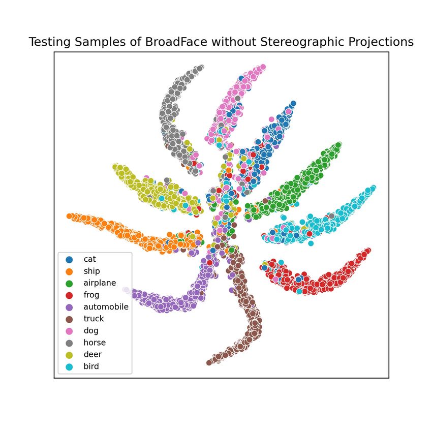
5Figure 2: The above figure illustrates the t-sne embedding of the final decision region (last layer of
neural network). The parameters for t-sne initialized are mentioned in detail. Learning rate ← 200;
perplexity ← 50; iterations ← 1000; angle ← 6 × 10⁻¹ ; initialized with PCA; metric as euclidean;
method for computation is chosen as barrens hut. The number of samples considered to visualize
both train and test is 104 . In the above illustration, considering The train case without projection
confirms a tiny cluster including every (nearly) class, and in a test scenario, they tend to group heavily.
Whereas considering the case of applying stereographic projection, there are fewer samples forming
clusters during training, and there is less affinity to form a cluster in the testing phase.
N
!
1 X es(ω(θyi ,i )−m)
LCosF ace = − log (6)
N i es(ω(θyi ,i )−m) + j6=yi es(ω(θj,i ))
P
ArcFace [6] has introduced additive angular-margin, which has prominent improvement over mul-
tiplicative angular-margin and additive cosine-margin to obtain a precise decision boundary. This
margin is equal to the geodesic distance of the normalized hypersphere [6] also realized the im-
portance of normalization of weight vector Wi and the feature vector xi and added a scaling factor
similar to [18]. Below is the equation of arcface and for better understanding, we replace cos(.) with
6Table 1: The performance analysis of stereographic projection with ResNet as encoder for CIFAR-10
and 100 Data sets. The experiments were implemented five times for variant seeds (fixed batch size).
Where the values are in the mean value, and the deviation is obtained. Data Augmentation is not
implied while training any of the models.
Accuracy(%)
Loss
Datasets Projection applied
Methods
Yes NO
CCE 55.46±0.23 55.65±0.20
SphereFace 59.68±0.15 57.25±0.34
CIFAR-
CosFace 60.71±0.40 57.84±0.41
100
ArcFace 59.65±0.57 58.48±0.42
BroadFace 61.23±0.28 60.29±0.47
CCE 80.92±0.41 81.34±0.15
SphereFace 83.05±0.33 80.78±0.43
CIFAR-
CosFace 84.31±0.32 81.72±0.41
10
ArcFace 84.47±0.34 81.83 ±0.52
BroadFace 85.59±0.24 81.95±0.53
ω(.) in the original equation presented in the equations.
N
!
1 X es(ω(θyi ,i +m))
LArcF ace = − log Pn (7)
N i es(ω(θyi ,i +m)) + j=1,j6=yi es(ω(θj,i ))
BroadFace [9] has adopted the loss function presented in [6] but with an intuitive training procedure,
it has achieved a notable improvement in the face recognition task. For a given [bi ] it supposedly
stores the feature embedding vectors in a queue along with their identity representative vectors Wy i .
Utilizing this past feature embedding vectors present in the queue, it computes loss for the Wy i .
So the neural network has combined loss from the classifier and the embeddings. Embedding loss
is compensated to mitigate the risk from past embedding vectors arisen from b− . To reduce the
additional error, a compensation function is implemented. Below is the equation for BroadFace,
where X is the sample, E is embedding queue, bi is the embedding vector, and b∗j compensated
embedding vector.
1 X X
LBroadF ace = l(bi ) + l(b∗j ) (8)
X ∪E
i∈X j∈E
5.2 Training and Experimentation on CIFAR-10,100
In representation learning, the classification is achieved by extracting representation from an encoder
and performing non-linear mapping with feed-forward neurons. Finally, using a logit function
to classify the patterns. So, we inject stereographic projection as a transformation function to
project latent feature representations onto the hypersphere. This mapping is applied just before the
classification.
During the evaluation, we considered ResNet as our standard baseline encoder [7]. Considering all
the layers would be redundant. Hence architecture pruning is applied [3], [23]. The latent feature
vector, fv obtained by passing through the ResNet encoder and pruning the network by skipping
two pooling layers. Hence, a feature vector fv of shape 4 × 4 × 512 is obtained for standard input
shape of 32 × 32 × 3 (CIFAR-10,100 data). These feature sets were fed into a two-layered, fully
connected dense network with 512, 256 neurons, respectively. The intermediate activations are
typically activated with ReLU. Where ϕ is stereographic projection and utilizing it with angular
margin loss functions at the final layer acts as transformation and eventually acts as a decision
boundary. To understand the representations, t-sne [17] visualizations are provided for the best
performing model (BroadFace) for the CIFAR-10 model with and without projection in Figure 2.
The results obtained in Table 1 depict the performance of stereographic projection on angular margin.
The results are obtained without any augmentation as our aim was to understand the performance
7Table 2: The performance analysis of stereographic projection with ResNet as encoder for malaria
data set. The experiments were implemented five times. Where the values obtained are the mean and
the standard deviation of five variant executions. Data Augmentation is not implied while training
any of the models.
Accuracy(%)
Loss
Datasets Projection applied
Methods
Yes NO
CCE 96.05±1.32 94.91±2.10
Malaria
SphereFace 96.43±2.71 95.48±1.49
Data
BroadFace 96.64±2.48 95.86±2.45
with standard data. Further, the experimentation is conducted five times with random seeds, and the
mean and standard deviations are reported2 .
5.3 Training and Experimentation on Malaria Dataset
The dataset is acquired from the NIH repository3 and consist of two classes: parasitized and uninfected.
Each of the classes has 13,780 images of varying sizes. The complete samples are reshaped into
the identical shape of 128 × 128 × 3. Some of the samples from the dataset are visually depicted
in Figure 3. For evaluation, the training and testing samples were partitioned into 70% and 30% of
complete data, respectively.
Now, in a similar context, ResNet is chosen as encoder [7] and pruning is performed very similarly to
that of previous. Next, SGD is chosen as optimizer (with the momentum of 0.92) with a learning rate
of 10−4 for angular margin objectives. Whereas for CCE, the learning rate is set to 10−3 . The batch
size is the same as that of the previous, and the evaluation has proceeded until it reaches convergence.
As per the results obtained from Table 1, we decided that CosFace and ArcFace are intermediate
models, i.e., their performance is higher than SphereFace and less than that of BroadFace. Hence,
to reduce redundancy, these executions are not considered for the malaria dataset. As the data is
sufficiently large for both classes, we did not perform any augmentation. As previously mentioned,
our goal is to understand the performance of the model with pure data. The results obtained in Table
2 prove the performance of stereographic projection on angular margin objectives and CCE.
6 Disadvantages
Additional Tuning The hyperparameters in angular margin objective functions such as scale factor
and margins are sophisticated to tune. For this, a consistent effort is required to adjust these additional
hyperparameters on variant data sets.
Slower Training During experimentation, we observed that execution time is slightly higher for
the model with stereographic projection than that of the model without projection. This eventually
consumes more electricity, and it is hazardous to the environment.
It should be noted that training and testing samples for CIFAR-10 and 100 are 5 × 10⁴ and 104 respectively.
2
Hence, to plot t-SNE, 104 random training samples and complete testing samples were considered
3
NIH repository (National Library of Medicine) for malaria thin blood smears: Link
Parasitized Uninfected
Figure 3: Sample images of thin blood smear images infected with and without malaria.
87 Conclusion
In this research, we justify theoretically and practically that stereographic projection integrating with
angular margin objective functions for image classification problems improves the decision-making
in neural networks. Instead of assuming the space, it is required to shift the space from euclidean to
hypersphere to provide better performance for standard image classification data as well as malaria
thin blood smear images. In the future, we aim to provide a versatile model that can enhance variant
biomedical tasks’ performance.
References
[1] Stephen Boyd, Stephen P Boyd, and Lieven Vandenberghe. Convex optimization. Cambridge
university press, 2004.
[2] Victor Bryant. Metric spaces: iteration and application. Cambridge University Press, 1985.
[3] Shi Chen and Qi Zhao. Shallowing deep networks: Layer-wise pruning based on feature
representations. IEEE transactions on pattern analysis and machine intelligence, 41(12):3048–
3056, 2018.
[4] Ting Chen, Simon Kornblith, Mohammad Norouzi, and Geoffrey Hinton. A simple framework
for contrastive learning of visual representations. In International conference on machine
learning, pages 1597–1607. PMLR, 2020.
[5] Geir Dahl. An introduction to convexity. University of Oslo, Centre of Mathematics for
Applications, Oslo, Norway, 2010.
[6] Jiankang Deng, Jia Guo, Niannan Xue, and Stefanos Zafeiriou. Arcface: Additive angular
margin loss for deep face recognition. In Proceedings of the IEEE/CVF Conference on Computer
Vision and Pattern Recognition, pages 4690–4699, 2019.
[7] Kaiming He, Xiangyu Zhang, Shaoqing Ren, and Jian Sun. Deep residual learning for image
recognition. In Proceedings of the IEEE conference on computer vision and pattern recognition,
pages 770–778, 2016.
[8] Prannay Khosla, Piotr Teterwak, Chen Wang, Aaron Sarna, Yonglong Tian, Phillip Isola, Aaron
Maschinot, Ce Liu, and Dilip Krishnan. Supervised contrastive learning. In H. Larochelle,
M. Ranzato, R. Hadsell, M. F. Balcan, and H. Lin, editors, Advances in Neural Information
Processing Systems, volume 33, pages 18661–18673. Curran Associates, Inc., 2020.
[9] Yonghyun Kim, Wonpyo Park, and Jongju Shin. Broadface: Looking at tens of thousands
of people at once for face recognition. In European Conference on Computer Vision, pages
536–552. Springer, 2020.
[10] Yann LeCun, Yoshua Bengio, and Geoffrey Hinton. Deep learning. nature, 521(7553):436–444,
2015.
[11] Weiyang Liu, Yandong Wen, Zhiding Yu, Ming Li, Bhiksha Raj, and Le Song. Sphereface:
Deep hypersphere embedding for face recognition. In Proceedings of the IEEE conference on
computer vision and pattern recognition, pages 212–220, 2017.
[12] Weiyang Liu, Yandong Wen, Zhiding Yu, and Meng Yang. Large-margin softmax loss for
convolutional neural networks. In ICML, volume 2, page 7, 2016.
[13] Weiyang Liu, Yan-Ming Zhang, Xingguo Li, Zhiding Yu, Bo Dai, Tuo Zhao, and Le Song.
Deep hyperspherical learning. In I. Guyon, U. V. Luxburg, S. Bengio, H. Wallach, R. Fergus,
S. Vishwanathan, and R. Garnett, editors, Advances in Neural Information Processing Systems,
volume 30. Curran Associates, Inc., 2017.
[14] Pascal Mettes, Elise van der Pol, and Cees Snoek. Hyperspherical prototype networks. Advances
in Neural Information Processing Systems, 32:1487–1497, 2019.
[15] Sung Woo Park and Junseok Kwon. Sphere generative adversarial network based on geometric
moment matching. In Proceedings of the IEEE/CVF Conference on Computer Vision and
Pattern Recognition, pages 4292–4301, 2019.
[16] J Saffery and C Thornton. Using stereographic projection as a preprocessing technique for
upstart. In IJCNN-91-Seattle International Joint Conference on Neural Networks, volume 2,
pages 441–446. IEEE, 1991.
9[17] Laurens van der Maaten and Geoffrey Hinton. Visualizing data using t-sne. Journal of Machine
Learning Research, 9(86):2579–2605, 2008.
[18] Hao Wang, Yitong Wang, Zheng Zhou, Xing Ji, Dihong Gong, Jingchao Zhou, Zhifeng Li, and
Wei Liu. Cosface: Large margin cosine loss for deep face recognition. In Proceedings of the
IEEE conference on computer vision and pattern recognition, pages 5265–5274, 2018.
[19] Tongzhou Wang and Phillip Isola. Understanding contrastive representation learning through
alignment and uniformity on the hypersphere. In International Conference on Machine Learning,
pages 9929–9939. PMLR, 2020.
[20] Alexis Wieland and Russell Leighton. Geometric analysis of neural network capabilities. 1987.
[21] Mohsen Yavartanoo, Eu Young Kim, and Kyoung Mu Lee. Spnet: Deep 3d object classification
and retrieval using stereographic projection. In Asian conference on computer vision, pages
691–706. Springer, 2018.
[22] Matthew D Zeiler and Rob Fergus. Visualizing and understanding convolutional networks. In
European conference on computer vision, pages 818–833. Springer, 2014.
[23] Chenglong Zhao, Bingbing Ni, Jian Zhang, Qiwei Zhao, Wenjun Zhang, and Qi Tian. Varia-
tional convolutional neural network pruning. In Proceedings of the IEEE/CVF Conference on
Computer Vision and Pattern Recognition, pages 2780–2789, 2019.
[24] Yi Zhou, Connelly Barnes, Jingwan Lu, Jimei Yang, and Hao Li. On the continuity of rotation
representations in neural networks. In Proceedings of the IEEE/CVF Conference on Computer
Vision and Pattern Recognition, pages 5745–5753, 2019.
Appendix
In this section, we would like to introduce some basic theorems related to connectedness of a
topological space. These theorems provides an interpretability of Theorem 1.
Theorem 2. A set X in a topological space T is disconnected if X can be written as intersection of
two disjoint, open and non-empty sets. In other cases X is connected.
Proof. The complete proof for this theorem is detailed and elucidated with examples [2].
Theorem 3. The topological space T is connected iff every continuous function f : T → {±1} is
constant.
(or)
Consider a set X, subset of topological space T , is said to be connected if and only if every continuous
function f : X → {±1} is constant.
Proof. Assume, T is not connected.
Therefore, ∃ X, Y ⊂ T are two disjoint and proper non-empty subsets in T . These subsets in are
both open and close in T and T = X ∪ Y .
So, f : T → {±1} can be written as,
+1 , if u∈X
f (u) =
−1 , if u∈Y
Then, f : T → {±1} is a continuous non-constant function. Hence, conversely, the theorem is
proved.
Theorem 4. The topological space T has two connected subsets X, Y such that, X ∩ Y 6= φ. Then,
X ∪ Y is connected,
Proof. Consider, z ∈ X ∩ Y and f : X ∩ Y → {±1} be a continuous function.
∵ X is connected, f is constant on X.
So, f (x) = f (z) ∀ x ∈ X.
10Similarly, f is constant on Y .
So, f (y) = f (z) ∀ y ∈ Y .
From theorem. 4, it can be said that, any continuous function from X ∪ Y to {±1} is constant. Hence,
X ∪ Y is connected.
11You can also read