Improving radar-based rainfall nowcasting by a nearest-neighbour approach - Part 1: Storm characteristics
←
→
Page content transcription
If your browser does not render page correctly, please read the page content below
Hydrol. Earth Syst. Sci., 26, 1631–1658, 2022
https://doi.org/10.5194/hess-26-1631-2022
© Author(s) 2022. This work is distributed under
the Creative Commons Attribution 4.0 License.

Improving radar-based rainfall nowcasting by a nearest-neighbour
approach – Part 1: Storm characteristics
Bora Shehu and Uwe Haberlandt
Institute for Hydrology and Water Resources Management, Leibniz University Hannover, Hanover, Germany

Correspondence: Bora Shehu (shehu@iww.uni-hannover.de)

Received: 6 May 2021 – Discussion started: 10 May 2021
Revised: 17 January 2022 – Accepted: 19 January 2022 – Published: 25 March 2022

Abstract. The nowcast of rainfall storms at fine temporal         the storm dissipation and improves the nowcast compared to
and spatial resolutions is quite challenging due to the un-       the Lagrangian persistence, especially for convective events
predictable nature of rainfall at such scales. Typically, rain-   (storms shorter than 3 h) and longer lead times (from 1 to
fall storms are recognized by weather radar and extrapolated      3 h). The main advantage of the nearest-neighbour approach
in the future by the Lagrangian persistence. However, storm       is seen when applied in a probabilistic way (with the 30 clos-
evolution is much more dynamic and complex than the La-           est neighbours as ensembles) rather than in a deterministic
grangian persistence, leading to short forecast horizons, es-     way (averaging the response from the four closest neigh-
pecially for convective events. Thus, the aim of this paper is    bours). The probabilistic approach seems promising, espe-
to investigate the improvement that past similar storms can       cially for convective storms, and it can be further improved
introduce to the object-oriented radar-based nowcast. Here        by either increasing the sample size, employing more suit-
we propose a nearest-neighbour approach that measures first       able methods for the predictor identification, or selecting
the similarity between the “to-be-nowcasted” storm and past       physical predictors.
observed storms and later uses the behaviour of the past most
similar storms to issue either a single nowcast (by averaging
the 4 most similar storm responses) or an ensemble now-
cast (by considering the 30 most similar storm responses).        1   Introduction
Three questions are tackled here. (i) What features should
be used to describe storms in order to check for similar-         Urban pluvial floods are caused by short, local, and in-
ity? (ii) How should similarity between past storms be mea-       tense rainfall convective storms that overcome rapidly the
sured? (iii) Is this similarity useful for object-oriented now-   drainage capacity of the sewer network and lead to surface
cast? For this purpose, individual storms from 110 events in      inundations. These types of floods are becoming more rele-
the period 2000–2018 recognized within the Hanover Radar          vant with time due to the expansion of urban areas world-
Range (R ∼ 115 km2 ), Germany, are used as a basis for in-        wide (Jacobson, 2011; United Nations, 2018) and the po-
vestigation. A “leave-one-event-out” cross-validation is em-      tential of such storms becoming more extreme under the
ployed to test the nearest-neighbour approach for the predic-     changing global climate (Van Dijk et al., 2014). Because
tion of the area, mean intensity, the x and y velocity com-       of the high economical and even human losses associated
ponents, and the total lifetime of the to-be-nowcasted storm      with these floods, modelling and forecasting becomes cru-
for lead times from + 5 min up to + 3 h. Prior to the applica-    cial for impact-based early warnings (i.e. July 2008 in Dort-
tion, two importance analysis methods (Pearson correlation        mund, Grünewald, 2009, and August 2008 in Tokyo, Kato
and partial information correlation) are employed to iden-        and Maki, 2009). However, one of the main challenges in
tify the most important predictors. The results indicate that     urban pluvial flood forecasting remains the accurate estima-
most of the storms behave similarly, and the knowledge ob-        tion of rainfall intensities at very fine scales. Since the ur-
tained from such similar past storms helps to capture better      ban area responds quickly and locally to the rainfall (due
                                                                  to the sealed surfaces and the artificial deviation of water-

Published by Copernicus Publications on behalf of the European Geosciences Union.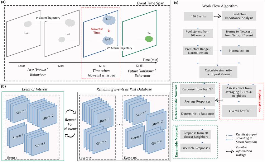
1632                                                 B. Shehu and U. Haberlandt: Improving radar-based rainfall nowcasting

courses), the quantitative precipitation forecasts (QPFs) fed         and extrapolates rainfall structures inside a region together
into the urban models should be provided at very fine tem-            as a unit with a constant velocity (Lucas and Kanade, 1981)
poral (1–5 min) and spatial (100 m2 –1 km2 ) scales (Berne et         and is considered more suitable for major-scale events, i.e.
al., 2004). The numerical weather prediction (NWP) models             stratiform storms, as they are widespread in the radar im-
are typically used in hydrology for weather forecast to sev-          age and exhibit more uniform movements (Han et al., 2009).
eral days ahead; nevertheless, they are not suitable for urban        Even though the field-based approach has gained popularity
modelling as they still cannot produce reliable and accurate          recently (Ayzel et al., 2020; Imhoff et al., 2020), it still has
intensities for spatial scales smaller than 10 km2 and tempo-         trouble nowcasting convective storms. Thus, the focus in this
ral time steps shorter than an hour (Kato et al., 2017; Surcel        study is on object-based nowcasts as they are more conve-
et al., 2015). Ground rainfall measurements (rain gauges) are         nient for convective storms that typically cause urban pluvial
considered the true observation of rainfall, but they are also        floods.
not adequate for QPFs because, due to the sparsity of the                Figure 1 illustrates the three main steps performed in an
existing rain-gauge networks, they cannot capture the spa-            object-based nowcast: (a) first the storm is identified – a
tial structure of rainfall. Therefore, the only product useful in     group of grid cells with intensity higher than a threshold is
providing QPFs for urban pluvial floods remains the weather           recognized in the radar image at time t0 , (b) the storm identi-
radar. The weather radar can measure indirectly the rainfall          fied is then tracked for the time t0 +1t (where 1t is the tem-
intensities at high spatial (∼ 1 km2 ) and temporal (∼ 5 min)         poral resolution of the radar data) and velocities are assigned
resolutions by capturing the reflected energy from the water          from consecutive storm objects, and finally (c) the storm as
droplets in the atmosphere. The rainfall structures and their         lastly observed at time t (when the nowcast is issued) is ex-
evolution in time and space can be easily identified by the           trapolated at a specific lead time (the time in the future when
radar and hence serve as a basis for issuing QPFs at different        the forecast is needed) t+LT , with the last observed velocity
forecast horizons. One of the main drawbacks of radar-based           vector. This is a linear extrapolation of the storm structure in
forecast is that a rainfall structure has to be first identified in   the future considering the spatial structure and the movement
order to be extrapolated in the future. In other words, rain-         of the storm to be constant in time – also referred to as La-
fall cannot be predicted before it has started anywhere in the        grangian persistence (Germann et al., 2006). Applications of
region: only the movement can be predicted. As already dis-           such storm-based nowcasting are common in the literature,
cussed in Bowler et al. (2006) and Jensen et al. (2015), these        like TITAN, HyRaTrac, or Konrad (Han et al., 2009; Hand,
initialization errors cause the radar forecast to be used only        1996; Krämer, 2008; Lang, 2001; Pierce et al., 2004).
for short forecast horizons (up to 3 h), and that is why they            Apart from the initialization errors mentioned before,
are typically referred to as nowcasts. For longer lead times          other error sources in the object-based nowcast can be at-
a blending between NWP and radar-based nowcasts should                tributed to storm identification, storm tracking, and La-
be used instead (Codo and Rico-Ramirez, 2018; Foresti et              grangian extrapolation (Foresti and Seed, 2015; Pierce et al.,
al., 2016; Jasper-Tönnies et al., 2018). Nonetheless, for short       2012; Rossi et al., 2015). Many works have already been con-
forecast horizons up to 2–3 h, the radar nowcast remains the          ducted to investigate the role of different intensity thresholds
best product for pluvial flood simulations as it outperforms          in the storm identification or of different storm-tracking al-
the NWP one (Berenguer et al., 2012; Jensen et al., 2015;             gorithms in the nowcasting results (Goudenhoofdt and De-
Lin et al., 2005; Zahraei et al., 2012).                              lobbe, 2013; Han et al., 2009; Hou and Wang, 2017; Jung and
   Two approaches can be distinguished in the radar-based             Lee, 2015; Kober and Tafferner, 2009). Very-high-intensity
QPFs depending on how the rainfall structures are identi-             thresholds may be suitable for convective storms but can
fied, tracked, and extrapolated into the future: object-oriented      cause false splitting of the storms and can affect negatively
nowcasting (herein referred to as “object-based” to avoid             the tracking algorithm. Thus, one has to be careful when
confusion with the programming term) and field-based now-             adjusting the intensity threshold dynamically over the radar
casting. The object-based nowcast treats rainfall structures as       field and type of storm. A storm-tracking algorithm can be
objects: each object is regarded as a storm and is defined as         improved if certain relationships are learned from past ob-
a set of radar grid cells that moves together as a unit (Dixon        served datasets (like a fuzzy approach in Jung and Lee, 2015,
and Wiener, 1993). The field-based approach considers the             or a tree-based structure in Hou and Wang, 2017), but there is
rainfall to be a continuous field inside a given domain and,          still a limit that the tracking improvement cannot surpass due
through methods like optical flow, tracks and extrapolates            to the implementation of the Lagrangian persistence (Hou
how the intensity moves from one pixel to another inside this         and Wang, 2017). These errors due to the Lagrangian per-
domain (Ruzanski et al., 2011; Zahraei et al., 2012). Con-            sistence are particularly high for convective events at longer
vective storms have been proven to have a unique move-                lead times (past 1 h) as the majority of convective storms
ment from nearby storms (Moseley et al., 2013) and thus               dissipate within 60 min (Goudenhoofdt and Delobbe, 2013;
are thought to be better nowcasted with an object-based ap-           Wilson et al., 1998). At these lead times, the persistence
proach (Kyznarová and Novák, 2009). On the other hand,                fails to predict the dissipation of these storm cells, while for
the field-based approach with an optical flow solution tracks         shorter lead times it fails to represent the growing/decaying

Hydrol. Earth Syst. Sci., 26, 1631–1658, 2022                                          https://doi.org/10.5194/hess-26-1631-2022
B. Shehu and U. Haberlandt: Improving radar-based rainfall nowcasting                                                                    1633

Figure 1. The main steps of an object-based radar nowcast. Blue indicates the current state of the storm at any time t, grey indicates the past
states of the storm (at t0 + 1t), and green indicates the future states of the storm (t0+LT ) (Shehu, 2020).

rate and the changing movement of a storm cell (Germann                   Hou and Wang (2017), where a fuzzy classification scheme
et al., 2006). For stratiform events, since they are more per-            was implemented to improve the tracking and matching of
sistent in nature, Lagrangian persistence can give reliable re-           storms, which resulted in an improved nowcast, and Zahraei
sults up to 2 or 3 h lead time (Krämer, 2008). Nevertheless,              et al. (2013), where a self-organizing-map (SOM) algo-
studies have found that, for fine spatial (1 km2 ) and temporal           rithm was used to predict the initialization and dissipation of
(5 min) scales, the Lagrangian persistence can yield reliable             storms at coarse scales, extending the predictability of storms
results up to 20–30 min lead time, which is also known in the             by 20 %. These studies suggest that past observed relation-
literature as the predictability limit of rainfall at such scales         ships may be useful in extending the predictability limit of
(Grecu and Krajewski, 2000; Kato et al., 2017; Ruzanski et                the convective storms. In this context, a k nearest-neighbour
al., 2011). In object-based radar nowcasting, this predictabil-           method (k-NN) may be developed at the storm scale and
ity limit can be extended up to 1 h for stratiform events and up          used to first recognize similar storms in the past and then
to 30–45 min for convective events if a better radar product              assign their behaviours to the “to-be-nowcasted” storm. The
(merged with rain-gauge data) is fed into the nowcast model               nearest-neighbour method has been used in the field of hy-
(Shehu and Haberlandt, 2021). Past these lead times, the er-              drology, mainly for classification, regression, or resampling
rors due to the growth/decay and dissipation of the storms                purposes (e.g. Lall and Sharma, 1996), but there are some ex-
dominate.                                                                 amples of prediction as well (Galeati, 1990). The assumption
    The predictability of convective storms can be extended               of this method is that similar events are described by similar
if, instead of the Lagrangian persistence, one estimates these            predictors, and if one identifies the predictors successfully,
non-linear processes (growth/decay/dissipation) by utilizing              similar events that behave similarly can be identified. For a
storm life characteristics analysed from past observations                new event, the respective response is then obtained by aver-
(Goudenhoofdt and Delobbe, 2013; Zawadzki, 1973). For                     aging the responses of past k – the most similar storms. The
instance, Kyznarová and Novák (2009) used the CellTrack                   k value can be optimized by minimizing a given cost func-
algorithm to derive life cycle characteristics of convective              tion. Because of the averaging, the response obtained will be
storms and observed that there is a dependency between                    a new one, thus satisfying the condition that nature does not
storm area, maximum intensity, life phase, and height of the              repeat itself, but nevertheless it is confined within the lim-
0 ◦ C isotherm level. Similar results were also found by Mose-            its of the observed events (and therefore is unable to predict
ley et al. (2013), who concluded that convective storms show              extreme behaviours outside of the observed range).
a clear life cycle with the peak occurring at one-third of total             Similar approaches are implemented in field-based now-
storm life, a strong dependency on the temperature, and in-               cast (referred to as analogue events), where past simi-
creasing average intensity with longer durations. In the case             lar radar fields are selected based on weather conditions
of extreme convective storms, earlier peaks are more ob-                  and radar characteristics, i.e. in the NORA nowcast by
vious, causing a steeper increase to maximum intensity. A                 Panziera et al. (2011) mainly for orographic rainfall or in the
later study by Moseley et al. (2019) found that the longest               multi-scaled analogue nowcast model by Zou et al. (2020).
and most intense storms were expected in the late afternoon               Panziera et al. (2011) showed that there is a strong depen-
hours in Germany. Thus, it is to be expected that an exten-               dency between air-mass stability, wind speed and direction,
sive observation of past storm behaviours can be very use-                and the rainfall patterns observed from the radar data and that
ful in creating and establishing new nowcasting rules (Wil-               the NORA nowcast can improve the hourly nowcasts of oro-
son et al., 2010) that can outperform the Lagrangian per-                 graphic rain up to 1 h when compared to Eulerian persistence
sistence. An implementation of such learning from previous                and up to 4 h when compared to the COSMO2 NWP. Im-
observed storms (with focus only on the object-based now-                 provement of predictability through a multi-scaled analogue
cast and not the field-based one) is for instance shown by                nowcast was also reported by Zou et al. (2020), which identi-

https://doi.org/10.5194/hess-26-1631-2022                                               Hydrol. Earth Syst. Sci., 26, 1631–1658, 2022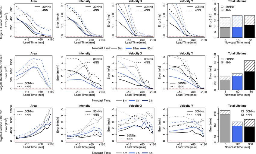
1634                                               B. Shehu and U. Haberlandt: Improving radar-based rainfall nowcasting

fied neighbours first by accounting for similar meteorological     2     Study area and data
conditions and then the spatial information from radar data.
However, both of these studies show the applicability of the       The study area is located in northern Germany and lies within
method to rainfall types that tend to repeat the rainfall pat-     the Hanover Radar Range as illustrated in Fig. 2. The radar
terns, i.e. the orographic forcing in the case of Panziera et      station is situated at Hanover Airport, and it covers an area
al. (2011) and winter stratiform events in the case of Zou et      with a radius of 115 km. The Hanover radar data are C-band
al. (2020). So far, to the authors’ knowledge, such application    data (single-polarization) provided by the German Weather
of the k-NN has not been applied for convective events. This       Service (DWD) and measure the reflectivity at an azimuth
application seems reasonable as an extension of the object-        angle of 1◦ and at 5 min scans (Winterrath et al., 2012).
based radar nowcast in order to treat each convective storm        The reflectivity is converted to intensity according to the
independently. It can be used instead of the Lagrangian per-       Marshall–Palmer relationship with the coefficients a = 256
sistence in step 3 in Fig. 1c for the extrapolation of rainfall    and b = 1.42 (Bartels et al., 2004). The radar data are cor-
storms into the future. Moreover, the benefit of the k-NN ap-      rected from the static clutters and erroneous beams and then
plication is that one can either give a single or an ensemble      converted to a Cartesian coordinate system (1 km2 and 5 min)
nowcast; since k neighbours can be selected as similar to a        as described in Berndt et al. (2014), while the rain gauges
storm at hand, a probability based on the similarity rank can      measure the rainfall intensities at 1 min temporal resolution
be issued at each of the past storms, thus providing an ensem-     but are aggregated to 5 min time steps. Additionally, follow-
ble of responses which are more preferred compared to the          ing the results from Shehu and Haberlandt (2021), a condi-
deterministic nowcast due to the high uncertainty associated       tional merging between the radar data and 100 rain-gauge
with rainfall predictions at such fine scales (Germann and         recordings (see Fig. 2b) with the radar range at 5 min time
Zawadzki, 2004). Thus, it is the aim of this study to inves-       steps is performed. The conditional merging aims to improve
tigate the suitability of the k-NN application for substituting    the kriging interpolation of the gauge recordings by adding
the Lagrangian persistence in the nowcasting of mainly con-        the spatial variability and maintaining the storm structures as
vective events that have the potential to cause urban pluvial      recognized by the radar data. In case a radar image is miss-
floods.                                                            ing, the kriging interpolation of the gauge recordings is taken
   We would like to achieve this by first investigating whether    instead.
a k-NN is able to nowcast successfully storm characteristics          The period from 2000 to 2018 is used as a basis for this
like area, intensity, movement, and total lifetime for differ-     investigation, from which 110 events with different charac-
ent life cycles and lead times. Based on the observed de-          teristics were extracted (see Shehu and Haberlandt, 2021, or
pendency of the storm characteristics on the life cycle, it        Shehu, 2020). These events were selected for urban flood
would be interesting to see whether the morphological fea-         purposes and contain mainly convective events and few strat-
tures are enough to describe the evolution of the convective       iform ones. Here, rainfall events refer to a time period when
storms. Therefore, the focus is here only on the features rec-     rainfall has been observed inside the radar range and at least
ognized by the radar data, and further works will also in-         one rain gauge has registered an extreme rainfall volume (re-
clude the use of meteorological factors. To reach our aim,         turn period higher than 5 years) for durations varying from
the suitability of the k-NN approach is studied as an exten-       5 min to 1 d. The start and the end of the rainfall event are
sion of the existing object-based nowcast algorithm HyRa-          determined when areal mean radar intensity is higher/lower
Trac developed by Krämer (2008). Before such an applica-           than 0.05 mm for more than 4 h. Within a rainfall event many
tion, questions that arise are (I) which features are more im-     rainfall storms, at different times and locations, can be rec-
portant when describing a storm, (II) how to evaluate simi-        ognized. Figure 3a shows a simple illustration to distinguish
larity between storms, and (III) how to use their information      between the rainfall event and rainfall storm concepts em-
for nowcasting the storm at hand. The paper is organized as        ployed in this study.
follows: first, in Sect. 2 the study area is described, followed
by the structure of the k-NN method in Sect. 3.1, where the
                                                                   3     Methods
generation of the storm database is discussed in Sect. 3.1.1,
the predictors selected and target variables in Sect. 3.1.2, the   3.1     Developing the k-NN model
methods used for predictor identification in Sect. 3.1.3, and
different applications of the k-NN in Sect. 3.1.4. The opti-       3.1.1    Generating the storm database
mization and the performance criteria are shown in Sect. 3.2,
followed by the results in Sect. 4 separated into predictor        Each of the selected events contains many storms, whose
influence (Sect. 4.1), deterministic k-NN (Sect. 4.2), prob-       identification and tracking were performed on the basis of the
abilistic k-NN performance (Sect. 4.3), and the nowcasting         HyRaTrac algorithm in the hindcast mode (Krämer, 2008;
of unmatched storms (Sect. 4.4). Finally, the study is ended       Schellart et al., 2014). A storm is initialized if a group of
with conclusions and an outlook in Sect. 5.                        spatially connected radar grid cells (>64) has a reflectivity
                                                                   higher than Z = 20 dBz, while storms are recognized as con-

Hydrol. Earth Syst. Sci., 26, 1631–1658, 2022                                       https://doi.org/10.5194/hess-26-1631-2022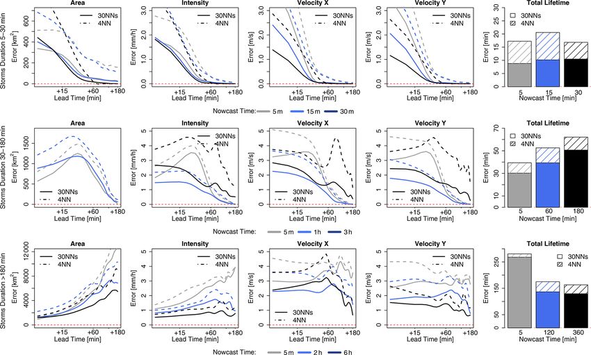
B. Shehu and U. Haberlandt: Improving radar-based rainfall nowcasting                                                               1635

Figure 2. The location of the study area (a) within Germany and (b) with the corresponding elevation and boundaries and with the available
recording rain gauges (purple) and radar station (red). “DEM” is short for “digital elevation model” (adapted from Shehu and Haberlandt,
2021).

vective if a group of bigger than 16 radar grid cells has an           lution the spatial information is saved and various features
intensity higher than 25 dBz and as stratiform if a group of           are calculated. Here the features computed from the spatial
bigger than 128 radar grid cells has an intensity higher than          information of the rainfall inside the storm boundaries at a
20 dBz. Typically, higher values (40 dBz) are used to identify         given time step (in 5 min) of a storm’s life are referred to as
the core of convective storms (as in E-Titan), but to avoid            the “state” of the storm. A storm that has been observed for
false splitting of convective storms and to test the method-           15 min consists of three “states”, each occurring at a 5 min
ology on all types of storms, these identification thresholds          time step. For each of the storm states an ellipsoid is fitted
were kept low (also following the study of Moseley et al.,             to the intensities in order to calculate the major and minor
2013). Once storms at different time steps are recognized,             axes and the orientation angle of the major axis. This storm
they are matched as the evolution of a single storm if the             database is the basis for developing the k-NN method and for
centre of intensity of a storm at t = 0 falls within the bound-        investigating the similarity between storms. Some character-
ary box of the storm at t − 5 min. The tracking of indi-               istics of the identified storms, like duration (or also total life-
vidual storms in consecutive images is done by the cross-              time of the storm), mean area, maximum intensity, number of
correlation optimization between the last two images (t = 0            splits/merges, local velocity components, and ellipsoidal fea-
and t −5 min), and local displacement vectors for each storm           tures, are shown in Fig. 4. These storm characteristics were
are calculated. In case a storm is just recognized (the storm          obtained by a hindcast analysis run of all 110 events with the
does not yet have a previous history), then global displace-           HyRaTrac algorithm, which resulted in around 5200 storms.
ment vectors based on cross-correlation of the entire radar            The local velocities in the x and y directions are obtained
image are assigned to them. It is usually the case that two            by a cross-correlation optimization within the storm bound-
storms merge together at a certain time or that a single storm         ary. The life of the storm is then the lifetime of the radar pixel
splits between several daughter storms. The splitting and              group as dictated by the threshold used to recognize them and
merging of the storms is considered here if two criteria are           the tracking algorithm that decides whether the same storm
met: (a) the minimum distance between the storms that have             is observed at continuous time steps. For more information
split or merged is smaller than the perimeter of the merged            about the tracking and identification algorithm, the reader is
or currently splitting storm and (b) the position of the centre        directed to Krämer (2008).
of intensity of former/latter storms is within the boundaries             As seen from the number of storms for each duration in
of the latter/former storm.                                            Fig. 4, the unmatched storm cells make up the majority of
   Thus, a dataset with several types of storms is built and           the storms recognized. These are storms that last just 5 min
saved. The storms are saved with an ID based on the starting           (one time step), as the algorithm fails to track them at consec-
time and location, and for each time step of the storm evo-            utive time steps. These “storms” can either be dynamic clut-

https://doi.org/10.5194/hess-26-1631-2022                                            Hydrol. Earth Syst. Sci., 26, 1631–1658, 2022

1636                                                  B. Shehu and U. Haberlandt: Improving radar-based rainfall nowcasting

Figure 3. Illustration of concepts and workflows in this study. (a) An event contains many rainfall storms inside the radar range which are
tracked and nowcasted: the dashed grey lines indicate the movements of storms in space and time within the radar event and the event time
span. (b) The “leave-one-out-event cross-validation” – the storms of the event of interest are removed from the past database, and the nowcast
of these storms is issued based on the past database. This process is repeated 110 times (once for each event). (c) The workflow implemented
here for the optimization and application of the k-NN approach.

Figure 4. Different properties of the storms recognized from 110 events separated into six groups according to their duration (shown in
different shades of blue).

Hydrol. Earth Syst. Sci., 26, 1631–1658, 2022                                               https://doi.org/10.5194/hess-26-1631-2022
B. Shehu and U. Haberlandt: Improving radar-based rainfall nowcasting                                                          1637

ter from the radar measurement, as they are characterized by       nowcast (denoted with t0 in Fig. 5) and are calculated from
small areas, circular shapes (small ratios of minor and ma-        one state of the storm. To compute certain features, an el-
jor axes), and very high velocities, or artefacts created by       lipsoid is fitted to each state of the storm. The past features,
low-intensity thresholds used for the storm identification, or     on the other hand, describe the predictors of the past storm
finally produced by the non-representativeness of the volume       states (denoted with t−1 , t−2 in Fig. 5) and their change over
captured by the radar station. Another thing to keep in mind       the past life of the storm. For example, the average area from
is that merged radars are fed to the algorithm for storm recog-    times t−2 to t−1 is a past feature. A pre-analysis of impor-
nition, and this affects the storm structures, particularly when   tant predictors showed that the average features over the last
the radar data are missing. In such a case, the ordinary krig-     30 min are more suitable as past predictors than the averages
ing interpolation of rain gauges is given as the input, which      over the past 15 or 60 min or than the calculation of past
is well known to smoothen the spatial distribution of rainfall     changing rates. Therefore, averages over the past 30 min are
and hence result in a short storm characterized by a very large    computed here:
area. Since the unmatched storms can either be dynamic clut-
ter or artefacts, they are left outside of the k-NN application.           Xt−30 min
                                                                   P30 =               Pi /7,                                    (1)
Nonetheless, they are treated briefly in Sect. 4.5.                           i=t0
   Apart from the unmatched storms, the majority of the re-
maining storms are of a convective nature: storms with short       where Pi is the predictor value at time i and P30 is the av-
duration (shorter than 6 h), high intensity, and low areal cov-    erage value of the predictor over the last 30 min. In case of
erage. Here two types of convective storms are distinguished:      missing values, the remaining time steps are used for aver-
local convective, with very low coverage (on average lower         aging. The selected features (both present and past) that are
than 1000 km2 ) and low intensity (on average ∼ 5 mm h−1 ),        used here to describe storms as objects, and hence tested as
and mesoscale convective, which are responsible for floods         predictors, are shown in Table 1. The present features help
(with intensity up to 100 mm h−1 or more) and have a larger        to recognize storms that are similar at the given state when
coverage (on average lower than 5000 km2 ). The stratiform         the nowcast is issued (blue storm in Fig. 5), and the past ones
storms characterized by large areas, long durations, and low       give additional information about the past evolution of the
intensities as well as meso-γ -scale convective events with        storm (average of grey storms in Fig. 5). The aim of these fea-
durations of up to 6 h are not very well represented by the        tures is to recognize the states of previously observed storms
dataset, as only a few of them are present in the selected         that are most similar to the current one (shown in blue in
events (circa 20 and 50 storms respectively). Therefore, it        Fig. 5) of the to-be-nowcasted storm. Once the most simi-
is to be expected that the k-NN approach will not yield            lar past storm states are recognized, their respective future
very good results for such storms due to the low represen-         states at different lead times can be assigned as the future be-
tativeness. From the characteristics of the storms illustrated     haviour (shown in green in Fig. 5) of the current state of the
in Fig. 4, it can be seen that for stratiform storms that last     to-be-nowcasted storms. Since the storms are regarded as ob-
longer than 12 h the variance of the characteristics is quite      jects with specific features, future behaviours at different lead
low (when compared to the rest of the storms), which can           times are determined by four target variables: area (A+LT ),
be attributed either to the persistence of such storms or to       mean intensity (I+LT ), and velocities in the x (Vx+LT ) and
the low representativeness in the database. Even though the        y (Vy+LT ) directions. Additionally, the total lifetime of the
data size for stratiform storms is quite small, the k-NN may       storm is considered a fifth target (Ltot ). Theoretically, the to-
still deliver good results as characteristics of such storms are   tal lifetime is predicted indirectly when any of the first four
more similar. Nevertheless, the stratiform storms are typi-        targets is set to zero; however, here it is considered an in-
cally nowcasted well by the Lagrangian persistence (espe-          dependent variable in order to investigate whether similar
cially by a field-oriented approach), as they are widespread       storms have similar lifetime durations.
and persistent. Hence the value of the k-NN is primarily seen         For each state of each observed storm in the database, the
for convective storms and not for stratiform ones.                 past and present features of that state with its respective fu-
                                                                   ture states of the five target variables from + 5 to + 180 min
3.1.2   Selecting features for similarity and target               (every 5 min) lead times are saved together and form the
        variables                                                  predictor–target database that is used for the development
                                                                   of the k-NN nowcast model. A summary of the predictors
At first storms are treated like objects that manifest certain     and target variables calculated per state is given in Table
features (predictors) like area, intensity, or lifetime at each    1. Before optimizing and validating the k-NN method (see
state of a storm’s duration until the storm dissipates (and the    Fig. 3c), an importance analysis is performed for each of
predictors are all set to zero). The features of the objects are   the target variables in order to recognize the most important
categorized into present and past features, as illustrated in      predictors. As the predictors have different ranges, prior to
Fig. 5 (shown respectively in blue and grey). The present          the importance analysis and the k-NN application, they are
features describe the current state of the storm at the time of    normalized according to their median and range between the

https://doi.org/10.5194/hess-26-1631-2022                                       Hydrol. Earth Syst. Sci., 26, 1631–1658, 2022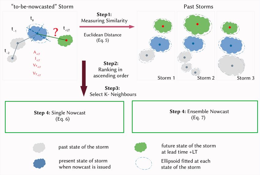
1638                                                    B. Shehu and U. Haberlandt: Improving radar-based rainfall nowcasting

                                                                          a strong linear relationship between them. Here, the Pear-
                                                                          son correlation absolute values are used directly as predictor
                                                                          weights in the k-NN application. However, the relationship
                                                                          between predictors and target variables may still be of a non-
                                                                          linear nature, and thus another predictor importance analy-
                                                                          sis should be recommended when selecting the predictors.
                                                                          Sharma and Mehrotra (2014) proposed a new methodology,
                                                                          designed specifically for the k-NN approach, where no prior
                                                                          assumption about the system type is required. The method is
                                                                          based on a metric called the partial information correlation
                                                                          and is computed from the partial information as
                                                                                  p                             Z
                                                                          PIC = (1 − exp(−2 PI) with PI = fx, P |Z (x, p|z)
Figure 5. The features describing the past (grey) and present (blue)

                                                                                    fx|Z,P |Z (x, p|z)
states of the storm used as predictors to nowcast the future states of      log                            dxdpdz,                   (3)
                                                                                  fx|Z (x|z) fP |Z (p|z)
the storm (green) at a specific lead time (T+LT ) that are described
by four target variables (in red). The nowcast is issued at time t0 . A   where PIC is the partial information correlation and PI is the
full description of these predictors and target variables is given in     partial information which represents the partial dependence
Table 1.
                                                                          of x on P conditioned to the presence of a predictor Z. The
                                                                          partial information itself is a modification of the mutual in-
0.05 and 0.95 quantiles:                                                  formation in order to measure partial statistical dependency
                                                                          between the predictors (P ) and the target variable (x) by
               Pi − Q0.5                                                  adding predictors one at a time (Z) (step-wise procedure).
                     Pi
normPi =                      ,                                    (2)    The evaluation of the PIC needs a pre-existing identified
             Q0.95  0.05
              Pi − QPi                                                    predictor from which the computation can start. If the pre-
                                                                          defined predictor is correctly selected, then, through Eq. (3),
where P is the actual value, normP the normalized value,                  the method is able to recognize and leave out the new predic-
              0.95
and Q0.5                 0.05
        Pi , QPi , and QPi the quantiles 0.5, 0.05, and 0.95              tors which are not related to the response and which do not
of the ith predictor vector. The reason why these quantiles               bring additional value to the existing relationship between
were used for the normalization instead of the typical mean               the current predictors and target variable. Relative weights
and maximum to minimum range is that some outliers are                    for the k-NN regression application can be derived for each
present in the data. For instance, very high and unrealistic              predictor as a relationship between the PIC metric and the
velocities are present in some convective storms where the                associated partial correlation:
tracking algorithm fails to capture adequate velocities (Han
et al., 2009). Thus, to avoid the influence of these outliers,                                    Sx|Z(−j )
                                                                          αj = PICx, Zj |Z(−j )               ,                       (4)
the given range is employed.                                                                      SZj |Z(−j )

3.1.3   Selection of the most relevant predictors                         where x is the target response, Zj is the added predictor
                                                                          from the step-wise procedure, Z(−j ) is the previous pre-
The application of the k-NN method can be relevant if there               dictor vector excluding the predictor Zj , Sx|Z(−j ) are the
is a clear connection between the target variable and the fea-            scaled conditional standard deviations between the target (x)
tures describing this target variable. For instance, in the case          and predictor vector Z(−j ), SZj |Z(−j ) are the scaled condi-
of Galeati (1990), a physical background backed up the con-               tional standard deviations between the additional predictor
nection between the target variable (discharge) and the fea-              (Zj ) and the first predictor vector Z(−j ), and αj is the pre-
tures (daily rainfall volume and mean temperature). In the                dictor weight. R package NPRED was used for the investi-
case of the storms at such fine temporal and spatial scales,              gation of the PIC-derived importance weights (Sharma et al.,
due to the erratic nature of the rainfall itself, there is no phys-       2016).
ically related information that can be extracted from radar                  Here, in this study, these two importance analyses are used
data. Different features of the storm itself can be investi-              to determine the most important predictors and their respec-
gated for their importance to the target variable. Neverthe-              tive weights in the k-NN similarity calculation. For each
less, the identification of such features (referred to here as            target variable the most important predictor identified from
predictors) is difficult because it is bounded to the set of              Pearson correlation is given to the PIC metric as the first pre-
the available data and the relationships considered. Com-                 dictor. The analysis is complex due to the presence of several
monly a strong Pearson correlation between the predictors                 predictors, 38 states of future behaviour for each target vari-
selected and the target variable is used as an indicator of               able (for every 5 min between + 5 and + 180 min lead times),

Hydrol. Earth Syst. Sci., 26, 1631–1658, 2022                                              https://doi.org/10.5194/hess-26-1631-2022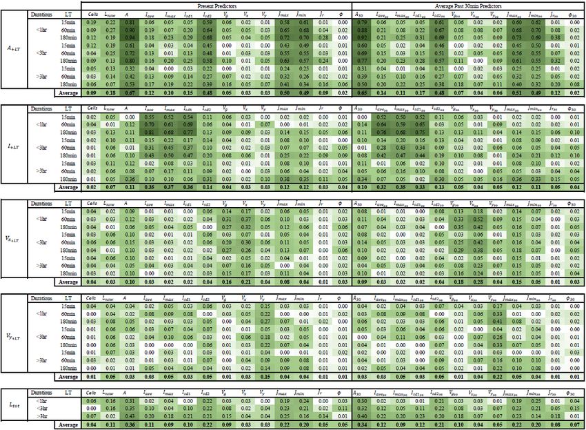
B. Shehu and U. Haberlandt: Improving radar-based rainfall nowcasting                                                        1639

and different nowcast times; the weights were calculated first      according to the rank of the respective neighbour storm:
for three lead times + 15, + 60, and + 180 min and for three
                                                                           (1/Ranki )
storm groups separated according to their durations 3 h. Here the average weights over these                  i=1 (1/Ranki )
groups and lead times are calculated and used as a reference
                                                                    where k is the selected number of neighbours and Rank and
for each importance analysis. The k-NN errors with these av-
                                                                    Pr are respectively the rank and the probability weights of
erage weights are compared in Sect. 4.1.
                                                                    the i neighbour / ensemble member. An ensemble member
3.1.4   Developing the k-NN structure                               is then selected randomly based on the given probability
                                                                    weights. These probability weights calculated here are also
The structure of the proposed k-NN approach at the storm            used for computation of the single nowcast in Eq. (6).
scale is illustrated in Fig. 6 – the current to-be-nowcasted           Since the performance of the single k-NN nowcast is
storm is shown on the left and the past observed storms on          highly dependent on the number of k neighbours used for the
the right. First, in step 1, the Euclidean distance between the     averaging, a prior optimization should be done in order to
most important predictors (either present or past predictors)       select the right k neighbours that yield the best performance
of past storm states and the current one is calculated to iden-     (as illustrated in Fig. 3c). The application of the k-NN can
tify the most similar states of the past storms (distance be-       either be done for each target variable independently or for
tween the blue shapes on the left- and right-hand sides of          all target variables grouped together. In the first approach,
Fig. 6):                                                            the dependency of the target variables between one another
                                                                    is not assured: they are predicted independently of one an-
        r
            XN                                                      other. This is referred to here as the target-based k-NN and
Ed =         i=1
                   wi · (xi − yi )2 ,                        (5)    is denoted in the results as VS1. The main advantage of this
                                                                    application is that, since the relationships between the target
where w is the weight of the respective ith predictor as dic-       variables are not kept, new storms can be generated. Theoret-
tated by the importance analysis (results are shown in Ta-          ically, the predicted variables should have a lower error since
ble 3), x is the predictor of the to-be-nowcasted storm, y is       the application is done separately for each variable; neverthe-
the predictor of a past observed storm, N is the total number       less, this approach does not say much about whether similar
of predictors used, and Ed is the Euclidian distance between        storms behave similarly. Therefore, it is used here as a bench-
the to-be-nowcasted and past observed storms. The assump-           mark for the best possible optimization that can be reached
tion made here is that the smaller the distance, the higher the     by the k-NN with the current selected predictor set. In the
similarity of future behaviour between the selected storms          second approach, the relationships between target variables
and the to-be-nowcasted storm. Therefore, in step 2 these           as exhibited by previous storms are kept. The storm struc-
distances are ranked in ascending order and 30 past storm           ture and the relationship between features are maintained as
states with the smallest distance are selected (step 3). Once       observed, and thus the question of whether similar storms
the similar past storm states have been recognized (the blue        behave similarly can be answered. This is referred to here as
shape in Fig. 6 – right), the future states of these storms (the    the storm-based k-NN and is denoted in the results as VS2.
green shapes in Fig. 6 – right, each for a specific lead time       In this study the two approaches are used (respectively called
from the occurrence of the selected similar blue state) are         VS1 and VS2) to understand the potential and the actual im-
treated as future states (the green shape in Fig. 6 – left) of      provement that the k-NN can bring to the storm nowcast.
the to-be-nowcasted storm. In step 4, either a single (deter-
                                                                    3.2     Application of the k-NN and performance
ministic) or an ensemble (probabilistic) nowcast is issued. If
                                                                            assessment
a single nowcast is selected, then the green instances of the k
neighbours are averaged with weights for each lead time:            3.2.1    Optimizing the deterministic k-NN nowcast
         Xk
Rnew =       i=1
                   Pri · Ri ,                                (6)    The optimization of the k-NN is done based on the
                                                                    5189 storms extracted from 110 events in a “leave-one-out”
where k is the number of neighbours obtained from opti-             cross-validation. Since the unmatched storms can be either
mization, Ri and Pri (from Eq. 7) are respectively the re-          dynamic clutter or artefacts of the tracking algorithm, they
sponse and weight of the ith neighbour, and Rnew is the             are left outside of the k-NN optimization and validation. The
response of the to-be-nowcasted storm as averaged from k            assumption is here that an improvement of the radar data or
neighbours. The response R refers to each of the five target        tracking algorithm would eliminate the unmatched storms,
variables: area, intensity, velocities in the x and y directions,   and hence the focus is only on the improvement that the k-
and total lifetime. By contrast, if a probabilistic nowcast is      NN can introduce to the matched storms. “Leave-one-event-
selected, 30-member ensembles are selected from the clos-           out” cross-validation means here that the storms of each
est 30 storms, where each member is assigned a probability          event have to be nowcasted by considering as a past database

https://doi.org/10.5194/hess-26-1631-2022                                         Hydrol. Earth Syst. Sci., 26, 1631–1658, 2022
1640                                                    B. Shehu and U. Haberlandt: Improving radar-based rainfall nowcasting

Table 1. List of all the past and present features of the storms that are investigated for their importance as predictors, and the respective target
variables calculated for different lead times.

              Features                                                                                          Symbol
 Present      Number of storm cells within the storm region                                                     Cells (–)
 features     Current storm lifetime at time of nowcast                                                         Lnow (min)
              Area of the storm                                                                                 A (km2 )
              Mean spatial intensity                                                                            Iave (mm h−1 )
              Maximum spatial intensity                                                                         Imax (mm h−1 )
              Standard deviation of the spatial intensities                                                     Isd1 (–)
              Standard deviation of intensity groups inside the storm                                           Isd2 (–)
              Global velocity of the entire radar image                                                         Vg (m s−1 )
              x and y components of the local velocity of the storm region                                      Vx , Vy (m s−1 )
              Major and minor axes of the ellipsoid and their ratio                                             Jmax , Jmin (km), Jr (–)
              Orientation angle of the major axis of the ellipsoid                                              8 (◦ )
 Past         Average area over the last 30 min of storm existence                                              A30 (km2 )
 features     Average mean intensity over the last 30 min of storm existence                                    Iave30 (mm h−1 )
              Average maximum intensity over the last 30 min of storm existence                                 Imax30 (mm h−1 )
              Average standard deviation of intensity over the last 30 min of storm existence                   Isd130 (–)
              Average standard deviation of intensity groups over the last 30 min of storm existence            Isd230 (–)
              Average global velocity over the last 30 min of storm existence                                   Vg30 (m s−1 )
              Average x and y components of the local velocity over the last 30 min of storm existence          Vx30 , Vy30 (m s−1 )
              Average value of the major and minor axes of the ellipsoid and their ratio over the last          Jmax30 , Jmin30 (km), Jr30 (–)
              30 min of storm existence
              Average major axis orientation of the ellipsoid over the last 30 min of storm existence           830 (◦ )
 Target       Total lifetime of the storm                                                                       Ltot (min)
 variables    Estimated area and intensity at LT from + 5 to + 180 min                                          A+LT (km2 ), Iave+LT (mm h−1 )
              Estimated velocities x and y at LT from + 5 to + 180 min                                          Vx+LT , Vy+LT (m s−1 )

Figure 6. The main steps involved in the k-NN-based nowcast with the estimation of similar storms (Steps 1 to 3) and assigning the future
responses of past storms as the new response of the “to-be-nowcasted” storm either in a deterministic nowcast (Step 4 – left) or in a
probabilistic nowcast (Step 4 – right).

Hydrol. Earth Syst. Sci., 26, 1631–1658, 2022                                                   https://doi.org/10.5194/hess-26-1631-2022
B. Shehu and U. Haberlandt: Improving radar-based rainfall nowcasting 1641
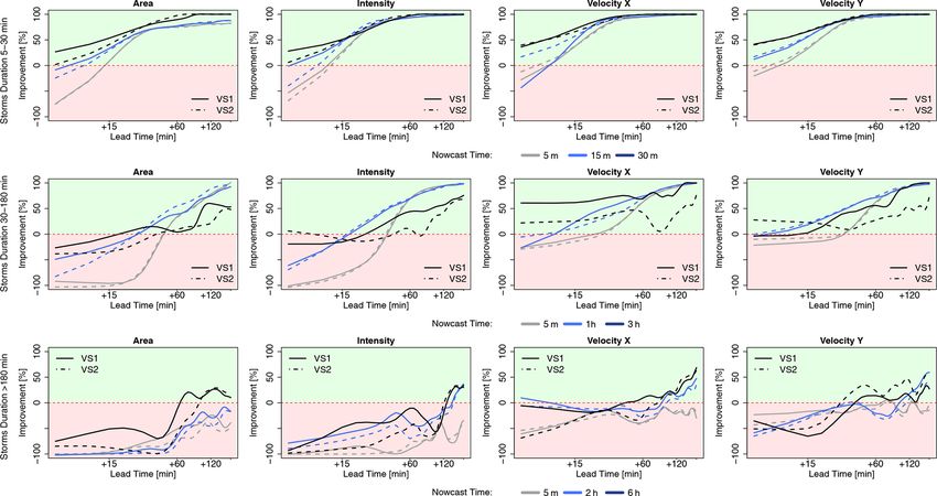
(|Errorref | − |Errornew |)
the storms from the remaining 109 events (a detailed visual- Errorimpr [%] = 100 · , (11)
ization is given in Fig. 3b). The objective function is the mini- |Errorref |
mization of the mean absolute error (MAE) (Eq. 8) and of the where Errornew is the event error manifested by the k-NN,
absolute mean error (ME) (Eq. 9) between predicted and ob- Errorref is the event error manifested by the Lagrangian per-
served target variables at lead times from + 5 to + 180 min: sistence, and Errorimpr is the improvement in reducing the er-
XN ror for each lead time. For improvements higher than 100 %
MAEtarget = i=1
(|Predi, +LT − Obsi,+LT |)/N, (8) or lower than −100 %, the values are reassigned to the limits
XN 100 % and −100 % respectively. Here the Lagrangian persis-
MEtarget = (Predi, +LT − Obsi, +LT )/N , (9)
i=1 tence refers to a persistence of the storm characteristics (area,
where Pred is the predicted response, Obs the observed re- intensity, and velocities in the x and y directions) as last ob-
sponse for the ith storm, +LT the lead time, and N the num- served and constant for all lead times.
ber of storms considered inside an event. The results of the For the probabilistic approach, the continuous rank proba-
storms’ nowcast are also dependent on the nowcast time with bility score (CRPS) as shown in Eq. (12) is computed.
respect to the storms’ life (time step of the storm existence Z∞
when the nowcast is issued – refer to Fig. 3a). If the nowcast
CRPS (F, y) = (F (x) − 1 {y ≤ x} )2 dx
time is 5 min, only the present predictors are used for the cal-
culation of storm similarity and as higher nowcast time as −∞
more predictors are available for the similarity calculation. It 1
= EF |y − y| − EF y − y 0 , (12)
is expected that the nowcast will perform worse in the first 2
5 min of the storm’s existence, as the velocities are not as-
where F is a probabilistic forecast, y is the observed value,
signed properly to the storm region and the past predictors
and y and y 0 are independent random variables with a cumu-
are not yet calculated. Therefore, the optimization is done
lative distribution function (CDF) of F and finite first mo-
separately for three different groups of nowcast times in or-
ment E (Gneiting and Katzfuss, 2014). The CRPS is a gen-
der to achieve a proper application of the k-NN model: Group
eralization of the mean absolute error, and thus if a single
1 – nowcast issued at the first time step of storm recognition,
nowcast is given, it is reduced to the mean absolute error
Group 2 – nowcast issued between 30 min and 1 h of storm
(Eq. 10). This enables a direct comparison between the prob-
evolution, and Group 3 – nowcast issued between 2 and 3 h
abilistic and deterministic nowcasts and an investigation of
of storm evolution. The k number with the lowest absolute
the advantages of the probabilistic one. As in Eq. (8), the
error averaged over all the events for most of the lead times
values obtained in Eqs. (10), (11), and (12) are averaged for
(as the median of MAE from Eq. 9 and ME from Eq. 9 over
each of the 110 events.
all events) is selected as a representative for the deterministic
As stated earlier, the results depend on the nowcast time
nowcast.
and also storm duration (with regard to available storms).
3.2.2 Validating the k-NN deterministic and Therefore, the performance criteria for both k-NN nowcasts
probabilistic nowcasts were computed separately for different storm durations and
nowcast times as illustrated in Table 2. It is important to men-
Once the important predictors are identified and the k-NN tion as well that since one event may contain many storms of
has been optimized, the performance of both deterministic a similar nature, when leaving one event out for the cross-
and probabilistic k-NN is also assessed in a leave-one-event- validation, the number of available storms is actually lower
out cross-validation mode. Two performance criteria are used than the numbers given in Table 2. This particularly affects
to assess the performance. the performance of the storms longer than 6 h, as the leave-
one-event-out cross-validation leaves fewer available storms
i Absolute error per lead time and target variable com-
for the similarity computation. Lastly, it is important to no-
puted for each event and a specific selected nowcast
tice that the performance criteria can be calculated even for
time:
XN nowcast times longer than the storm lifetime if the nowcast
MAEtarget = (|Predi, +LT − Obsi, +LT |)/N, (10) fails to capture the dissipation of the storms. In this case,
i=1
area, intensity, and velocity in the x and y directions are com-
where Pred is the predicted response, Obs is the ob- pared against zero and the total lifetime against the total ob-
served response for the ith storm, +LT is the lead time, served lifetime of the storms.
and N is the number of storms considered inside an
event.
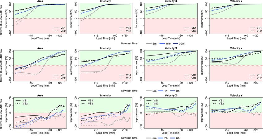
ii The improvement (%) for each lead time and target vari-
able that the k-NN approach introduces to the nowcast
(for a specific selected nowcast time) when compared to
the Lagrangian persistence in an object-based approach:
https://doi.org/10.5194/hess-26-1631-2022 Hydrol. Earth Syst. Sci., 26, 1631–1658, 20221642 B. Shehu and U. Haberlandt: Improving radar-based rainfall nowcasting
Table 2. The selected storm durations and nowcast times for the row), intensity – PIsd1 (as the maximum correlation value
performance calculation of the deterministic and probabilistic now- from the second row), velocity x – Vx30 (as the maximum
casts and the respective number of storms for each case. correlation value from the third row), velocity y – Vy30 (as
the maximum correlation value from the fourth row), and to-
Storm lasting Storms lasting Storms lasting tal lifetime – A (as the maximum correlation value from the
less than 30 min within 0.5–3 h longer than 3 h fifth row). The results of the PIC analysis are shown in the
Nowcast No. of Nowcast No. of Nowcast No. of lower row of Table 3 and in Appendix 11.2. For storm dura-
time storms time storms time storms tion lower than 3 h, where a lot of zeros are present, the PIC
method seems to be unable to converge to stable results or to
5 min 4106 5 min 994 5 min 89
15 min 2265 1h 370 2h 89
identify important predictors. For the intensity and velocity
30 min 271 3h 6 6h 33 components, the PIC identifies only one important predic-
tor, which, in the case of the intensity and velocity in the y
direction, does not correspond to the most important predic-
tor fed first in the analysis. In contrast, for total lifetime and
4 Results area, only for storms that last longer than 3 h is the method
able to converge and give the most important predictors: for
4.1 Predictor importance analysis area – A, Vg, past Vy30 , and Lnow ; for total lifetime – A,
Velg , Lnow , and Jmin30 . At the moment it is unclear why the
Table 3 illustrates the results of the two importance analysis PIC method is unable to perform well for all of the target
methods (Pearson correlation and PIC) for each of the tar- variables and storm groups. One reason might be that only
get variables and their average over the five variables. The the area and total lifetime are dependent on the chosen tar-
stronger the shade of the green colour, the more important get variables. Another most probable reason might be that
is the predictor for the target variable. The weights given for the other target variables the heavy tail of the probabil-
here are averaged from the weights calculated at three dif- ity distribution and the high zero sample size may influence
ferent lead times and storm durations (see Appendices 11.1 the calculation of the joint and mutual probability distribu-
and 11.2 for more detailed information about the calculated tion. The total lifetime is an easier target to be analysed,
weights). First the Pearson correlation weights are recom- which means the values are not zero and its distribution is
mended for the identification of the most important predic- not as heavy tailed as the distribution of the other variables.
tors. From the results it is clear that the autocorrelation has a The other variables, depending on the lead time, have more
higher influence, as the target variables are mostly correlated zeros included and have an asymptotic density function. It
with their respective past and present values. This influence seems that, whenever zeros are not present, like in the case
logically is higher for the shorter lead times and smaller for of storms lasting longer than 3 h, the PIC is able to repre-
the longer lead times. For longer lead times the importance sent quite well the important predictors. However, the reason
increases of other predictors that are not related directly to why this method performs poorly for the application at hand,
the target variable. Similar patterns can be observed among even though developed specifically for the k-NN application,
the area, intensity, and total lifetime target variables, indicat- is not completely understood and is not investigated further
ing that these three variables may be dependent on each other for the time being since it is outside the scope of this paper.
and on similar predictors like current lifetime, area, standard Overall, the results from the Pearson correlation seem
deviation of intensity, the major and minor ellipsoidal axes, more robust and stable (throughout the lead times and storm
and the global velocity. This conclusion agrees well with the groups) than the PIC method (refer to Appendices 11.1 and
life cycle characteristics of convective storms reported in the 11.2); the importance weights increase with the lifetime of
literature review. On the other hand are the velocity compo- the storm and decrease with higher lead time. These be-
nents, which seem to be highly dependent on the autocorrela- haviours are expected, as with increasing lead time the uncer-
tion and slightly correlated with area and the ellipsoidal axes. tainty becomes bigger and with increasing lifetime the storm
It has to be mentioned that, apart from the standard devia- dynamic becomes more persistent (due to the large scales and
tion intensities, also the mean, median, and maximum spatial the stratiform movements involved). Moreover, the impor-
intensities were investigated. Nevertheless, it was found that tant predictors do not change drastically from one lead time
the Isd1 and Isd2 had the higher correlation weights, and since or storm group to the other, as seen in the PIC. Therefore,
there is a high collinearity between these intensity predictors, the predictors estimated from the correlation with the given
they were left out of the predictor’s importance analysis. weights in Table 3 are used as input to the k-NN application.
The application of the PIC analyses requires that the most In order to make sure that the predictor set from the Pearson
important predictors should be introduced to the analysis correlation was the right one, the improvement in the sin-
first. Hence, based on the Pearson correlation values from Ta- gle k-NN training error of using these predictors instead of
ble 3, the following most important predictors were selected: the ones from PIC are shown in Fig. 7. The results shown in
area – A (as the maximum correlation value from the first this figure are computed according to Eq. (11) (where “new”
Hydrol. Earth Syst. Sci., 26, 1631–1658, 2022 https://doi.org/10.5194/hess-26-1631-2022You can also read