Development of a Wilks feature importance method with improved variable rankings for supporting hydrological inference and modelling - HESS
←
→
Page content transcription
If your browser does not render page correctly, please read the page content below
Hydrol. Earth Syst. Sci., 25, 4947–4966, 2021
https://doi.org/10.5194/hess-25-4947-2021
© Author(s) 2021. This work is distributed under
the Creative Commons Attribution 4.0 License.

Development of a Wilks feature importance method with
improved variable rankings for supporting
hydrological inference and modelling
Kailong Li1 , Guohe Huang1 , and Brian Baetz2
1 Faculty   of Engineering, University of Regina, Regina, Saskatchewan, Canada S4S 0A2
2 Department    of Civil Engineering, McMaster University, Hamilton, Ontario, Canada L8S 4L8

Correspondence: Guohe Huang (huangg@uregina.ca)

Received: 1 February 2021 – Discussion started: 1 March 2021
Revised: 31 July 2021 – Accepted: 15 August 2021 – Published: 9 September 2021

Abstract. Feature importance has been a popular approach           1   Introduction
for machine learning models to investigate the relative sig-
nificance of model predictors. In this study, we developed         Machine learning (ML) has been used for hydrological fore-
a Wilks feature importance (WFI) method for hydrologi-             casting and examining modelling processes underpinned
cal inference. Compared with conventional feature impor-           by statistical and physical relationships. Due to the rapid
tance methods such as permutation feature importance (PFI)         progress in data science, increased computational power, and
and mean decrease impurity (MDI), the proposed WFI aims            recent advances in ML, the predictive accuracy of hydrolog-
to provide more reliable variable rankings for hydrological        ical processes has been greatly improved (Reichstein et al.,
inference. To achieve this, WFI measures the importance            2019; Shortridge et al., 2016). Yet, the explanatory power
scores based on Wilks 3 (a test statistic that can be used         of ML models for hydrological inference has not increased
to distinguish the differences between two or more groups of       apace with their predictive power for forecasting (Kona-
variables) throughout an inference tree. Compared with PFI         pala and Mishra, 2020). Previous studies have indicated that
and MDI methods, WFI does not rely on any performance              purely pursuing predictive accuracy may not be a sufficient
measures to evaluate variable rankings, which can thus result      reason for applying a certain hydrological model to a given
in less biased criteria selection during the tree deduction pro-   problem (Beven, 2011). The ever increasing data sources al-
cess. The proposed WFI was tested by simulating monthly            low ML models to incorporate potential driving forces that
streamflows for 673 basins in the United States and applied        cannot be easily considered in physically based hydrolog-
to three interconnected irrigated watersheds located in the        ical models (Kisi et al., 2019). The increasing volume of
Yellow River basin, China, through concrete simulations for        input information has left one challenge as “how to extract
their daily streamflows. Our results indicated that the WFI        interpretable information and knowledge from the model”.
could generate stable variable rankings in response to the re-     Even though obtaining exact mappings from data input to
duction of irrelevant predictors. In addition, the WFI-selected    prediction is technically infeasible for ML models, previous
predictors helped random forest (RF) achieve its optimum           research has shown opportunities to understand the model
predictive accuracy, which indicates that the proposed WFI         decisions through either post hoc explanations or statistical
could identify more informative predictors than other feature      summaries of model parameters (Murdoch et al., 2019). Nev-
importance measures.                                               ertheless, the reliability of the interpretable information is
                                                                   not well understood. Therefore, quality interpretable infor-
                                                                   mation from ML models is much desired for evolving our
                                                                   understanding of nature’s laws (Reichstein et al., 2019).
                                                                      The main idea of model interpretation is to understand the
                                                                   model decisions, including the main aspects of (i) identi-

Published by Copernicus Publications on behalf of the European Geosciences Union.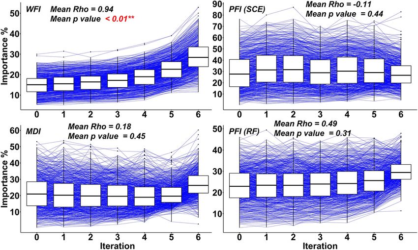
4948                   K. Li et al.: Development of a Wilks feature importance method with improved variable rankings

fying the most relevant predictor variables (i.e. predictors)      rectly (Ribeiro et al., 2016a; Yang, 2020). For instance, the
leading to model predictions and (ii) reasoning why certain        weights (or coefficients) of a linear regression model can
predictors are responsible for a particular model response.        directly reflect how the predictions are produced, thus pro-
Interpretability can be defined as the degree to which a hu-       viding critical information for ranking the model predictors.
man can understand the cause of a decision (Miller, 2019).         Due to the oversimplified input–output relationships, linear
The model interpretation for ML is mainly achieved through         regression models may be inadequate to approximate the
feature importance, which relies on techniques that quan-          complex reality. As a consequence, these models may hardly
tify and rank the variable importance (i.e. a measure of the       achieve satisfactory predictive accuracy and obtain quality
influence of each predictor to predict the output) (Scornet,       interpretable information. As one of the essential branches
2020). The obtained importance scores can be used to ex-           of interpretable models, tree-structured models such as clas-
plain certain predictions through relevant knowledge. More-        sification and regression trees (CART) (Breiman et al., 1984)
over, Gregorutti et al. (2017) pointed out that some irrel-        have been an excellent alternative to linear regression mod-
evant predictors may have a negative effect on the model           els for solving complex non-linear problems. The princi-
accuracy. Therefore, eliminating irrelevant predictors might       ple of CART is to successively split the training data space
improve the predictive accuracy. Feature importance meth-          (i.e. predictors and response) into many irrelevant subspaces.
ods can be categorized as model-agnostic and model-specific        These subspaces and the splitting rules will form a deci-
(Molnar, 2020). The model-agnostic methods refer to ex-            sion/regression tree, which asks each of the new observa-
tracting post hoc explanations by treating the trained model       tions a series of “yes” and “no” questions and guides it to
as a black box (Ribeiro et al., 2016a). Such methods usu-          the corresponding subspaces. The model prediction for a new
ally follow a process of interpretable model learning based        observation shares the same value as the average value for
on the outputs of the black-box model (Craven and Shav-            the training responses in that particular subspace. Mean de-
lik, 1996) and perturbing inputs and seeing the response           crease impurity (MDI) is the feature importance method for
of the black-box model (Ribeiro et al., 2016b). Such meth-         CART, and it summarizes how much a predictor can im-
ods mainly include permutation feature importance (PFI)            prove the model performance through the paths of a tree.
(Breiman, 2001a), partial dependence (PD) plots (Friedman,         Compared with linear regression models, trees are more
2001), individual conditional expectation (ICE) plots (Gold-       understandable for inferring a particular model behaviour
stein et al., 2015), accumulated local effects (ALE) plots         because the transparent decision-making process functions
(Apley and Zhu, 2020), local interpretable model-agnostic          similarly to how the human brain makes decisions for a se-
explanations (LIME) (Ribeiro et al., 2016b), the Morries           ries of questions (Murdoch et al., 2019). Based on CART,
method (Morris, 1991), and Shapley values (Lundberg and            Breiman (2001a) proposed an ensemble of trees named ran-
Lee, 2017; Shapley, 1953). In hydrology, Yang and Chui             dom forest (RF), which significantly improved the predictive
(2020) used Shapley values to explain individual predictions       accuracy compared with CART. Previous studies reported
of hydrological response in sustainable drainage systems at        that RF could outperform many other ML models in predic-
fine temporal scales. Kratzert et al. (2019a) used the Mor-        tive accuracy (Fernández-Delgado et al., 2014; Galelli and
ries method to estimate the rankings of predictors for a long      Castelletti, 2013; Schmidt et al., 2020). The high predictive
short-term memory (LSTM) model. Worland et al. (2019)              accuracy allowed RF to become very useful in interpreta-
used LIME to infer the relation between basin characteris-         tion, especially in hydrology (Lawson et al., 2017; Worland,
tics and the predicted flow duration curves. Konapala and          2018). As Murdoch et al. (2019) argued, higher predictive
Mishra (2020) used partial dependence plots to understand          accuracy can lead to a more reliable inference.
the role of climate and terrestrial components in the devel-          Owing to its widespread success in prediction and inter-
opment of hydrological drought. Compared with the above            pretation, Breiman’s RF has been under active development
model-agnostic methods, PFI is more widely used in hydro-          during the last two decades. For instance, Athey et al. (2019)
logical inference due to its high efficiency and ability to take   presented generalized random forests for solving heteroge-
global insights into model behaviours (Molnar, 2020). Re-          neous estimating equations. Friedberg et al. (2020) proposed
cent applications of PFI include inferring the relationship be-    a local linear forest model to improve the conventional RF
tween basin characteristics and predicted low flow quantiles       in terms of smooth signals. Ishwaran et al. (2008) introduced
(Ahn, 2020) and comparing the interpretability among mul-          random survival forests, which can be used for the analy-
tiple machine learning models in the context of flood events       sis of right-censored survival data. Wager and Athey (2018)
(Schmidt et al., 2020). The above model-agnostic methods           developed a non-parametric causal forest for estimating het-
are useful for comparative studies of ML models with ex-           erogeneous treatment effects (HTE). Du et al. (2021) pro-
ceedingly complex (such as deep neuron networks) algorith-         posed another variant of random forests to help HTE infer-
mic structures to extract the interpretable information.           ence through estimating some key conditional distributions.
   On the other hand, the model-specific methods (also             Katuwal et al. (2020) proposed several variants of heteroge-
known as interpretable models), such as decision trees and         neous oblique random forest employing several linear classi-
sparse regression models, can inspect model components di-         fiers to optimize the splitting point at the internal nodes of the

Hydrol. Earth Syst. Sci., 25, 4947–4966, 2021                                       https://doi.org/10.5194/hess-25-4947-2021
K. Li et al.: Development of a Wilks feature importance method with improved variable rankings                                  4949

tree. These new variants of RF are primarily focused on han-         variable ranking for robust interpretability and optimum pre-
dling various regression and classification tasks or improving       dictive accuracy.
the predictive accuracy; yet their usefulness for interpretation        Therefore, as an extension of the previous efforts, the ob-
has been minimally studied.                                          jective of this study is to develop a Wilks feature importance
   In fact, many studies have reported that the feature im-          (WFI) method with improved variable rankings for support-
portance methods used in Breiman’s RF (including PFI and             ing hydrological inference and modelling. WFI is based on
MDI) are unstable (i.e. a small perturbation of training data        an advanced splitting procedure, stepwise cluster analysis
may significantly change the relative importance of predic-          (SCA) (Huang, 1992), which employed statistical signifi-
tors) (Bénard et al., 2021; Breiman, 2001b; Gregorutti et al.,       cance of the F test, instead of least square fitting (used in
2017; Strobl et al., 2007). Such instability has become one          CART), to determine the optimum splitting points. These
of the critical challenges for the practical use of current fea-     points, in combination with the subsequent sub-cluster mer-
ture importance measures. Yu (2013) defined that statistical         gence, can eventually lead to the desired inference tree for
stability holds if statistical conclusions are robust or stable to   variable rankings. The importance scores of predictors can
appropriate perturbations. In hydrology, stability is critical in    then be obtained according to the values of Wilks 3 for re-
terms of interpretation and prediction. For interpretation, if a     flecting the significance of differences between two or more
distinctive set of variable rankings was observed after a small      groups of response variables. Compared with MDI and PFI,
perturbation of training data, one is unable to conclude re-         WFI does not rely on any performance measures (e.g. least-
alistic reasonings of hydrological processes. For prediction,        square errors in MDI or mean square errors in PFI) and can
there is no guarantee that the predictors with low rankings          thus result in less biased criteria selection during the tree de-
do not bear more valuable information than the higher ones.          duction process. Comparative assessment of WFI, PFI and
This problem challenges the selection of a subset of predic-         MDI performances under the RF framework will then be un-
tors for the optimum predictive accuracy (Gregorutti et al.,         dertaken through efforts in simulating monthly streamflows
2017). Strobl et al. (2008) and Scornet (2020) disclosed the         for 673 basins in the United States. With a finer temporal
finding that positively correlated predictors would lead to          resolution, the proposed approach has also been applied to
biased criteria selection during the tree deduction process,         three irrigated watersheds in the Yellow River basin, China,
which further amplifies such instability. To address the is-         through concrete simulations of their daily streamflows.
sues mentioned above, Hothorn et al. (2006) proposed an
unbiased node splitting rule for criteria selection. The pro-
posed method showed that the predictive performance of               2     Related works
the resulting trees is as good as the performance of estab-
lished exhaustive search procedures used in CART. Strobl et          2.1    Random forest
al. (2007) examined Hothorn’s method under the RF frame-
work, which was called Cforest. They found that the bias of          RF is an ensemble of decision trees, each of which is grown
criteria selection can be further reduced if their method is ap-     in accordance with a random subset of predictors and a boot-
plied using subsampling without replacement. Nevertheless,           strapped version of the training set. As the ensemble mem-
Xia (2009) found that Cforest only outperformed Breiman’s            bers (trees) increase, the non-linear relationships between
RF in some extreme cases and concluded that RF was able              predictors and responses become increasingly stable. The
to provide more accurate predictions and more reliable PFI           prediction can thus be more robust and accurate (Breiman,
compared to Cforest. A similar finding was also achieved             2001a; Zhang et al., 2018). The training set for building each
by Fernández-Delgado et al. (2014), who reported RF was              tree is drawn randomly from the original training dataset with
likely to be the best among 179 ML algorithms (including             replacement. Such bootstrap sampling process will leave
Cforest) in terms of predictive accuracy based on 121 data           about 1/3 of the training dataset as out-of-bag (OOB) data,
sets. More recently, Epifanio (2017) proposed a feature im-          which thus can be used as a validation dataset for the corre-
portance method called intervention in prediction measure            sponding tree.
(IPM), which was reported as a competitive alternative to               There are many variants of RF according to the types of
other PFI and MDI. Since the proposed IPM was specifically           trees (e.g. CART). Based on splitting rules equipped in dif-
designed for high-dimensional problems (i.e. the number of           ferent types of trees, the resulting RF may use various feature
predictors is much larger than the number of observed sam-           importance measures. In this study, Breiman’s RF is selected
ples), it is not suitable for most hydrological problems. Bé-        as the benchmark algorithm to investigate the feature impor-
nard et al. (2021) proposed a stable rule learning algorithm         tance measures. The algorithm is implemented using the R
(SIRUS) based on RF. The algorithm (which aimed to re-               package “randomForest” (Liaw and Wiener, 2002). There are
move the redundant paths of a decision tree) has indicated           three hyperparameters in RF as the number of trees (Ntree),
stable behaviour when data are perturbed, while the predic-          the minimum number of samples in a node (Nmin) for a split-
tive accuracy was not as good as Breiman’s RF. To sum up,            ting action, and the number/ratio of predictors in a subspace
the existing approaches do not guarantee stable and reliable         (Mtry). In addition, Breiman’s RF has two feature importance

https://doi.org/10.5194/hess-25-4947-2021                                         Hydrol. Earth Syst. Sci., 25, 4947–4966, 2021
4950                     K. Li et al.: Development of a Wilks feature importance method with improved variable rankings

Figure 1. The table on the left is a numeric hydrological dataset; the figure on the top right is the tree deduction process for both CART and
SCA with the dataset. (Note that the highlighted numbers in brackets of the leaf nodes are the mean response values of those nodes. In this
particular case, the two algorithms share the same node splitting rules; however, for most real-world cases, they lead to different decision
trees.). The panels on the middle right illustrate the distinct difference of deduction process between CART and SCA (not related to the case);
the table on the bottom right shows the statistic summaries for CART and SCA of this synthetic case.

measures: permutation feature importance (PFI) and mean                   (MSE), given by
decrease impurity (MDI).
                                                                                    1 XN          ∗ 2

                                                                          MSE =        n=1
                                                                                           yn − yn    ,                                         (1)
                                                                                    n
2.2    Permutation feature importance                                     where yn and yn∗ are the nth observed and predicted quanti-
                                                                          ties, respectively, and N is the total number of quantities.
PFI was initially proposed by Breiman (2001a) and can be                  2.3   MDI feature importance
described as follows: assume a trained decision tree t (where
t ∈ {1, . . . , Ntree}; Ntree is the total number of decision trees       The MDI importance measure is based on the CART deci-
in the forest) with a subset of predictor u (where u ∈ p; and             sion tree, which is illustrated using a hydrological dataset
p is complete set of predictors), predictor matrix X (with                (Fig. 1) including 20 instances and 3 predictors as X1 (i.e.
full predictors), response vector Y , predicted vector Y 0 , and          precipitation), X2 (i.e. 3 d cumulative precipitation), and
an error measure L(Y , Y 0 ). (1) Calculate the original model            X 3 (i.e. temperature) and a response Y (i.e. streamflow).
error based on the OOB dataset of the tth decision tree:                  It starts by sorting the value of Xj in ascending order (j
t (eorginal ) = L(Y , t (Xu )) (where Xu is a subset of predictor         indicates the column index of the predictors so that j ∈
matrix X). (2) For each predictor j (where j ∈ {1, . . . , p}), (i)       {1, 2, 3}), and the Y will be reordered accordingly. Then
generate permuted predictor matrix Xperm, j by duplicating X              we go through each instance of Xj from the top to ex-
and shuffling the values of predictor Xj ; (ii) estimate error            amine each candidate split point. For a sample set with k
for the permuted dataset t (eperm, j ) = L(Y , t (Xuperm, j )); and       instances, the total number of split points for Xj will be
(iii) calculate variable importance of predictor j for the tth            k − 1. Any instance z (where z ∈ {1, . . . , k}) in Xj can
decision tree as PFI(t)j = t (eperm, j ) − t (eorginal ); (note that      split the predictor space into two subspaces as X1 (i, j ) =
PFI(t)j = 0 if predictor j is not in u). (3) Calculate the vari-          {x1,j , x2,j , . . . , xz,j } (where i ∈ {1, . . . , z}) and X2 (i, j ) =
able importance for the forest by averaging       the variable im-        {xz+1,j , xz+2,j , . . . , xk,j } (where i ∈ {z + 1, . . . , k}). The re-
                                       1 PNtree
portance over all trees: PFIj = Ntree        t=1 PFI(t) j . The error     sponse space Y will be correspondingly divided into two sub-
measure L(Y , Y 0 ) used in this study is mean squared error              spaces as Y 1 (i) = {y1 , y2 , . . . , yz } (where i ∈ {1, . . . , z}) and

Hydrol. Earth Syst. Sci., 25, 4947–4966, 2021                                                https://doi.org/10.5194/hess-25-4947-2021
K. Li et al.: Development of a Wilks feature importance method with improved variable rankings                                              4951

Y 2 (i) = {yz+1 , yz+2 , . . . , yk } (where i ∈ {z + 1, . . . , k}). To        WFI and MDI comes from the split criterion and the tree de-
maximize the predictive accuracy, the objective of the split-                   duction process. Let us recall the split criterion of CART,
ting process is to find the split point (based on the row and                   in which the optimum split point for Xj is located based
column coordinate z and j , respectively) with the minimum                      on the minimum squared errors of Y 1 and Y 2 as shown in
squared errors (SEs) of Y 1 and Y 2 :                                           Eq. (1). In WFI, this function is achieved by comparing the
                 z                              k
                                                                                two subspaces’ (i.e. Y 1 and Y 2 ) likelihood, which is mea-
                 X                     2       X                    2         sured through the Wilks 3 statistics (Nath and Pavur, 1985;
SE (z, j ) =           Y 1 (i) − Y1         +            Y 2 (i) − Y2 ;
                 i=1                            i=z                             Wilks, 1967). It is defined as 3 = Det(W )/Det(B + W ),
                                                                                where Det(W ) is the determinant of a matrix, and W and
∀ z ∈ 1, . . . , k − 1; ∀ j ∈ 1, . . . , 3,                               (2)
                                                                                B are the within- and between-group sums of squares and
where Y1 and Y2 indicate the mean value of Y 1 and Y 2 , re-                    cross-product matrices in a standard one-way analysis of
spectively.                                                                     variance, respectively. The W and B can be given by
   After each split, each of the newly generated subspaces                         z · (k − z)
can be further split using the same process as long as the                      W=              (Y1 − Y2 )0 · (Y1 − Y2 )                       (5)
                                                                                         k
number of instances in a subspace is greater than a thresh-                        z                                    k−z
old. This process will be repeated until a stopping criterion is
                                                                                   X                 0               X                   0
                                                                                B=      Y 1 (i) − Y1 · Y 1 (i) − Y1 +          Y 2 (i) − Y2
reached, such as a threshold value by which the square errors                        i=1                                   i=1
must be reduced after each split.
                                                                                  · Y 2 (i) − Y2 .
   The importance score of a particular predictor is mea-
                                                                                                                                              (6)
sured based on how effective this predictor can reduce the
square error in Eq. (1) for the entire tree deduction process                   The value of 3 is a measure of how effective X j can differ-
(i.e. MDI). In the case of regression, “impurity” reflects the                  entiate between Y 1 and Y 2 . The smaller 3 value represents
square error of the sample in a subspace (e.g. the larger the                   a larger difference between Y 1 and Y 2 . The distribution of
square error, the more “impure” the subspace is). The de-                       3 is approximated by Rao’s F approximation (R statistic),
crease in node impurity (DI) for splitting a particular space s                 which is defined as
is calculated as
                  X                   2 z                                          1 − 31/S Z · S − d · (m − 1)/2 + 1
DI (z, j, s) =               Y (i) − Y −                                        R=            ·                                               (7)
                                         k                                            31/S            d · (m − 1)
               i∈1,2, ... ,k
                                                                                Z = k − 1 − (d + m)/2                                         (8)
                    X                           2k−z
             ·                   Y 1 (i) − Y1        −                                d 2 · (m − 1)2 − 4
                 i∈1,2, ... ,z
                                                     k                          S=                       ,                                    (9)
                        X                         2                                 d 2 + (m − 1)2 − 5
             ·                        Y 2 (i) − Y2 ,                      (3)
                 i∈z+1,z+2, ... ,k                                              where the R statistic is distributed approximately as an F
                                                                                variate with n1 = d(m − 1) and n2 = d(m − 1)/2 + 1 degrees
where z and j are the coordinates for the optimum splitting                     of freedom, and m is the number of groups. Since the number
point of space s, k is the number of instances in space s, and                  of groups is two in this study, an exact F test is possibly
Y is the mean value of Y (i) in space s. Therefore, the mean                    performed based on the following Wilks 3 criterion as
decrease impurity (MDI) for the variable Xj computed via a
decision tree is defined as                                                                          1−3 k−d −1
                                                                                F (d, k − d − 1) =      ·       .                            (10)
                X                                                                                    3    d
MDI Xj =              Ps · DI(z, j, s),                     (4)
                   s∈S;j =j                                                     Therefore, the two subspaces can be compared for examining
                                                                                significant differences through the F test. The null hypothe-
where S is the total spaces in a tree, and Ps is the fraction
                                                                                sis would be H0 : µ(Y 1 ) = µ(Y 2 ) versus the alternative hy-
of instances falling into s. In other words, the MDI of Xj
                                                                                pothesis H1 : µ(Y 1 ) 6 = µ(Y 2 ), where µ(Y 1 ) and µ(Y 2 ) are
computes the weighted DI related to the splits using the j th
                                                                                population means of Y 1 and Y 2 , respectively. If we let the
predictor. MDI computed via RF is simply the average of the
                                                                                significance level be α, the split criterion would be Fcal
4952 K. Li et al.: Development of a Wilks feature importance method with improved variable rankings
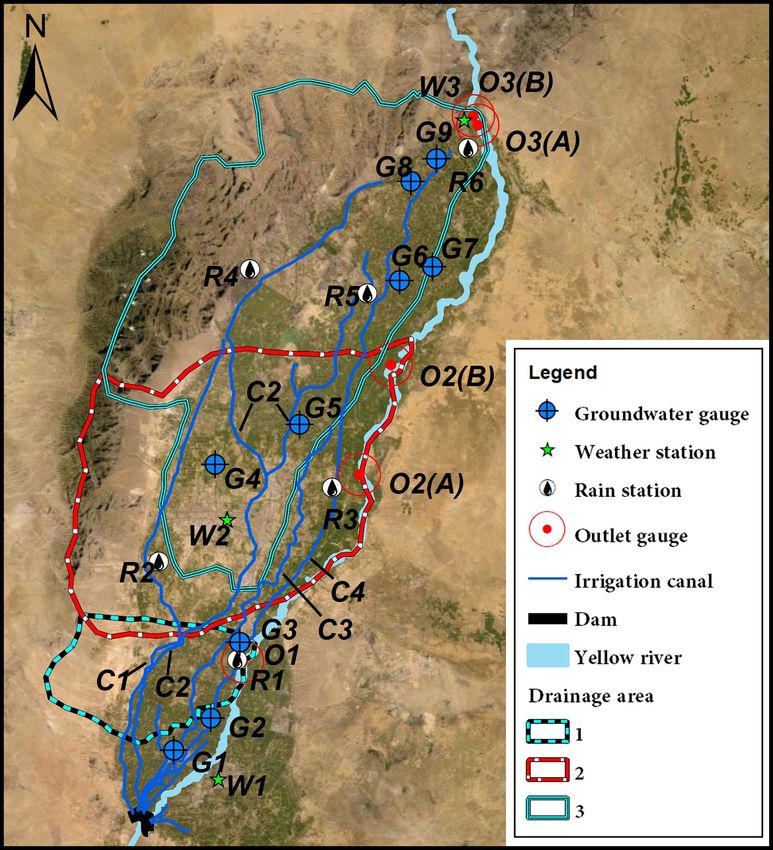
Figure 2. Overview of the basin locations and corresponding hydrological regions. This map was created using ArcGIS software (Esri Inc.
2020).
The merging process will compare any pairs of nodes based nism naturally assumes that the predictors considered (for
on the value of Wilks 3 to test whether they can be merged node splitting) in lower levels of the tree are less signifi-
for Fcal ≥ Fα (H0 is true), which indicates that these two cant than those in upper levels. This effect is even aggra-
subspaces have no significant difference and thus should be vated by the existence of predictor dependence, which will
merged. Such splitting and merging processes are iteratively depress the importance scores of independent predictors and
performed until no node can be further split or merged. Once increase the positively dependent ones (Scornet, 2020). As a
an SCA tree is built, the WFI for the variable Xj computed consequence, some critical predictors may only receive small
via an SCA tree is defined as importance scores. In comparison, Wilks 3 is a measure of
X the separateness of two subspaces, which could avoid the
WFI X j = Ps · (1 − 3(z, j, s)) , (11)
above-mentioned issue for MDI because values of (1 − 3)
s∈S;j =j
do not necessarily decline as long as the tree level goes down
where S is the total spaces in a tree, Ps is the fraction of (as shown in the bottom-right table in Fig. 1). Therefore, the
instances falling into s, and 3 (z, j, s) denotes the value of predictors that are primarily considered in later splits may
3 obtained at the optimum splitting point of space s with have higher importance scores than those in earlier splits. As
row and column coordinates z and j , respectively. Similar to a consequence, some critical predictors might be identified
the calculation of MDI in Eq. (3), the WFI for Xj computes by WFI but overlooked by MDI. Second, the node splitting
the weighted (1 − 3) value related to the splits using the j th mechanism of WFI is based on the F test, which, therefore,
predictor. may significantly reduce the probabilities that the two child
According to the law of large numbers, WFI is expected to nodes are split due to chance. Such a mechanism could be
perform better under the RF framework since the randomized helpful to build more robust input–output relationships for
predictors ensure enough tree diversity, leading to more bal- prediction and inference by reducing overfitting. The above-
anced importance scores. Therefore, we name the ensemble mentioned potential advantages of WFI will be tested with
of SCA as the stepwise clustered ensemble (SCE). In addi- a large number of hydrological simulations in the following
tion to the three hyperparameters (i.e. Ntree, Nmin, and Mtry) two sections.
for Breiman’s RF, SCE also requires the significance level
(α), which is used for the F test during the node splitting
process.
There could be two potential advantages of WFI over
MDI. First, the decrease in node impurity (DI) will become
smaller and smaller as long as the tree level goes down (as
shown in the bottom-right table in Fig. 1). Such a mecha-
Hydrol. Earth Syst. Sci., 25, 4947–4966, 2021 https://doi.org/10.5194/hess-25-4947-2021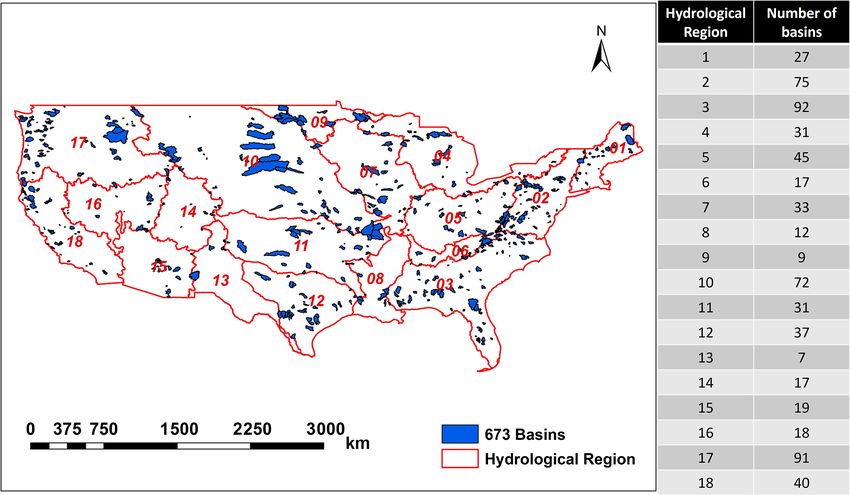
K. Li et al.: Development of a Wilks feature importance method with improved variable rankings 4953
4 Comparative studies over the NCAR CAMELS
dataset
4.1 Dataset description
The Catchment Attributes and Meteorological (CAMELS)
dataset (version 1.2) (Addor et al., 2017; Newman et al.,
2015) was used to evaluate the WFI performance. The dataset
contains daily forcing and hydrologic response data for 673
basins across the contiguous United States that spans a very
wide range of hydroclimatic conditions (Fig. 2) (Newman
et al., 2015). These basins range in size between 4 and
25 000 km2 (with a median basin size of 336 km2 ) and have
relatively low anthropogenic impacts (Kratzert et al., 2019b).
In attempting to demonstrate the relative importance of
meteorological data and large-scale climatic indices on
Figure 3. Adjusted R 2 for 18 hydrological regions. Each box indi-
streamflow, we used monthly mean values of meteorologi- cates statistical summaries (i.e. the bars represent median value; the
cal data in CAMELS dataset and four commonly used large- lower and upper boundaries of a box represent first and third quan-
scale climatic indices (including Nino3.4, Trenberth, 1997; tiles, respectively; dots represent outliers) of adjusted R 2 for all the
Pacific decadal oscillation (PDO), Mantua et al., 1997; in- basins in a particular hydrological region.
terdecadal Pacific oscillation (IPO), Mantua et al., 1997; and
Pacific North American index (PNA), Leathers et al., 1991)
to simulate the monthly streamflows. To reflect the initial
catchment conditions and lagged impact of climatic indices,
the 2-month moving average meteorological data and cli-
matic indices of the preceding 2 months were incorporated as
model predictors. Therefore, the input–output structure (with
22 predictors) for each of these basins can be written as fol-
lows:
P r , Rad , T
maxt , T mint , Vp t , (P r t + P r t−1 ) /2,
t t
(Rad t + Rad t−1) /2, T maxt + T maxt−1 /2,
T
mint + T mint−1 /2, Vp t + Vp t−1 /2,
Qt = f
Nino3.4
t , Nino3.4t−1 , Nino3.4t−2 , P DO t ,
P DO t−1 , P DO t−2 , I P O t , I P O t−1 , I P O t−2 ,
P NAt , P NAt−1 , P NAt−2 , Figure 4. Pairwise comparison for adjusted R2 over 673 US basins.
(12)
where Qt represents streamflow of month t. P r, Rad, T max ,
T min , and Vp represent monthly values of precipitation, repetitions (Molnar, 2020). In this study, the PFI process was
short-wave radiation, maximum temperature, minimum tem- repeated 10 times and then averaged for stabilizing the re-
perature, and vapour pressure, respectively. sults. To facilitate the comparisons among different variable
rankings, importance scores from the three feature impor-
4.2 Evaluation procedures and metrics tance methods were scaled into the [0, 1] range. All the fea-
ture importance methods will be evaluated through recursive
The model training was performed based on January 1980 feature elimination (RFE) (Guyon et al., 2002) as follows:
to December 2005, while the testing was done based on the (1) train SCE and RF models with all predictors; (2) cal-
period of January 2006 to December 2014. The hyperparam- culate the importance scores using the three interpretation
eters for both RF and SCE were set as follows: Ntree was set methods embedded in their corresponding models; (3) ex-
as 100, Nmin was set as 5, and Mtry was set as 0.5 as sug- clude the three least relevant predictors for each set of the
gested by Barandiaran (1998), indicating half of the predic- importance scores obtained in step 2; (4) retrain the models
tors were selected in each tree. In addition, the significance using the remaining predictors in step 3; and (5) repeat step
level (α) was set as 0.05 for the F test in SCE. 2 to 4 until the number of predictors is less than or equal to
The performance of WFI will be evaluated and compared a threshold (set to 4 in this case study). To directly compare
against PFI (applied to RF and SCE) and MDI (applied to the quality of variable rankings from different feature impor-
RF). To improve the stability of the PFI results, previous tance measures, the selected predictors from WFI (after ev-
studies have suggested repeating and averaging the PFI over ery RFE iteration) were also used to train RF. This procedure
https://doi.org/10.5194/hess-25-4947-2021 Hydrol. Earth Syst. Sci., 25, 4947–4966, 2021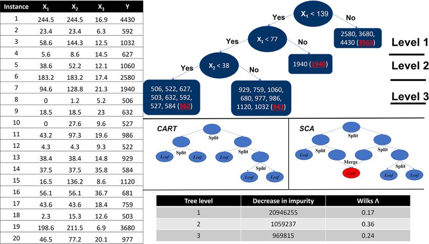
4954                     K. Li et al.: Development of a Wilks feature importance method with improved variable rankings

Figure 5. Iterative change in accuracy in mean values of 673 US basins. The solid lines indicate adjusted R 2 , while the dashed lines represent
RMSE. The panels in the left column show SCE and RF performances based on variables selected by themselves, while the panels on the
right show RF model performances based on variables selected by SCE and RF. The models with an iteration number of 0 represent the
model with all 22 predictors.

allows the effects of different variable rankings to be solely             RMSE is defined as
from feature importance methods (i.e. removed the effects                        v
                                                                                 u N
from different node splitting algorithms). The same proce-                       u1 X             2
dure was also performed for SCE-based PFI (i.e. SCE-PFI)                  RMSE = t        yn − yn∗ ,                                       (14)
                                                                                   n n=1
to examine whether the differences in variable rankings are
from the WFI method or the tree deduction process in SCE.
                                                                          where yn and yn∗ are the nth observed and predicted stream-
   Two error metrics (i.e. adjusted R 2 and RMSE) were used
                                                                          flow values, respectively.
to evaluate the model performance. Adjusted R 2 has been
                                                                             To evaluate the stability of a feature importance method,
used instead of R 2 because adjusted R 2 can consider the
                                                                          we consider reducing predictors during the RFE iterations as
number of predictors. Adjusted R 2 is defined as
                                                                          a form of perturbation to the dataset. Suppose the obtained
               1 − R 2 (N − 1)
                                                                         importance scores for a dominant predictor show an irregu-
     2
adj R = 1 −                      ,                        (13)            lar changing pattern during the RFE iterations. In that case,
                  N −P −1                                                 the method is not stable because it leads to many versions of
where P is the number of predictors, and N is the number of               inferences for such a predictor. On the other hand, if such a
instances.                                                                changing pattern is predictable (e.g. monotonically increas-
                                                                          ing trend), a stable inference can be achieved among interac-
                                                                          tions because the predictable pattern can help analyse how a
                                                                          predictor reacts to the change in the dataset. In this study, the

Hydrol. Earth Syst. Sci., 25, 4947–4966, 2021                                                https://doi.org/10.5194/hess-25-4947-2021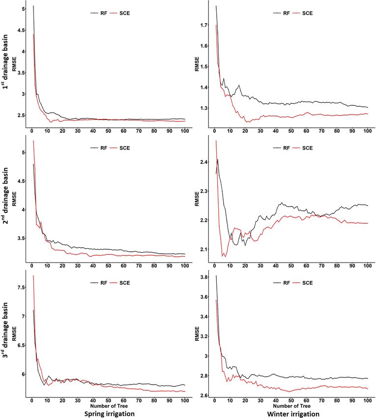
K. Li et al.: Development of a Wilks feature importance method with improved variable rankings                                           4955

Figure 6. Pairwise comparisons of model performance with different feature importance measures. Each of these red points represents the
percentage of basins simulated by model A outperforming model B (based on adjusted R 2 ), in one particular hydrological region. The blue
line represents 50 % percent, and the yellow square represents the mean percentage of 18 hydrological regions.

Figure 7. Pairwise comparisons of RF model performance with different feature importance measures. Z scores and p values are calculated
based on the two-sided Mann–Kendall trend test. If the Z score is greater than 1.96, an increasing trend can be assumed with a significance
level of 0.05. If the Z score is greater than 1.645, an increasing trend can be assumed with a significance level of 0.1. Other notation is the
same as in Fig. 6.

monotonicity is examined using Spearman’s rank correlation                RFE iteration, and RX and RY are the means of RXi and
coefficient (i.e. Spearman’s ρ), which is commonly used to                RYi , respectively. Larger Spearman’s ρ values indicate the
test the statistical dependence between the rankings of two               importance score for a predictor will increase along with the
variables and is defined as                                               reduction of irrelevant predictors, leading to stable impor-
       P                                                                tance scores.
          i RXi − RX RYi − RY
ρ=q                     2          2 ,               (15)
        P
          i RXi − RX       RYi − RY
where RXi denotes the ranks of variables X for the ith RFE
iteration, RYi is the number of selected predictors for the ith

https://doi.org/10.5194/hess-25-4947-2021                                               Hydrol. Earth Syst. Sci., 25, 4947–4966, 2021
4956                     K. Li et al.: Development of a Wilks feature importance method with improved variable rankings

Figure 8. Summaries of the predictors used in the last iterations for 673 US basins.

Figure 9. Mean Spearman’s ρ values for the most important features. The mean p value means how likely it is that the observed correlation
is due to chance. Small p values indicate strong evidence for the observed correlations.

4.3    Predictive accuracy and interpretation stability                  and RF. Therefore, SCA/SCE can be a good substitute for
                                                                         CART/RF.
                                                                            The left column in Fig. 5 shows simulation performances
Figure 3 shows the model testing performances (adjusted R 2 )
                                                                         based on RFE iterations for three feature importance mea-
for 18 hydrological regions with all 22 predictors. The re-
                                                                         sures embedded in SCE and RF. In general, both models can
sults show that SCE and RF significantly outperform SCA
                                                                         improve their simulation performance by eliminating irrele-
and CART, respectively. When taking a close look at these
                                                                         vant predictors. When the number of predictors reduces to
two pairs of model performance, SCA and CART are close
                                                                         7 (i.e. at the 5th iteration), both models reach their highest
to each other, while SCE outperforms RF in most hydrologi-
                                                                         predictive accuracy over the OOB and testing dataset. This
cal regions (except the 9th region).
                                                                         result indicates that it is plausible to use the OOB dataset
   The pairwise comparisons of these four algorithms over
                                                                         to identify the optimum subset of predictors. Comparing the
673 basins show a high coefficient of determination (0.913)
                                                                         simulation performance for the training period, the simula-
of adjusted R 2 between SCE and RF and an even higher
                                                                         tion performance for SCE is much lower than it for RF, while
coefficient of determination (0.965) between SCE and RF
                                                                         an opposite result is observed for the testing period. This re-
(Fig. 4). This result indicates that, in general, it is not likely
                                                                         sult highlights the issue of overfitting for RF. One exception
that there is a distinct performance gap for a particular simu-
                                                                         where RF outperforms SCE (for the testing period) happens
lation task, either between SCA and CART or between SCE

Hydrol. Earth Syst. Sci., 25, 4947–4966, 2021                                             https://doi.org/10.5194/hess-25-4947-2021
K. Li et al.: Development of a Wilks feature importance method with improved variable rankings 4957
in the last (i.e. 6th) iteration, where RF with MDI-selected
predictors outperforms SCE with WFI-selected ones. We can
assume that RF may have a better chance to outperform SCE
with insufficient predictors. Nevertheless, SCE achieves the
overall best performance with PFI-selected predictors.
The upper left panel in Fig. 6 shows that from 0th to 5th it-
erations, over 55 % to 60 % of basins (as indicated by yellow
diamonds) simulated by SCE with WFI-selected predictors
outperform those simulated by RF with MDI-selected pre-
dictors. In comparison, the number drops to about 40 % at
the 6th iteration. This result agrees with the results shown
in Fig. 5. The lower left panel in Fig. 6 shows that from the
1st to 5th iterations, there is a higher chance that SCE with
PFI-selected predictors outperforms RF with MDI-selected
ones for over 75 % of the hydrological regions (as indicated
in Fig. 6 that the black boxes are above the blue line).
The reliability of variable rankings of WFI is further inves-
tigated using the WFI and SCE-PFI-selected predictors from
each of the RFE iterations to run RF models. The results are
shown in the right column in Fig. 5. The RF simulations with
WFI-selected predictors achieved the highest predictive ac-
curacy in most RFE iterations over the training, OOB val-
idation, and testing datasets. In particular, the WFI-selected
predictors have shown significant strength in the last two iter- Figure 10. Map of the study area. Note that due to the extremely
ations and facilitated RF to improve its predictive accuracy. flat surface, three interconnected irrigated watersheds are approxi-
It is worth mentioning that even though SCE-PFI-selected mately delineated. In this map, G indicates groundwater gauges, W
predictors allowed SCE to achieve its optimum performance, indicates weather stations, R indicates rain stations, C indicates ir-
they did not deliver optimum performance for RF. This result rigation canals, and O indicates drainage outlets. Both second and
shows WFI-selected predictors provide a better universal so- third irrigated watersheds contain two cris-crossed drainages with
lution than the PFI-selected ones. strong hydrological connections. The map was created using Ar-
cGIS software (Esri Inc. 2020).
The upper left panel in Fig. 7 shows that the majority of
basins simulated by RF with WFI-selected predictors outper-
form those simulated by RF with MDI-selected predictors.
In particular, at the 6th iteration, basins in 16 (out of 18) hy- ues for monthly precipitation at time step t and t − 1) are
drological regions may own better performance with WFI- considered the two most important predictors for the SCE al-
selected predictors than with the MDI-selected predictors. In gorithm with WFI-selected predictors. In contrast, MDI con-
addition, as the number of predictors decreases, there are in- siders Tmax2 (mean values for the monthly maximum temper-
creasing chances that WFI-selected predictors could generate ature at time step t and t − 1) as the most important predic-
better performance than the MDI-selected ones. Based on a tor for monthly streamflow simulation. It is acknowledged
two-sided Mann–Kendall (M-K) trend test (Kendall, 1948; that streamflow is more responsive to precipitation than air
Mann, 1945), such an increasing trend is significant (i.e. the temperature. Therefore, we can assume that RF may cap-
Z score equals 2.63, and the p value is smaller than 0.01). ture more acute responses of streamflow with WFI-selected
Another significant increasing trend (i.e. the Z score equals predictors than MDI- or PFI-selected ones. This assumption
1.88, and the p value equals 0.06) can also be observed for could be one of the reasons that RF with WFI-selected pre-
the paired studies of WFI and RF-PFI. In contrast, no signif- dictors outperforms the others. It should be noted that IPO
icant increasing trend can be observed for the pairs of SCE- is considered an important predictor for 56 out of 673 basins
PFI and MDI, as well as SCE-PFI and RF-PFI. This finding with WFI, while this predictor has only been employed in 21,
indicates WFI could generate robust variable rankings, based 5, and 10 basins with SCE-PFI, MDI, and RF-PFI methods,
on which informative predictors are more likely to be kept respectively.
for optimum simulation performance. In contrast, other fea- Spearman’s Rho (ρ) values for the predictor with the high-
ture importance measures may lose critical predictors during est importance score (at the last RFE iteration) illustrate the
the RFE process. stability of all three interpretation methods embedded in SCE
Figure 8 shows the summaries of selected predictors (in and RF (Fig. 9). The results indicate that the importance
the last iteration) with different feature importance measures. score for the predominant predictor increases in response to
Pr (monthly precipitation at time step t) and Pr2 (mean val- the reduction of irrelevant predictors. Compared with other
https://doi.org/10.5194/hess-25-4947-2021 Hydrol. Earth Syst. Sci., 25, 4947–4966, 20214958 K. Li et al.: Development of a Wilks feature importance method with improved variable rankings
Figure 11. Convergence of the SCE and RF model based on RMSE over the testing period.
feature importance measures, WFI achieves the highest ρ provides more stable importance scores and will lead to more
values in general, with the p value less than 0.01, indicating a consistent hydrological inferences.
significant correlation between the importance score and the
reduction of irrelevant features. In comparison, eliminating
irrelevant predictors will significantly influence the impor- 5 Application of WFI over irrigated watersheds in the
tance score of predominant predictors obtained by PFI and Yellow River basin, China
MDI. This fact challenges the application of the PFI and MDI
since the removal of irrelevant predictors cannot guarantee 5.1 Study area and data
the same or similar level of hydrological inference because
the importance score may distinctly vary according to the re- Daily streamflow simulations for three irrigated watersheds
duction of irrelevant predictors. In contrast, the WFI method located in the alluvial plain of the Yellow River in China were
conducted to test the capability of the proposed WFI method
Hydrol. Earth Syst. Sci., 25, 4947–4966, 2021 https://doi.org/10.5194/hess-25-4947-2021K. Li et al.: Development of a Wilks feature importance method with improved variable rankings 4959
5.2 Result analysis
Generally, SCE and RF delivered reasonable predictive accu-
racy (using all considered predictors) across all watersheds
and seasons (Table 2). The SCE approaches the best overall
predictive accuracy for the testing dataset. Compared with
RF, the SCE has a smaller drop in predictive accuracy from
the training to testing period, indicating the SCE algorithm
captured a more robust input–output relationship during the
training period. This result agrees with those for the large-
scale dataset in Sect. 4. The convergence tests for training,
OOB validation, and testing datasets were shown in Figs. S1,
S2, and 11, respectively. The results from the testing period
(Fig. 11) show that SCE always outperforms RF as the num-
ber of trees increases.
The iterative reductions in accuracy for training, OOB val-
Figure 12. Change in predictive accuracy averaged across three wa-
idation, and test datasets are listed in Figs. S3, S4, and S5, re-
tersheds and two seasons. Note the change in predictive accuracy
(e.g. RMSE) for a particular case is calculated using (RMSE (last
spectively. The summary (Fig. 12) shows that WFI achieves
iteration) − RMSE (full model)) / RMSE (full model). the smallest reduction in accuracy (for both adjusted R 2 and
RMSE) over the testing period, followed by SCE-PFI, MDI,
and RF-PFI. A smaller reduction in accuracy means the se-
at a finer temporal resolution. These watersheds share a total lected predictors are more informative in describing the com-
area of 4905 km2 , consisting of 52 % irrigated land, 17 % res- plex relationships of hydrological processes. As a conse-
idential area, 15 % desert, 12 % forested land, and 4 % water quence, WFI can identify the most informative predictors
surface (Fig. 10). The landscape of the study area is charac- compared with other methods. Figure 12 also shows that over
terized by an extremely flat surface, with an average slope the training period, RF receives a much smaller impact from
ranging from 1 : 4000 to 1 : 8000, with mostly highly perme- RFE in terms of adjusted R 2 compared with SCE because the
able soil (sandy loam). The climatic condition of the study least-square fittings employed in the CART training process
area is characterized by extreme arid environments, with an- pursue the highest R 2 over the training period.
nual precipitation ranging from 180 to 200 mm and annual Figure 13 shows Spearman’s ρ values for the most relevant
potential evaporation ranging from 1100 to 1600 mm (Yang predictor (i.e. with the highest importance score in the last
et al., 2015). RFE iteration). The result indicates that WFI has the highest
Initial catchment conditions were also considered in this absolute ρ values for the majority of the cases. This result
case study to improve the model performance. Specifically, agrees with the results demonstrated in Sect. 4. In fact, the
moving sums of daily precipitation, temperature, and evap- highest absolute Spearman ρ values for the rest of the rel-
oration time series over multiple time periods δP, T, E = evant predictors (selected for the last RFE iteration) mainly
[1, 3, 5] prior to the date of predictions were set as predic- belong to the WFI method (as shown in Fig. 14), which fur-
tors to reflect the antecedent watershed conditions. Similarly, ther illustrates that WFI could provide stable relative impor-
the moving window for daily irrigation time series was set as tance values for essential predictors for hydrological infer-
δI = [1, 3, 5, 7, 15, 30]. In addition, daily groundwater level ence.
data are used as additional predictors to reflect the baseflow The importance scores were aggregated and analysed ac-
conditions of the catchments. The daily time-series data were cording to different types (i.e. precipitation, irrigation, evap-
divided into two subsets: one from 1 January 2001 to 31 De- oration, etc.) to explore the relationships between the hy-
cember 2011 for model training and OOB validation and the drological responses and their driving forces. We chose the
other from 1 January 2012 to 31 December 2015 for model models with the smallest RMSE (among all the RFE itera-
testing. Table 1 lists the weather, rain, and groundwater sta- tions) on the testing dataset for the hydrological inference.
tions used for each basin. The streamflow processes show The results indicate the importance scores differed signifi-
distinct behaviours in terms of flow magnitude and duration cantly according to the algorithms and interpretation meth-
due to the different irrigation schedules in spring and win- ods used (Fig. 15). In particular, the aggregated predictor
ter. To analyse such temporal variations, daily streamflow P1 (i.e. daily precipitation for time step t from all spatial
for spring–summer (April to September) and autumn–winter locations) achieves positive contributions (in reducing the
(October to March) were examined separately. In this case RMSE) for WFI in the Spring irrigation. At the same time,
study, the hyperparameters for RF and SCE are used the same it has merely no contribution for other feature importance
as in Sect. 4. methods. To investigate whether the predictors identified by
WFI are also meaningful to other algorithms, we reinserted
https://doi.org/10.5194/hess-25-4947-2021 Hydrol. Earth Syst. Sci., 25, 4947–4966, 20214960 K. Li et al.: Development of a Wilks feature importance method with improved variable rankings
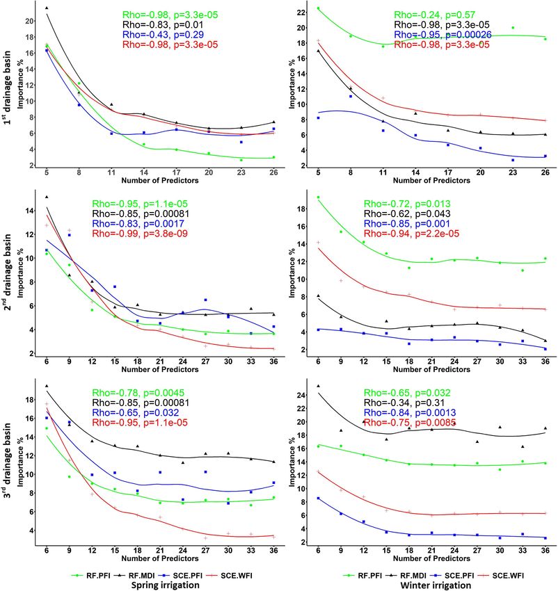
Figure 13. Spearman’s ρ values for the most important predictor. Note that the most important predictor is the predictor with the highest
importance score in the last RFE iteration. The p value means how likely it is that the observed correlation is due to chance. Small p values
indicate strong evidence for the observed correlations.
Table 1. Weather, rain, and groundwater gauges and irrigation canals used in each irrigation basin.
Basin Stations/canals Outlets
First C1, C2, C3, W1, R1, G1, G2, G3 O1
Second C1, C2, C3, C4, W2, R2, R3, R5, G4, G5 O2(A) + O2(B)
Third C1, C2, C4, W2, W3, R4, R5, R6, G4, G5, G6, G7 G8, G9 O3(A) + O3(B)
Note that streamflow for each watershed is integrated as the sum of the gauged streamflows within this area.
Hydrol. Earth Syst. Sci., 25, 4947–4966, 2021 https://doi.org/10.5194/hess-25-4947-2021K. Li et al.: Development of a Wilks feature importance method with improved variable rankings 4961
Table 2. The adjusted R 2 for SCE and RF with all considered predictors.
Basin Season Training OOB Testing
SCE RF SCE RF SCE RF
First spring 94.1 % 98.2 % 86.5 % 88.2 % 82.0 % 81.4 %
First winter 97.9 % 99.2 % 94.3 % 95.1 % 91.3 % 90.0 %
Second spring 94.0 % 98.4 % 85.7 % 89.0 % 76.7 % 75.7 %
Second winter 97.6 % 99.3 % 94.6 % 95.7 % 66.0 % 65.1 %
Third spring 93.8 % 98.3 % 84.5 % 87.7 % 68.5 % 68.1 %
Third winter 97.8 % 99.2 % 95.2 % 95.3 % 82.7 % 82.1 %
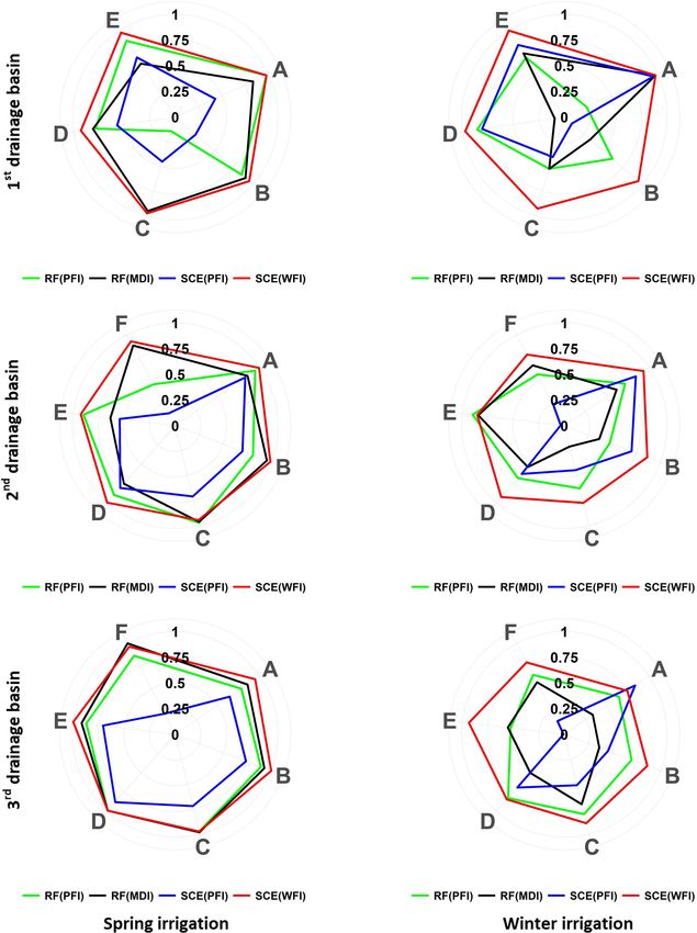
Figure 14. Spearman’s ρ values for three watersheds and seasons. Note that the RFE process of this case study keeps at least five and up to
seven of the most relevant predictors in the last iteration, according to the remainder of the total considered predictors divided by 3. Capital
letters from A to F represent the most relevant predictors identified by different feature importance methods.
https://doi.org/10.5194/hess-25-4947-2021 Hydrol. Earth Syst. Sci., 25, 4947–4966, 20214962 K. Li et al.: Development of a Wilks feature importance method with improved variable rankings
Figure 15. Importance scores aggregated by predictor type. Note that each type of predictor includes predictors from all considered spatial
locations. For example, P1 includes predictors for all the considered climatic stations with 1 d precipitation. Therefore, the importance score
of P1 is the average of the importance score from the predictors of P1.
the predictors in P1 into the best RF model (in which the Table 3. Predictive accuracy for reinserting the predictors in P1 into
set of predictors reaches the smallest RMSE over the testing the RF model (Spring irrigation).
dataset). Indeed, we found the RF with reinserted predictors
showing slightly improved predictive accuracy (i.e. RMSE Basin RF with P1 RF without P1
and adjusted R 2 ) for Spring irrigation across all watersheds RMSE First 2.42 2.44
on the testing dataset (Table 3). This result illustrates that Second 3.16 3.17
even though the predictors in P1 have no contribution in im- Third 5.81 5.81
proving the predictive accuracy on the training dataset, they
can potentially distinguish different hydrological behaviour Adjusted R 2 First 0.81 0.81
Second 0.77 0.76
(i.e. with a small Wilks 3 value) and lead to improved model
Third 0.69 0.69
performance on the testing dataset. In fact, the time of con-
centration for these basins is usually less than 1 d if the storm Note that the RF model was based on the optimum set of predictors in RFE
iterations.
falls near the outlets of the irrigation basins. This fact proves
the above hydrological inference is reasonable.
Hydrol. Earth Syst. Sci., 25, 4947–4966, 2021 https://doi.org/10.5194/hess-25-4947-2021K. Li et al.: Development of a Wilks feature importance method with improved variable rankings 4963
6 Discussion replace those selected by RF with its default methods to im-
prove modelling predictive accuracy.
There could be several reasons why WFI can have more ro- The achievements of the proposed WFI approach are
bust variable rankings than other feature importance mea- twofold: firstly, robust variable rankings are provided for a
sures. First, WFI does not rely on performance measures sound hydrological inference. Specifically, some critical pre-
to evaluate the variable importance. Instead, it depends on dictors that may be overlooked by conventional feature im-
Wilks 3, which prevents any node splitting due to chance. portance methods (PFI and MDI) can be captured through
In the node splitting process, a predictor that significantly in- WFI. Secondly, the enhanced variable rankings combined
creases the predictive accuracy may not necessarily have the with the RFE process can help identify the most important
ability to differentiate two potential subspaces. Therefore, the predictors for optimum model predictive accuracy.
WFI method (which evaluates every splitting and merging The proposed WFI could be a step closer for earth system
action based on Wilks test statistics with the predefined sig- scientists to get a preliminary understanding of the hydro-
nificance level α) is expected to generate more robust vari- logical process through ML. Future studies may focus on the
able rankings. Secondly, WFI considers all the interactions development of tree-structured hydrological models that may
among predictors in the tree deduction process, while PFI can not only be viewed as black-box heuristics, but also can be
only consider the effect of one predictor at a time. Thus the used for rigorous hydrological inference. Even though the fo-
interactions between the target predictor and the rest of the cus of this paper is hydrological inference, WFI can also be
predictors are overlooked. For example, in Sect. 4, the SCE- applied to a variety of other important applications. More-
PFI-selected predictors achieved higher performance (over over, current applications of importance scores are still lim-
the testing dataset) than the WFI-selected ones. However, ited. As interpretable ML continues to mature, its potential
these SCE-PFI-selected predictors are model-specific, which benefits for hydrological inference could be promising.
means when transferring these predictors to the other model
(i.e. RF), they may not deliver the optimum performance. In
contrast, the WFI-selected predictors have good transferabil- Code and data availability. The climatic data are available on the
ity: they helped the RF model achieve optimum predictive data repository of the China Meteorological Data Service Cen-
accuracy. Similar evidence was also found by Schmidt et tre (http://data.cma.cn/en/?r=data/detail&dataCode=A.0012.0001,
al. (2020), who reported that the variable rankings from PFI China Meteorological Data Service Center, 2021). The hydrological
might vary significantly according to different algorithms. data and code for the numeric case can be accessed from the Zen-
odo repository (https://doi.org/10.5281/zenodo.4387068, Li, 2020).
This fact has been considered a major challenge for hydro-
The entire model code for this study can be obtained upon request
logical inference because one cannot reach the same reason- to the corresponding author via email.
ing with different algorithms. Based on the results above, we
can conclude that the WFI could produce more robust vari-
able rankings, which enables a universal solution rather than Supplement. The supplement related to this article is available on-
a specific one for hydrological inference. line at: https://doi.org/10.5194/hess-25-4947-2021-supplement.
RFE was used to identify the most relevant predictors for
optimum predictive accuracy. This approach could be quite
useful in real-world practice, especially in hydrology, where Author contributions. KL designed the research under the supervi-
the simulation problem may involve hundreds of inputs (from sion of GH. KL carried out the research, developed the model code,
climate models, observations, or remote sensing, etc.), de- and performed the simulations. KL prepared the manuscript with
scribing the spatial and temporal variabilities of the system. contributions from GH and BB.
Each of these inputs may contain useful information and may
also contain noise that will mislead the model (e.g. increase
the simulation errors). Therefore, it is critical to eliminate Competing interests. The authors declare that they have no conflict
those variables that cannot improve the predictive accuracy. of interest.
WFI, in combination with the RFE process, can thus be used
for facilitating hydrological inference and modelling.
Disclaimer. Publisher’s note: Copernicus Publications remains
neutral with regard to jurisdictional claims in published maps and
institutional affiliations.
7 Conclusions
WFI was developed to improve the robustness of variable Acknowledgements. We appreciate Ningxia Water Conservancy for
rankings for tree-structured statistical models. Our results in- providing the streamflow, groundwater, and irrigation data, as well
dicate that the proposed WFI can provide more robust vari- as related help. We are also very grateful for the helpful inputs from
able rankings than well-known PFI and MDI methods. In the editor and anonymous reviewers.
addition, we found that the predictors selected by WFI can
https://doi.org/10.5194/hess-25-4947-2021 Hydrol. Earth Syst. Sci., 25, 4947–4966, 2021You can also read