Improving Computational Efficiency in Visual Reinforcement Learning via Stored Embeddings
←
→
Page content transcription
If your browser does not render page correctly, please read the page content below
Improving Computational Efficiency in Visual
                                             Reinforcement Learning via Stored Embeddings

                                                         Lili Chen        Kimin Lee       Aravind Srinivas            Pieter Abbeel
                                                                          University of California, Berkeley
arXiv:2103.02886v1 [cs.LG] 4 Mar 2021

                                                                                       Abstract

                                                 Recent advances in off-policy deep reinforcement learning (RL) have led to im-
                                                 pressive success in complex tasks from visual observations. Experience replay
                                                 improves sample-efficiency by reusing experiences from the past, and convolutional
                                                 neural networks (CNNs) process high-dimensional inputs effectively. However,
                                                 such techniques demand high memory and computational bandwidth. In this paper,
                                                 we present Stored Embeddings for Efficient Reinforcement Learning (SEER), a
                                                 simple modification of existing off-policy RL methods, to address these computa-
                                                 tional and memory requirements. To reduce the computational overhead of gradient
                                                 updates in CNNs, we freeze the lower layers of CNN encoders early in training
                                                 due to early convergence of their parameters. Additionally, we reduce memory
                                                 requirements by storing the low-dimensional latent vectors for experience replay
                                                 instead of high-dimensional images, enabling an adaptive increase in the replay
                                                 buffer capacity, a useful technique in constrained-memory settings. In our experi-
                                                 ments, we show that SEER does not degrade the performance of RL agents while
                                                 significantly saving computation and memory across a diverse set of DeepMind
                                                 Control environments and Atari games. Finally, we show that SEER is useful for
                                                 computation-efficient transfer learning in RL because lower layers of CNNs extract
                                                 generalizable features, which can be used for different tasks and domains.

                                        1   Introduction

                                        Success stories of deep reinforcement learning (RL) from high dimensional inputs such as pixels
                                        or large spatial layouts include achieving superhuman performance on Atari games [32, 39, 1],
                                        grandmaster level in Starcraft II [51] and grasping a diverse set of objects with impressive success
                                        rates and generalization with robots in the real world [23]. Modern off-policy RL algorithms [32,
                                        15, 11, 12, 41, 24, 26] have improved the sample-efficiency of agents that process high-dimensional
                                        pixel inputs with convolutional neural networks (CNNs; LeCun et al. 27) using past experiential data
                                        that is typically stored as raw observations in a replay buffer [30]. However, these methods demand
                                        high memory and computational bandwidth, which makes deep RL inaccessible in several scenarios,
                                        such as learning with much lighter on-device computation (e.g. mobile phones or other light-weight
                                        edge devices).
                                        For compute- and memory-efficient deep learning, several strategies, such as network pruning [13,
                                        8], quantization [13, 18] and freezing [54, 38] have been proposed in supervised learning and
                                        unsupervised learning for various purposes (see Section 2 for more details). In computer vision,
                                        Raghu et al. [38] and Brock et al. [5] showed that the computational cost of updating CNNs can be
                                        reduced by freezing lower layers earlier in training, and Han et al. [13] introduced a deep compression,
                                        which reduces the memory requirement of neural networks by producing a sparse network. In natural
                                        language processing, several approaches [47, 43] have studied improving the computational efficiency
                                        of Transformers [50]. In deep RL, however, developing compute- and memory-efficient techniques
                                        has received relatively little attention despite their serious impact on the practicality of RL algorithms.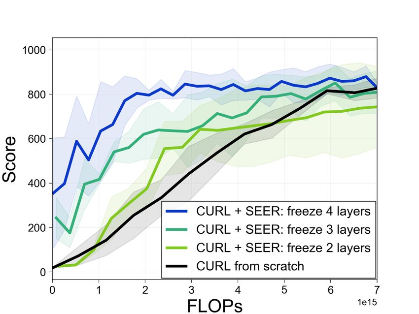
In this paper, we propose Stored Embeddings for Efficient Reinforcement Learning (SEER), a simple
technique to reduce computational overhead and memory requirements that is compatible with various
off-policy RL algorithms [10, 15, 41]. Our main idea is to freeze the lower layers of CNN encoders
of RL agents early in training, which enables two key capabilities: (a) compute-efficiency: reducing
the computational overhead of gradient updates in CNNs; (b) memory-efficiency: saving memory by
storing the low-dimensional latent vectors to experience replay instead of high-dimensional images.
Additionally, we leverage the memory-efficiency of SEER to adaptively increase replay capacity,
resulting in improved sample-efficiency of off-policy RL algorithms in constrained-memory settings.
SEER achieves these improvements without sacrificing performance due to early convergence of
CNN encoders.
The main contributions of this paper are as follows:

    • We present SEER, a compute- and memory-efficient technique that can be used in conjunction
      with most modern off-policy RL algorithms [10, 15].
    • We show that SEER significantly reduces computation while matching the original performance
      of existing RL algorithms on both continuous control tasks from DeepMind Control Suite [46]
      and discrete control tasks from Atari games [2].
    • We show that SEER improves the sample-efficiency of RL agents in constrained-memory settings
      by enabling an increased replay buffer capacity.
    • Finally, we show that SEER is useful for compute-efficient transfer learning, highlighting the
      generality and transferability of encoder features.

2     Related work
Off-policy deep reinforcement learning. The most sample-efficient RL agents often use off-policy
RL algorithms, a recipe for improving the agent’s policy from experiences that may have been
recorded with a different policy [45]. Off-policy RL algorithms are typically based on Q-Learning [52]
which estimates the optimal value functions for the task at hand, while actor-critic based off-policy
methods [29, 40, 10] are also commonly used. In this paper we will consider Deep Q-Networks
(DQN; Mnih et al. 32),which combine the function approximation capability of deep convolutional
neural networks (CNNs; LeCun et al. 27) with Q-Learning along with the usage of the experience
replay buffer [30] as well as off-policy actor-critic methods [29, 10], which have been proposed for
continuous control tasks.
Taking into account the learning ability of humans and practical limitations of wall clock time for
deploying RL algorithms in the real world, particularly those that learn from raw high dimensional
inputs such as pixels [23], the sample-inefficiency of off-policy RL algorithms has been a research
topic of wide interest and importance [25, 22]. To address this, several improvements in pixel-
based off-policy RL have been proposed recently: algorithmic improvements such as Rainbow [15]
and its data-efficient versions [49]; using ensemble approaches based on bootstrapping [36, 28];
combining RL algorithms with auxiliary predictive, reconstruction and contrastive losses [19, 16, 35,
53, 41, 42]; using world models for auxiliary losses and/or synthetic rollouts [44, 9, 22, 12]; using
data-augmentations on images [26, 24].
Compute-efficient techniques in machine learning. Most recent progress in deep learning and RL
has relied heavily on the increased access to more powerful computational resources. To address
this, Mattson et al. [31] presented MLPerf, a fair and precise ML benchmark to evaluate model
training time on standard datasets, driving scalability alongside performance, following a recent
focus on mitigating the computational cost of training ML models. Several techniques, such as
pruning and quantization [13, 8, 4, 18, 47] have been developed to address compute and memory
requirements. Raghu et al. [38] and Brock et al. [5] proposed freezing earlier layers to remove
computationally expensive backward passes in supervised learning tasks, motivated by the bottom-up
convergence of neural networks. This intuition was further extended to recurrent neural networks [33]
and continual learning [37], and Yosinski et al. [54] study the transferability of frozen and fine-tuned
CNN parameters. Fang et al. [7] store low-dimensional embeddings of input observations in scene
memory for long-horizon tasks. We focus on the feasibility of freezing neural network layers in deep
RL and show that this idea can improve the compute- and memory-efficiency of many off-policy
algorithms using standard RL benchmarks.

                                                   2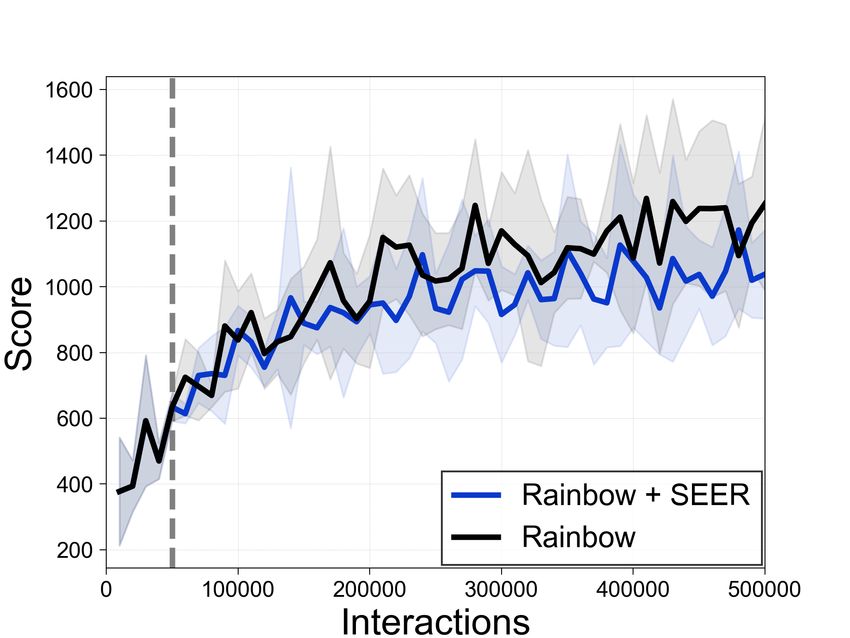
Forward               Actor     Critic              Forward            Actor        Critic
            Backward                                            Backward
                          Latent vector                                                         Latent vector
                            (dim=50)                                                              (dim=50)

                                               Encoder                                             Encoder

          Replay buffer                     3 x 84 x 84       Replay buffer
                (a) SEER before freezing.                            (b) SEER after freezing.
Figure 1: Illustration of our framework. (a) Before the encoder is frozen, all forward and backward
passes are active through the network, and we store images in the replay buffer. (b) After freezing,
we store latent vectors in the replay buffer, and remove all forward and backward passes through the
encoder. We remark that more samples can be stored in the replay buffer due to the relatively low
dimensionality of the latent vector.

3    Background

We formulate visual control task as a partially observable Markov decision process (POMDP; Sutton
& Barto 45, Kaelbling et al. 21). Formally, at each timestep t, the agent receives a high-dimensional
observation ot , which is an indirect representation of the state st , and chooses an action at based on its
policy π. The environment
                   P∞         returns a reward rt and the agent transitions to the next observation ot+1 .
The return Rt = k=0 γ k rt+k is the total accumulated rewards from timestep t with a discount
factor γ ∈ [0, 1). The goal of RL is to learn a policy π that maximizes the expected return over
trajectories. By following the common practice in DQN [32], we handle the partial observability of
environment using stacked input observations, which are processed through the convolutional layers
of an encoder fψ .
Soft Actor-Critic. SAC [10] is an off-policy actor-critic method based on the maximum entropy RL
framework [56], which encourages robustness to noise and exploration by maximizing a weighted
objective of the reward and the policy entropy. To update the parameters, SAC alternates between
a soft policy evaluation and a soft policy improvement. At the soft policy evaluation step, a soft
Q-function, which is modeled as a neural network with parameters θ, is updated by minimizing the
following soft Bellman residual:

           SAC
         LQ (θ, ψ) =Eτt ∼B Qθ (fψ (ot ), at ) − rt

                                                                                         2
                       − γEat+1 ∼πφ Qθ̄ (fψ̄ (ot+1 ), at+1 ) − α log πφ (at+1 |fψ (ot+1 ))     ,

 where τt = (ot , at , rt , ot+1 ) is a transition, B is a replay buffer, θ̄, ψ̄ are the delayed parameters, and
α is a temperature parameter. At the soft policy improvement step, the policy π with its parameter φ
is updated by minimizing the following objective:

                  LSAC
                    π (φ) = Eot ∼B,at ∼πφ α log πφ (at |fψ (ot )) − Qθ (fψ (ot ), at ) .

Here, the policy is modeled as a Gaussian with mean and covariance given by neural networks.
Deep Q-learning. DQN algorithm [32] learns a Q-function, which is modeled as a neural network
with parameters θ, by minimizing the following Bellman residual:
                               "                                                     #
                                                                                 2
             DQN
           L (θ, ψ) = Eτt ∼B Qθ (fψ (ot ), at ) − rt − γ max Qθ̄ (fψ̄ (ot+1 ), a)     ,
                                                                      a

where τt = (ot , at , rt , ot+1 ) is a transition, B is a replay buffer, and θ̄, ψ̄ are the delayed parameters.
Rainbow DQN integrates several techniques, such as double Q-learning [48] and distributional
DQN [3]. For exposition, we refer the reader to Hessel et al. [15] for more detailed explanations of
Rainbow DQN.

                                                          3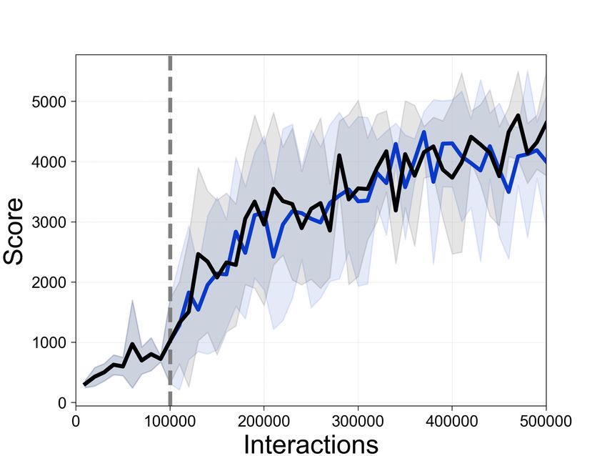
4     SEER: Stored Embeddings for Efficient Reinforcement Learning

In this section, we present SEER: Stored Embeddings for Efficient Reinforcement Learning, which
can be used in conjunction with most modern off-policy RL algorithms, such as SAC [10] and
Rainbow DQN [15]. Our main idea is to freeze lower layers during training and only update higher
layers, which eliminates the computational overhead of computing gradients and updating in lower
layers. We additionally improve the memory-efficiency of off-policy RL algorithms by storing
low-dimensional latent vectors in the replay buffer instead of high-dimensional pixel observations.
See Figure 1 and Appendix B for more details of our method.

4.1   Freezing encoder for saving computation and memory

We process high-dimensional image input with an encoder fψ to obtain zt = fψ (ot ), which is used as
input for policy πφ and Q-function Qθ as described in Section 3. In off-policy RL, we store transitions
(ot , at , ot+1 , rt ) in the replay buffer B to improve sample-efficiency by reusing experience from
the past. However, processing high-dimensional image input ot is computationally expensive. To
handle this issue, after Tf updates, we freeze the parameters of encoder ψ, and only update the policy
and Q-function. We remark that this simple technique can save computation without performance
degradation because the encoder is modeled as deep convolutional neural networks, while a shallow
MLP is used for policy and Q-function. Freezing lower layers of neural networks also has been
investigated in supervised learning based on the observation that neural networks converge to their
final representations from the bottom-up, i.e., lower layers converge very early in training [38]. For
the first time, we show the feasibility and effectiveness of this idea in pixel-based reinforcement
learning (see Figure 7a for supporting experimental results) and present solutions to its RL-specific
implementation challenges.
Moreover, in order to save memory, we consider storing (compressed) latent vectors instead of
high-dimensional image inputs. Specifically, each experience in B is replaced by the latent tran-
sition (zt , at , zt+1 , rt ), and the replay capacity is increased to C
                                                                       b (see Section 4.2 for more de-
tails). Thereafter, for each subsequent environment interaction, the latent vectors zt = fψ (ot ) and
zt+1 = fψ (ot+1 ) are computed prior to storing (zt , at , zt+1 , rt ) in B. During agent updates, the
sampled latent vectors are directly passed into the policy πφ and Q-function Qθ , bypassing the
encoder convolutional layers. Since the agent samples and trains with latent vectors after freezing,
we only store the latent vectors and avoid the need to maintain large image observations in B.

4.2   Additional techniques and details for SEER

Data augmentations. Recently, various data augmentations [41, 26, 24] have provided large gains in
the sample-efficiency of RL from pixel observations. However, SEER precludes data augmentations
because we store the latent vector instead of the raw pixel observation. We find that the absence
of data augmentations could decrease sample-efficiency in some cases, e.g., when the capacity of
B is small. To mitigate this issue, we perform K number of different data augmentations for each
input observation ot and store K distinct latent vectors {ztk = fψ (AUGk (ot ))|k = 1 · · · K}. We find
empirically that K = 4 achieves competitive performance to standard RL algorithms in most cases.
Increasing replay capacity. By storing the latent vector in the replay buffer, we can adaptively
increase the capacity (i.e., total number of transitions), which is determined by the size difference
between the input pixel observations and the latent vectors output by the encoder, with a few additional
considerations. The new capacity of the replay buffer is
                                              j             k
                                        b= C∗           P
                                        C             4N KL    ,

where C is the capacity of the original replay buffer, P is the size of the raw observation, L is
the size of the latent vector, and K is the number of data augmentations. The number of encoders
N is algorithm-specific and determines the number of distinct latent vectors encountered for each
observation during training. For Q-learning algorithms N = 1, whereas for actor-critic algorithms
N = 2 if the actor and critic each compute their own latent vectors. Some algorithms employ a target
network for updating the Q-function [32, 10], but we use the same latent vectors for the online and
target networks after freezing to avoid storing target latent vectors separately and find that tying their

                                                    4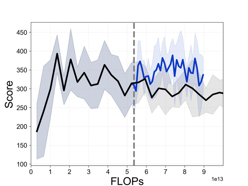
CURL CURL + SEER (ours)
Cartpole-swingup Finger-spin Reacher-easy Walker-walk Cheetah-run
1000 1000 1000 1000 600
800 800 800 800
400
Score 600 600 600 600
Score
Score
Score
Score
400 400 400 400
200
200 200 200 200
0 0 0 0 0
0 4×10¹⁴ 8×10¹⁴ 12×1014 0 2.5×10¹⁵ 5.0×10¹⁵ 0 1.5×10¹⁵ 3.0×10¹⁵ 4.5×10¹⁵ 0 2×10¹⁵ 4×10¹⁵ 6×10¹⁵ 0 1×10¹⁶ 2×10¹⁶ 3×10¹⁶
FLOPs FLOPs FLOPs FLOPs FLOPs
Figure 2: Learning curves for CURL with and without SEER, where the x-axis shows estimated
cumulative FLOPs. The dotted gray line denotes the encoder freezing time t = Tf . The solid line
and shaded regions represent the mean and standard deviation, respectively, across five runs.
Rainbow Rainbow + SEER (ours)
Alien Amidar BankHeist CrazyClimber
1400 300 40,000
300
1200 250
30,000
200 200
1000
Score
Score
Score
20,000
150
800
100
10,000
100
600
50 0 0
0 2.5×10¹³ 5.0×10¹³ 0 2.5×10¹³ 5.0×10¹³ 0 2.5×10¹³ 5.0×10¹³ 0 2×10¹³ 4×10¹³ 6×10¹³
FLOPs FLOPs FLOPs FLOPs
Krull Qbert RoadRunner Seaquest
4000 5000 15,000
600
4000
3500 500
10,000
3000
Score
Score
Score
Score
400
3000
2000
5,000 300
2500
1000 200
2000 0 0 100
0 2.5×10¹³ 5.0×10¹³ 0 2.5×10¹³ 5.0×10¹³ 0 2.5×10¹³ 5.0×10¹³ 0 2.5×10¹³ 5.0×10¹³
FLOPs FLOPs FLOPs FLOPs
Figure 3: Learning curves for Rainbow with and without SEER, where the x-axis shows estimated
cumulative FLOPs. The dotted gray line denotes the encoder freezing time t = Tf . The solid line
and shaded regions represent the mean and standard deviation, respectively, across five runs.
parameters does not degrade performance.1 The factor of 4 arises from the cost of saving floats for
latent vectors, while raw pixel observations are saved as integer pixel values. We assume the memory
required for actions and rewards is small and only consider only the memory used for observations.
5 Experimental results
We designed our experiments to answer the following questions:
• Can SEER reduce the computational overhead of various off-policy RL algorithms for both
continuous (see Figure 2) and discrete (see Figure 3) control tasks?
• Can SEER reduce the memory consumption and improve the sample-efficiency of off-policy
RL algorithms by adaptively increasing the buffer size (see Figure 4 and Figure 5)?
• Can SEER be useful for compute-efficient transfer learning (see Figure 7a)?
• Do CNN encoders of RL agents converge early in training (see Figure 8a and Figure 8b)?
5.1 Setups
Compute-efficiency. We first demonstrate the compute-efficiency of SEER on the DeepMind Control
Suite (DMControl; Tassa et al. 46) and Atari games [2] benchmarks. DMControl is commonly used
for benchmarking sample-efficiency for image-based continuous control methods. For DMControl
experiments, we consider a state-of-the-art model-free RL method, which applies contrastive learning
(CURL; Srinivas et al. 41) to SAC [10], using the image encoder architecture from SAC-AE [53].
1
We remark that the higher layers of the target network are not tied to the online network after freezing.
5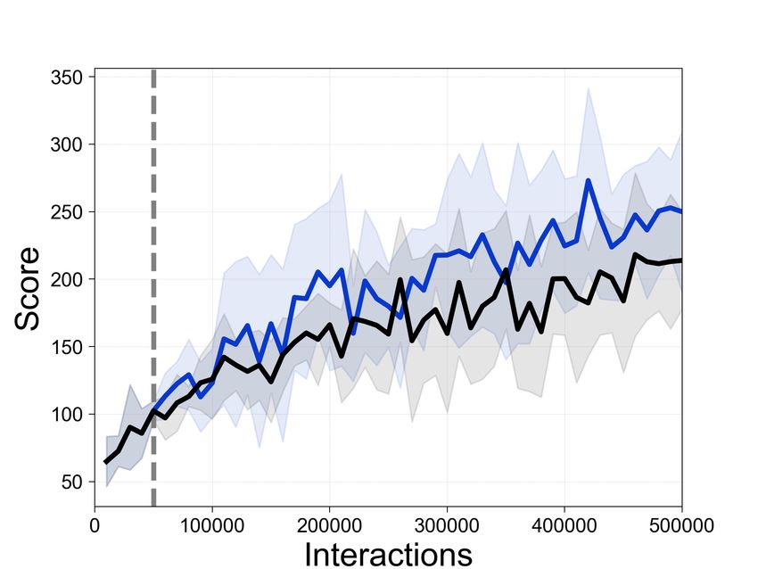
Scores at 45T FLOPs Scores at 500K environment steps (0.07GB)
Rainbow Rainbow+SEER Rainbow Rainbow+SEER
Alien 992.0 ± 152.7 1172.6 ±239.0 1038.4 ± 101.1 1134.6 ±452.9
Amidar 144.0 ± 27.4 250.5 ±47.4 121.0 ± 31.2 165.3 ±47.6
BankHeist 145.8 ± 61.2 276.6 ±98.1 161.6 ±57.7 151.8 ± 65.8
CrazyClimber 21580.0 ± 3514.6 28066.0 ±4108.5 10498.0 ± 1387.8 17620.0 ±4418.4
Krull 2799.5 ± 468.1 3277.5 ±440.5 2215.7 ± 336.9 3069.2 ±377.6
Qbert 2325.5 ± 1152.7 4123.5 ±1385.5 2430.5 ± 658.8 3231.0 ±1567.6
RoadRunner 10376.0 ± 2886.0 11794.0 ±1745.3 10612.0 ± 2059.3 13064.0 ±2489.2
Seaquest 402.8 ± 48.4 561.2 ±100.5 262.8 ± 19.1 336.8 ±45.9
Table 1: Scores on Atari games at 45T FLOPs corresponding to Figure 3 and at 500K environment
interactions in the constrained-memory setup (0.07GB) corresponding to Figure 4. The results show
the mean and standard deviation averaged five runs, and the best results are indicated in bold.
Rainbow with 3.5GB (upper bound) Rainbow with 0.07GB Rainbow + SEER with 0.07GB (ours)
Alien Amidar BankHeist CrazyClimber
250 400
1500 30,000
200 300
20,000
Score
Score
Score
1000 150 200
10,000
100 100
500
50 0 0
0 1×10⁵ 2×10⁵ 3×10⁵ 4×10⁵ 5×10⁵ 0 1×10⁵ 2×10⁵ 3×10⁵ 4×10⁵ 5×10⁵ 0 1×10⁵ 2×10⁵ 3×10⁵ 4×10⁵ 5×10⁵ 0 1×10⁵ 2×10⁵ 3×10⁵ 4×10⁵ 5×10⁵
Interactions Interactions Interactions Interactions
Krull Qbert RoadRunner Seaquest
4000 6000 15,000 600
3500 5000 12,500 500
4000 10,000
3000 400
Score
Score
Score
Score
3000 7,500
2500 300
2000 5,000
2000 1000 2,500 200
1500 0 0 100
0 1×10⁵ 2×10⁵ 3×10⁵ 4×10⁵ 5×10⁵ 0 1×10⁵ 2×10⁵ 3×10⁵ 4×10⁵ 5×10⁵ 0 1×10⁵ 2×10⁵ 3×10⁵ 4×10⁵ 5×10⁵ 0 1×10⁵ 2×10⁵ 3×10⁵ 4×10⁵ 5×10⁵
Interactions Interactions Interactions Interactions
Figure 4: Comparison of the sample-efficiency of Rainbow with and without SEER in constrained-
memory (0.07 GB) settings. The dotted gray line denotes the encoder freezing time t = Tf . The solid
line and shaded regions represent the mean and standard deviation, respectively, across five runs.
For evaluation, we compare the computational efficiency of CURL with and without SEER by
measuring floating point operations (FLOPs).2 For discrete control tasks from Atari games, we
perform similar experiments comparing the FLOPs required by Rainbow [15] with and without SEER.
For all experiments, we use the hyperparameters and architecture of data-efficient Rainbow [49].
Memory efficiency. We showcase the memory efficiency of SEER with a set of constrained-memory
experiments in DMControl. For Cartpole and Finger, the memory allocated for storing observations
is constrained to 0.03 GB, corresponding to an initial replay buffer capacity C = 1000. For Reacher
and Walker, the memory is constrained to 0.06 GB for an initial capacity of C = 2000. In this
constrained-memory setting, we compare the sample-efficiency of CURL with and without SEER.
As an upper bound, we also report the performance of CURL without memory constraints, i.e., the
replay capacity is set to the number of training steps. For Atari experiments, the baseline agent is
data-efficient Rainbow and the memory allocation is 0.07 GB, corresponding to initial replay capacity
C = 10000. The other hyperparameters are the same as those in the compute-efficiency experiments.
The encoder architecture used for our experiments with CURL is used in Yarats et al. [53]. It consists
of four convolutional layers with 3 x 3 kernels and 32 channels, with the ReLU activation applied
after each conv layer. The architecture used for our Rainbow experiments is from van Hasselt et al.
[49], consisting of a convolutional layer with 32 channels followed by a convolutional layer with
64 channels, both with 5 x 5 kernels and followed by a ReLU activation. For SEER, we freeze the
first fully-connected layer in CURL experiments and the last convolutional layer of the encoder in
Rainbow experiments. We present the best results across various values of the encoder freezing time
Tf . See Appendices H and I for more hyperparameters and Appendix A for source code.
2
We explain our procedure for counting the number of FLOPs in Appendix C.
6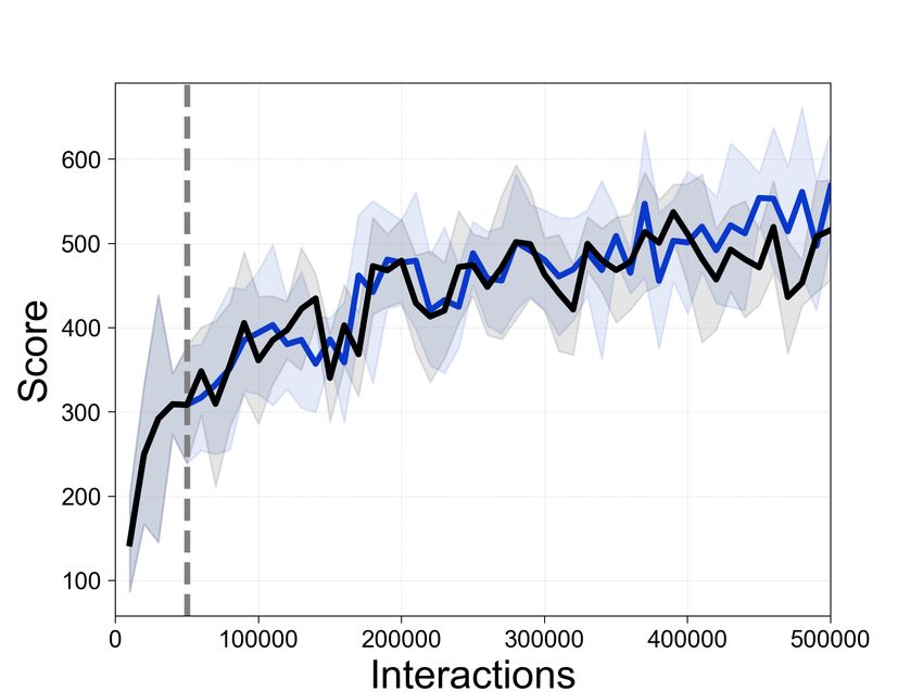
1000                                                                       1000                                                                               1000

                     800                                                                        800                                                                                800

                     600                                                                        600                                                                                600

                                                                                       Score
            Score

                                                                                                                                                                          Score
                     400                                                                        400                                                                                400

                     200                                                                        200                      CURL with 9GB (upper bound)                               200
                                       CURL with 1.8GB (upper bound)                                                                                                                                   CURL with 4.5GB (upper bound)
                                       CURL with 0.03GB                                                                  CURL with 0.03GB                                                              CURL with 0.06GB
                                       CURL + SEER with 0.03GB                                                           CURL + SEER with 0.03GB                                                       CURL + SEER with 0.06GB
                       0                                                                          0                                                                                  0
                           0   1×10⁵       2×10⁵               3×10⁵      4×10⁵                       0          1×10⁵         2×10⁵              3×10⁵           4×10⁵                  0     1×10⁵   2×10⁵    3×10⁵    4×10⁵    5×10⁵
                                        Interactions                                                                        Interactions                                                                Interactions

                     (a) Cartpole-swingup                                                                 (b) Finger-spin                                                                    (c) Reacher-easy

                                                    1000                                                                                    600

                                                     800

                                                                                                                                            400
                                            Score    600

                                                                                                                                    Score
                                                     400
                                                                                                                                            200

                                                     200                          CURL with 9GB (upper bound)                                                        CURL with 9GB (upper bound)
                                                                                  CURL with 0.06GB                                                                   CURL with 0.03GB
                                                                                  CURL + SEER with 0.06GB                                                            CURL + SEER with 0.03GB
                                                       0                                                                                      0
                                                                          5        5              5              5          5                                 5
                                                           0       1×10       2×10     3×10               4×10       5×10                         0    1×10       2×10⁵ 3×10⁵ 4×10⁵ 5×10⁵ 6×10⁵
                                                                               Interactions                                                                           Interactions

                                                               (d) Walker-walk                                                                        (e) Cheetah-run
Figure 5: Comparison of the sample-efficiency of CURL with and without SEER in constrained-
memory settings. The dotted gray line denotes the encoder freezing time t = Tf . The solid line and
shaded regions represent the mean and standard deviation, respectively, across five runs.

5.2   Improving compute- and memory-efficiency

Experimental results in DMControl and Atari showcasing the computational efficiency of SEER
are provided in Figures 2 and Figure 3. CURL and Rainbow both achieve higher performance
within significantly fewer FLOPs when combined with SEER in DMControl and Atari, respectively.
Additionally, Table 1 compares the performance of Rainbow with and without SEER at 45T (4.5e13)
FLOPs. In particular, the average returns are improved from 145.8 to 276.6 compared to baseline
Rainbow in BankHeist and from 2325.5 to 4123.5 in Qbert. We remark that SEER achieves better
computational efficiency while maintaining the agent’s final performance and comparable sample-
efficiency (see Appendix F for corresponding figures).
Experimental results in Atari and DMControl showcasing the sample-efficiency of SEER in the
constrained-memory setup are provided in Figure 4 and Figure 5. CURL and Rainbow achieve
higher final performance and better sample-efficiency when combined with SEER in DMControl and
Atari, respectively. Additionally, Table 1 compares the performance of unbounded memory Rainbow
and constrained-memory (0.07 GB) Rainbow with and without SEER at 500K interactions. In
particular, the average returns are improved from 10498.0 to 17620.0 compared to baseline Rainbow
in CrazyClimber and from 2430.5 to 3231.0 in Qbert. Although we disentangle the computational
and memory benefits of SEER in these experiments, we also highlight the computational gain of
SEER in constrained-memory settings (effectively combining the benefits) in Appendix E.

5.3   Freezing larger convolutional encoders

We also verify the benefits of SEER using deeper
convolutional encoders, which are widely used in
a range of applications such as visual navigation
tasks and favored for their superior generalization   (a) Cartpole-swingup     (b) Walker-walk
ability. Specifically, we follow the setup described
in Section 5.1 and replace the SAC-AE architec- Figure 6: Learning curves using IMPALA archi-
ture (4 convolutional layers) with the IMPALA ar- tecture, where the x-axis shows estimated cumu-
chitecture [6] (15 convolutional layers containing lative FLOPs. The dotted gray line denotes the
residual blocks [14]). Figure 5.3 shows the compu- encoder freezing time t = Tf . The solid line and
tational efficiency of SEER in Cartpole-swingup shaded regions represent the mean and standard
and Walker-walk with the IMPALA architecture. deviation, respectively, across three runs.
CURL achieves higher performance within significantly fewer FLOPs when combined with SEER.

                                                                                                                                7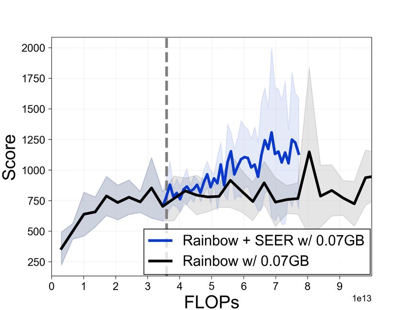
We remark that the gains due to SEER are more significant because computing and updating gradients
for large convolutional encoders is very computationally expensive.

5.4   Improving compute-efficiency in transfer settings

We demonstrate, as another application of our
method, that SEER increases compute-efficiency
in the transfer setting: utilizing the parameters
from Task A on unseen Tasks B. Specifically, we
train a CURL agent for 60K environment interac-
tions on Walker-stand; then, we only fine-tune the
policy and Q-functions on unseen tasks using net-       (a) To Walker-walk     (b) To Hopper-hop
work parameters from Walker-stand. To save com- Figure 7: Comparison of the computational
putation, during fine-tuning, we freeze the encoder efficiency of agents trained from scratch with
parameters. Figure 7a shows the computational CURL and agents trained with CURL+SEER
gain of SEER in task transfer (i.e., Walker-stand from Walker-stand pretraining. The solid line
to Walker-walk similar to Yarats et al. [53]), and and shaded regions represent the mean and stan-
domain transfer (i.e., Walker-stand to Hopper-hop) dard deviation, respectively, across three runs.
is shown in Figure 7b. Due to the generality of
CNN features, we can achieve this computational gain using a pretrained encoder. For the task transfer
setup, we provide more analysis on the number of frozen layers and freezing time hyperparameter Tf
in Appendix D.

5.5   Encoder analysis

In this subsection we present visualizations to verify that the neural networks employed in deep
reinforcement learning indeed converge from the bottom up, similar to those used in supervised
learning [38]. Figure 8a shows the spatial attention map for two Atari games and one DMControl
environment at various points during training. Similar to Laskin et al. [26] and Zagoruyko &
Komodakis [55], we compute the spatial attention map by mean-pooling the absolute values of
the activations along the channel dimension and follow with a 2-dimensional spatial softmax. The
attention map shows significant change in the first 20% of training, and remains relatively unchanged
thereafter, suggesting that the encoder converges to its final representations early in training. Figure
8b shows the SVCCA [38] score, a measure of neural network layer similarity, between a layer and
itself at time t and t + 10K. The convolutional layers of the encoder achieve high similarity scores
with themselves between time t and t + 10K, while the higher layers of the policy and Q-network
continue to change throughout training. In our DMControl environments we freeze the convolutional
layers and the first fully-connected layer of the policy and Q-network (denoted fc1). Although the
policy fc1 continues to change, the convergence of the Q-network fc1 and the encoder layers allow us
to achieve our computational and memory savings with minimal performance degradation.

6     Discussion

In this paper, we proposed a technique that reduces computation requirements for visual reinforcement
learning, which we hope serves to facilitate a shift toward more compute-efficient RL. In this section,
we highlight other techniques for reducing training time. For experimentation in computationally
intensive environments, Obando-Ceron & Castro [34] propose to use small- and medium-scale
experiments, which could reproduce the conclusions of the Rainbow DQN paper in Atari games.
For faster training time in a particular experiment, one can also lower the resolution of the input
images. In Figures 9a and 9b we show that reducing the resolution by a factor of 2, from 100 × 100 to
50 × 50 (and scaling crops appropriately) produces significant compute-efficiency gain in DeepMind
Control Suite without sacrificing performance, and emphasize that this technique can be combined
with SEER for further improved efficiency. We remark that the additional gain from SEER is larger
in more complex environments (e.g., Walker) where learning requires more steps. However, we find
that naive resolution reduction may not generally be applicable across environments and may require
domain knowledge in order to prevent excessive information loss. In Figures 9c, 9d, and 9e we
show that resolution reduction by a factor of 2, from 84 × 84 to 42 × 42, results in noticeably worse
performance in several Atari games. In contrast, SEER successfully improves compute-efficiency

                                                   8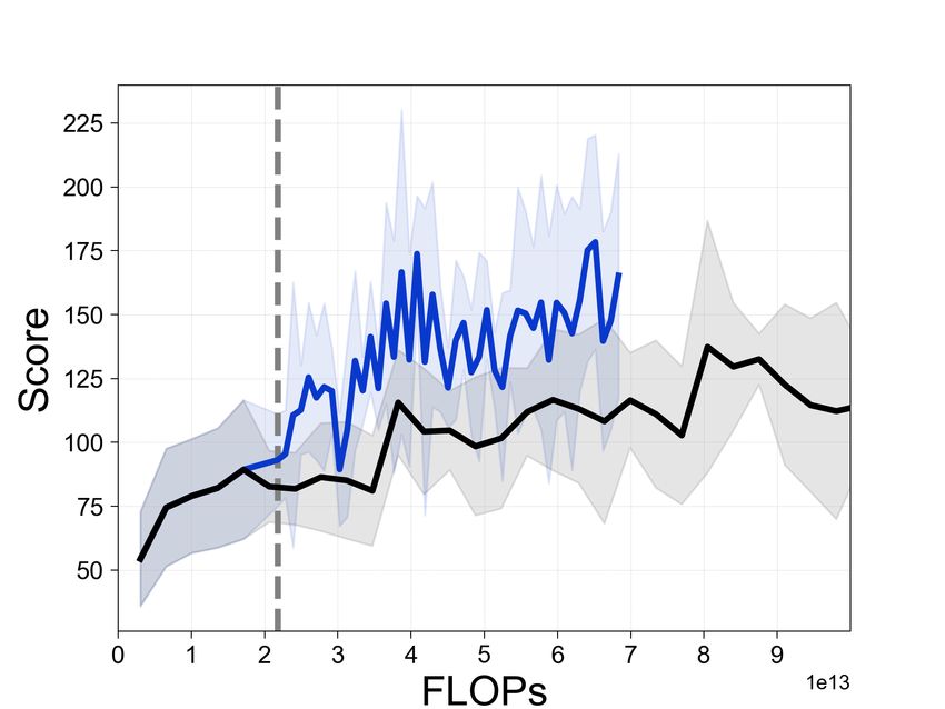
t=0

                                                                                            Time
        Alien

                                                                                                   t=100K

     Amidar

                                                                                                   t=200K

    Cartpole-
     swingup                                                                                                 conv1   conv2   conv3   conv4    fc1     fc2    fc3     fc1     fc2    fc3

                Observation   0% training   20% training   60% training 100% training                         CNN encoder                           Policy          Q-network
                                                                                                   SVCCA scale
                                                                                                                     0.0                     0.25                  0.50
                                                                                                                                                                           High similarity

                        (a) Spatial attention map                                                           (b) SVCCA similarity scores
Figure 8: Visualizations of encoder features throughout training. (a) Spatial attention map from CNN
encoders. (b) SVCCA [38] similarity scores between each layer and itself at time t and t + 10K
throughout training for Walker-walk task.

                                              (a) Cartpole-swingup                          (b) Walker-walk

                                 (c) Alien                                    (d) Amidar                                             (e) Qbert
Figure 9: Evaluation of the compute-efficiency of CURL (top) and Rainbow (bottom) with original
and reduced (by factor of 2) resolutions. The solid line and shaded regions represent the mean and
standard deviation, respectively, across five runs.

without sacrificing performance in these games (see Figure 3). Overall, SEER is highly generalizable
across visual domains, and can be easily combined with other modifications.

7    Conclusion

We presented SEER, a simple but powerful modification of off-policy RL algorithms that significantly
reduces computation and memory requirements while maintaining state-of-the-art performance. We
leveraged the intuition that CNN encoders in deep RL converge to their final representations early in
training to freeze the encoder and subsequently store latent vectors to save computation and memory.
In our experimental results, we demonstrated the compute- and memory-efficiency of SEER in
various DMControl environments and Atari games, and proposed a technique for compute-efficient
transfer learning. With SEER, we highlight the potential for improvements in compute- and memory-
efficiency in deep RL that can be made without sacrificing performance, in hopes of making deep RL
more practical and accessible in the real world.

                                                                                        9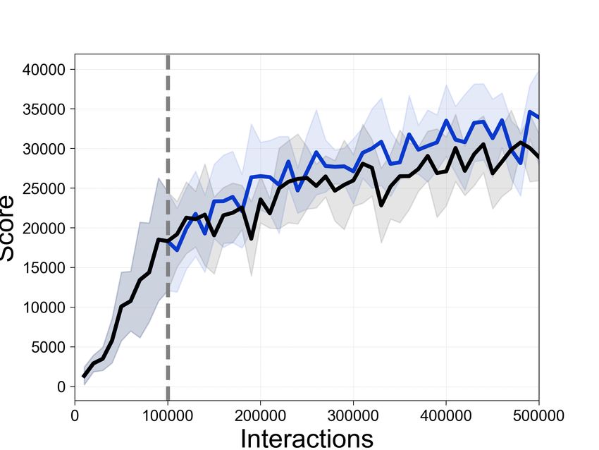
8   Acknowledgements
We would like to thank Kourosh Hakhamaneshi and Fangchen Liu for providing helpful feedback
and suggestions. We would also like to thank Denis Yarats for the IMPALA encoder architecture
implementation and Kai Arulkumaran for help with modifying the Rainbow DQN codebase.

References
 [1] Badia, Adrià Puigdomènech, Piot, Bilal, Kapturowski, Steven, Sprechmann, Pablo, Vitvitskyi,
     Alex, Guo, Daniel, and Blundell, Charles. Agent57: Outperforming the atari human benchmark.
     In International Conference on Machine Learning, 2020.
 [2] Bellemare, Marc G, Naddaf, Yavar, Veness, Joel, and Bowling, Michael. The arcade learning
     environment: An evaluation platform for general agents. Journal of Artificial Intelligence
     Research, 47:253–279, 2013.
 [3] Bellemare, Marc G, Dabney, Will, and Munos, Rémi. A distributional perspective on reinforce-
     ment learning. In International Conference on Machine Learning, 2017.
 [4] Blalock, Davis, Ortiz, Jose Javier Gonzalez, Frankle, Jonathan, and Guttag, John. What is the
     state of neural network pruning? arXiv preprint arXiv:2003.03033, 2020.
 [5] Brock, Andrew, Lim, Theodore, Ritchie, James M, and Weston, Nick. Freezeout: Accelerate
     training by progressively freezing layers. arXiv preprint arXiv:1706.04983, 2017.
 [6] Espeholt, Lasse, Soyer, Hubert, Munos, Remi, Simonyan, Karen, Mnih, Volodymir, Ward, Tom,
     Doron, Yotam, Firoiu, Vlad, Harley, Tim, Dunning, Iain, Legg, Shane, and Kavukcuoglu, Koray.
     Impala: Scalable distributed deep-rl with importance weighted actor-learner architectures, 2018.
 [7] Fang, Kuan, Toshev, Alexander, Fei-Fei, Li, and Savarese, Silvio. Scene memory transformer
     for embodied agents in long-horizon tasks. In Proceedings of the IEEE Conference on Computer
     Vision and Pattern Recognition, pp. 538–547, 2019.
 [8] Frankle, Jonathan and Carbin, Michael. The lottery ticket hypothesis: Finding sparse, trainable
     neural networks. In International Conference on Learning Representations, 2019.
 [9] Ha, David and Schmidhuber, Jürgen. World models. arXiv preprint arXiv:1803.10122, 2018.
[10] Haarnoja, Tuomas, Zhou, Aurick, Abbeel, Pieter, and Levine, Sergey. Soft actor-critic: Off-
     policy maximum entropy deep reinforcement learning with a stochastic actor. In International
     Conference on Machine Learning, 2018.
[11] Hafner, Danijar, Lillicrap, Timothy, Fischer, Ian, Villegas, Ruben, Ha, David, Lee, Honglak,
     and Davidson, James. Learning latent dynamics for planning from pixels. In International
     Conference on Machine Learning, 2019.
[12] Hafner, Danijar, Lillicrap, Timothy, Ba, Jimmy, and Norouzi, Mohammad. Dream to con-
     trol: Learning behaviors by latent imagination. In International Conference on Learning
     Representations, 2020.
[13] Han, Song, Mao, Huizi, and Dally, William J. Deep compression: Compressing deep neural net-
     works with pruning, trained quantization and huffman coding. arXiv preprint arXiv:1510.00149,
     2015.
[14] He, Kaiming, Zhang, Xiangyu, Ren, Shaoqing, and Sun, Jian. Deep residual learning for image
     recognition. In Proceedings of the IEEE conference on computer vision and pattern recognition,
     pp. 770–778, 2016.
[15] Hessel, Matteo, Modayil, Joseph, Van Hasselt, Hado, Schaul, Tom, Ostrovski, Georg, Dabney,
     Will, Horgan, Dan, Piot, Bilal, Azar, Mohammad, and Silver, David. Rainbow: Combining
     improvements in deep reinforcement learning. In AAAI Conference on Artificial Intelligence,
     2018.

                                                10
[16] Higgins, Irina, Pal, Arka, Rusu, Andrei A, Matthey, Loic, Burgess, Christopher P, Pritzel,
Alexander, Botvinick, Matthew, Blundell, Charles, and Lerchner, Alexander. Darla: Improving
zero-shot transfer in reinforcement learning. In International Conference on Machine Learning,
2017.
[17] Huang, Gao, Liu, Shichen, Van der Maaten, Laurens, and Weinberger, Kilian Q. Condensenet:
An efficient densenet using learned group convolutions. In IEEE conference on computer vision
and pattern recognition, 2018.
[18] Iandola, Forrest N, Han, Song, Moskewicz, Matthew W, Ashraf, Khalid, Dally, William J, and
Keutzer, Kurt. Squeezenet: Alexnet-level accuracy with 50x fewer parameters and< 0.5 mb
model size. arXiv preprint arXiv:1602.07360, 2016.
[19] Jaderberg, Max, Mnih, Volodymyr, Czarnecki, Wojciech Marian, Schaul, Tom, Leibo, Joel Z,
Silver, David, and Kavukcuoglu, Koray. Reinforcement learning with unsupervised auxiliary
tasks. In International Conference on Learning Representations, 2017.
[20] Jeong, Jongheon and Shin, Jinwoo. Training cnns with selective allocation of channels. In
International Conference on Machine Learning, 2019.
[21] Kaelbling, Leslie Pack, Littman, Michael L, and Cassandra, Anthony R. Planning and acting in
partially observable stochastic domains. Artificial intelligence, 101(1-2):99–134, 1998.
[22] Kaiser, Lukasz, Babaeizadeh, Mohammad, Milos, Piotr, Osinski, Blazej, Campbell, Roy H,
Czechowski, Konrad, Erhan, Dumitru, Finn, Chelsea, Kozakowski, Piotr, Levine, Sergey,
et al. Model-based reinforcement learning for atari. In International Conference on Learning
Representations, 2020.
[23] Kalashnikov, Dmitry, Irpan, Alex, Pastor, Peter, Ibarz, Julian, Herzog, Alexander, Jang, Eric,
Quillen, Deirdre, Holly, Ethan, Kalakrishnan, Mrinal, Vanhoucke, Vincent, et al. Qt-opt:
Scalable deep reinforcement learning for vision-based robotic manipulation. In Conference on
Robot Learning, 2018.
[24] Kostrikov, Ilya, Yarats, Denis, and Fergus, Rob. Image augmentation is all you need: Regulariz-
ing deep reinforcement learning from pixels. arXiv preprint arXiv:2004.13649, 2020.
[25] Lake, Brenden M, Ullman, Tomer D, Tenenbaum, Joshua B, and Gershman, Samuel J. Building
machines that learn and think like people. Behavioral and brain sciences, 40, 2017.
[26] Laskin, Michael, Lee, Kimin, Stooke, Adam, Pinto, Lerrel, Abbeel, Pieter, and Srinivas, Aravind.
Reinforcement learning with augmented data. In Advances in neural information processing
systems, 2020.
[27] LeCun, Yann, Bottou, Léon, Bengio, Yoshua, and Haffner, Patrick. Gradient-based learning
applied to document recognition. Proceedings of the IEEE, 86(11):2278–2324, 1998.
[28] Lee, Kimin, Laskin, Michael, Srinivas, Aravind, and Abbeel, Pieter. Sunrise: A simple
unified framework for ensemble learning in deep reinforcement learning. arXiv preprint
arXiv:2007.04938, 2020.
[29] Lillicrap, Timothy P, Hunt, Jonathan J, Pritzel, Alexander, Heess, Nicolas, Erez, Tom, Tassa,
Yuval, Silver, David, and Wierstra, Daan. Continuous control with deep reinforcement learning.
In International Conference on Learning Representations, 2016.
[30] Lin, Long-Ji. Self-improving reactive agents based on reinforcement learning, planning and
teaching. Machine learning, 8(3-4):293–321, 1992.
[31] Mattson, Peter, Cheng, Christine, Coleman, Cody, Diamos, Greg, Micikevicius, Paulius, Patter-
son, David, Tang, Hanlin, Wei, Gu-Yeon, Bailis, Peter, Bittorf, Victor, et al. Mlperf training
benchmark. In Conference on Machine Learning and Systems, 2020.
[32] Mnih, Volodymyr, Kavukcuoglu, Koray, Silver, David, Rusu, Andrei A, Veness, Joel, Bellemare,
Marc G, Graves, Alex, Riedmiller, Martin, Fidjeland, Andreas K, Ostrovski, Georg, et al.
Human-level control through deep reinforcement learning. Nature, 518(7540):529, 2015.
11[33] Morcos, Ari, Raghu, Maithra, and Bengio, Samy. Insights on representational similarity in
neural networks with canonical correlation. In Advances in Neural Information Processing
Systems, 2018.
[34] Obando-Ceron, Johan S and Castro, Pablo Samuel. Revisiting rainbow: Promoting more
insightful and inclusive deep reinforcement learning research. arXiv preprint arXiv:2011.14826,
2020.
[35] Oord, Aaron van den, Li, Yazhe, and Vinyals, Oriol. Representation learning with contrastive
predictive coding. arXiv preprint arXiv:1807.03748, 2018.
[36] Osband, Ian, Blundell, Charles, Pritzel, Alexander, and Van Roy, Benjamin. Deep exploration
via bootstrapped dqn. In Advances in neural information processing systems, 2016.
[37] Pellegrini, Lorenzo, Graffieti, Gabrile, Lomonaco, Vincenzo, and Maltoni, Davide. Latent
replay for real-time continual learning. arXiv preprint arXiv:1912.01100, 2019.
[38] Raghu, Maithra, Gilmer, Justin, Yosinski, Jason, and Sohl-Dickstein, Jascha. Svcca: Singular
vector canonical correlation analysis for deep understanding and improvement. In Advances in
neural information processing systems, 2017.
[39] Schrittwieser, Julian, Antonoglou, Ioannis, Hubert, Thomas, Simonyan, Karen, Sifre, Lau-
rent, Schmitt, Simon, Guez, Arthur, Lockhart, Edward, Hassabis, Demis, Graepel, Thore,
et al. Mastering atari, go, chess and shogi by planning with a learned model. arXiv preprint
arXiv:1911.08265, 2019.
[40] Schulman, John, Chen, Xi, and Abbeel, Pieter. Equivalence between policy gradients and soft
q-learning. arXiv preprint arXiv:1704.06440, 2017.
[41] Srinivas, Aravind, Laskin, Michael, and Abbeel, Pieter. Curl: Contrastive unsupervised
representations for reinforcement learning. In International Conference on Machine Learning,
2020.
[42] Stooke, Adam, Lee, Kimin, Abbeel, Pieter, and Laskin, Michael. Decoupling representation
learning from reinforcement learning, 2020.
[43] Sun, Zhiqing, Yu, Hongkun, Song, Xiaodan, Liu, Renjie, Yang, Yiming, and Zhou, Denny.
Mobilebert: a compact task-agnostic bert for resource-limited devices. In Annual Meeting of
the Association for Computational Linguistics, 2020.
[44] Sutton, Richard S. Dyna, an integrated architecture for learning, planning, and reacting. ACM
Sigart Bulletin, 2(4):160–163, 1991.
[45] Sutton, Richard S and Barto, Andrew G. Reinforcement learning: An introduction. MIT Press,
2018.
[46] Tassa, Yuval, Doron, Yotam, Muldal, Alistair, Erez, Tom, Li, Yazhe, Casas, Diego de Las,
Budden, David, Abdolmaleki, Abbas, Merel, Josh, Lefrancq, Andrew, et al. Deepmind control
suite. arXiv preprint arXiv:1801.00690, 2018.
[47] Tay, Yi, Zhang, Aston, Tuan, Luu Anh, Rao, Jinfeng, Zhang, Shuai, Wang, Shuohang, Fu,
Jie, and Hui, Siu Cheung. Lightweight and efficient neural natural language processing with
quaternion networks. In Annual Meeting of the Association for Computational Linguistics,
2019.
[48] Van Hasselt, Hado, Guez, Arthur, and Silver, David. Deep reinforcement learning with double
q-learning. In AAAI Conference on Artificial Intelligence, 2016.
[49] van Hasselt, Hado P, Hessel, Matteo, and Aslanides, John. When to use parametric models in
reinforcement learning? In Advances in Neural Information Processing Systems, pp. 14322–
14333, 2019.
[50] Vaswani, Ashish, Shazeer, Noam, Parmar, Niki, Uszkoreit, Jakob, Jones, Llion, Gomez, Aidan N,
Kaiser, Łukasz, and Polosukhin, Illia. Attention is all you need. In Advances in neural
information processing systems, 2017.
12[51] Vinyals, Oriol, Babuschkin, Igor, Czarnecki, Wojciech M, Mathieu, Michaël, Dudzik, Andrew,
Chung, Junyoung, Choi, David H, Powell, Richard, Ewalds, Timo, Georgiev, Petko, et al.
Grandmaster level in starcraft ii using multi-agent reinforcement learning. Nature, 575(7782):
350–354, 2019.
[52] Watkins, Christopher JCH and Dayan, Peter. Q-learning. Machine learning, 8(3-4):279–292,
1992.
[53] Yarats, Denis, Zhang, Amy, Kostrikov, Ilya, Amos, Brandon, Pineau, Joelle, and Fergus, Rob.
Improving sample efficiency in model-free reinforcement learning from images. arXiv preprint
arXiv:1910.01741, 2019.
[54] Yosinski, Jason, Clune, Jeff, Bengio, Yoshua, and Lipson, Hod. How transferable are features
in deep neural networks? In Advances in neural information processing systems, 2014.
[55] Zagoruyko, Sergey and Komodakis, Nikos. Paying more attention to attention: Improving the
performance of convolutional neural networks via attention transfer. In International Conference
on Learning Representations, 2017.
[56] Ziebart, Brian D. Modeling purposeful adaptive behavior with the principle of maximum causal
entropy. 2010.
13Appendix
A Source Code
We provide source code in https://github.com/lili-chen/SEER.
B Algorithm
We detail the specifics of modifying off-policy RL methods with SEER in Algorithm 1. For concrete-
ness, we describe SEER combined with deep Q-learning methods.
Algorithm 1 Stored Embeddings for Efficient Reinforcement Learning (DQN Base Agent)
1: Initialize replay buffer B with capacity C
2: Initialize action-value network Q with parameters θ and encoder f with parameters ψ
3: for each timestep t do
4: Select action: at ← argmaxa Qθ (fψ (ot ), a)
5: Collect observation ot+1 and reward rt from the environment by taking action at
6: if t ≤ Tf then
7: Store transition (ot , at , ot+1 , rt ) in replay buffer B
8: else
9: Compute latent states zt , zt+1 ← fψ (ot ), fψ (ot+1 )
10: Store transition (zt , at , zt+1 , rt ) in replay buffer B
11: end if
12: // R EPLACE PIXEL - BASED TRANSITIONS WITH LATENT TRAJECTORIES
13: if t = Tf then
min(T ,c) min(T ,c)
14: Compute latent states {(zt , zt+1 )}t=1 f ← {(fψ (ot ), fψ (ot+1 ))}t=1 f
min(T ,c) min(T ,c)
15: Replace {(ot , at , ot+1 , rt )}t=1 f with latent transitions {(zt , at , zt+1 , rt )}t=1 f
16: Increase the capacity of B to C b
17: end if
18: // U PDATE PARAMETERS OF Q- NETWORK WITH SAMPLED IMAGES OR LATENTS
19: for each gradient step do
20: if t < Tf then
21: Sample random minibatch {(oj , aj , oj+1 , rj )}bj=1 ∼ B
22: Calculate target yj = rj + γ maxa0 Qθ̄ (fψ̄ (oj+1 ), a0 )
23: Perform a gradient step on LDQN (θ, ψ)
24: else
25: Sample random minibatch {(zj , aj , zj+1 , rj )}bj=1 ∼ B
26: Calculate target yj = rj + γ maxa0 Qθ̄ (zj+1 , a0 )
27: Perform a gradient step on LDQN (θ)
28: end if
29: end for
30: end for
C Calculation of Floating Point Operations
We consider each backward pass to require twice as many FLOPs as a forward pass. 3 Each weight
requires one multiply-add operation in the forward pass. In the backward pass, it requires two
multiply-add operations: at layer i, the gradient of the loss with respect to the weight at layer i and
with respect to the output of layer (i − 1) need to be computed. The latter computation is necessary
for subsequent gradient calculations for weights at layer (i − 1).
3
This method for FLOP calculation is used in https://openai.com/blog/ai-and-compute/.
14We use functions from Huang et al. [17] and Jeong & Shin [20] to obtain the number of operations
per forward pass for all layers in the encoder (denoted E) and number of operations per forward pass
for all MLP layers (denoted M ).
We denote the number of forward passes per training update F , the number of backward passes per
training update B, and the batch size b. We assume the number of updates per timestep is 1. Then,
the number of FLOPs per iteration before freezing at time t = Tf is:
bF (E + M ) + 2bB(E + M ) + (E + M ),
where the last term is for the single forward pass required to compute the policy action. For the
baseline, FLOPs are computed using this formula throughout training.
SEER reduces computational overhead by eliminating most of the encoder forward and backward
passes. The number of FLOPs per iteration after freezing is:
bF M + 2bBM + (E + M ) + EKN,
where K is the number of data augmentations and N is the number of networks as described in
Section 4.2. The forward and backward passes of the encoder for training updates are removed, with
the exception of the forward pass for computing the policy action and the EKN term at the end that
arises from calculating latent vectors for the current observation.
At freezing time t = Tf , we need to compute latent vectors for each transition in the replay buffer.
This introduces a one-time cost of (EKN min(Tf , C)) FLOPs, since the number of transitions in
the replay buffer is min(Tf , C), where C is the initial replay capacity.
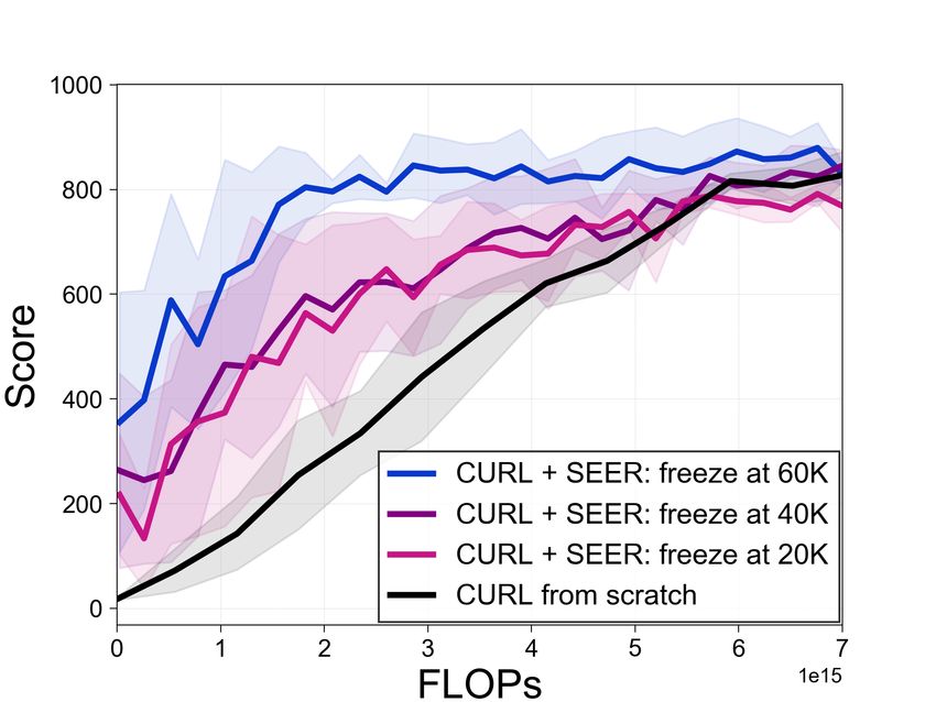
D Transfer Setting Analysis
In Figure 7a we show the computational efficiency of SEER on Walker-walk with Walker-stand
pretrained for 60K steps, with four convolutional layers frozen. We provide analysis for the number
of layers frozen and number of environment interactions before freezing Tf in Figure 10. We find that
freezing more layers allows for more computational gain, since we can avoid computing gradients for
the frozen layers without sacrificing performance. Longer pretraining in the source task improves
compute-efficiency in the target task; however, early convergence of encoder parameters enables the
agent to learn a good policy even with only 20K interactions before transfer.
We remark that Yosinski et al. [54] examine the generality of features learned by neural networks
and the feasibility of transferring parameters between similar image classification tasks. Yarats et al.
[53] show that transferring encoder parameters pretrained from Walker-walk to Walker-stand and
Walker-run can improve the performance and sample-efficiency of a SAC agent. For the first time,
we show that encoder parameters trained on simple tasks can be useful for compute-efficient training
in complex tasks and new domains.
E Compute-Efficiency in Constrained-Memory Settings
In our main experiments, we isolate the two major contributions of our method, reduced computational
overhead and improved sample-efficiency in constrained-memory settings. In Figure 11 we show
that these benefits can also be combined for significant computational gain in constrained-memory
settings.
F Sample-Efficiency Plots
In section 5.2 we show the compute-efficiency of our method in DMControl and Atari environments.
We show in Figure 12 that our sample-efficiency is very close to that of baseline CURL [41], with
only slight degradation in Cartpole-swingup and Walker-walk. In Atari games (Figure 13), we match
the sample-efficiency of baseline Rainbow [15] very closely, with no degradation.
15(a) Number of frozen layers. (b) Freezing time hyperparameter Tf .
Figure 10: (a) Analysis on the number of frozen convolutional layers in Walker-walk training from
Walker-stand pretrained for 60K steps. (b) Analysis on the number of environment steps Walker-stand
agent is pretrained prior to Walker-walk transfer, where the first four convolutional layers are frozen.
(a) Alien (b) Amidar (c) BankHeist (d) CrazyClimber
(e) Krull (f) Qbert (g) RoadRunner (h) Seaquest
Figure 11: Comparison of Rainbow in constrained-memory settings with and without SEER, where
the x-axis shows estimated cumulative FLOPs, corresponding to Figure 4. The dotted gray line
denotes the encoder freezing time t = Tf . The solid line and shaded regions represent the mean and
standard deviation, respectively, across five runs.
G General Implementation Details
SEER can be applied to any convolutional encoder which compresses the input observation into a
latent vector with smaller dimension than the observation. We generally freeze all the convolutional
layers and possibly the first fully-connected layer. In our main experiments, we chose to freeze the
first fully-connected layer for DM Control experiments and the last convolutional layer for Atari
experiments. We made this choice in order to simultaneously save computation and memory; for
those architectures, if we freeze an earlier layer, we save less computation, and the latent vectors
(convolutional features) are too large for our method to save memory. In DM Control experiments,
the latent dimension of the first fully-connected layer is 50, which allows a roughly 12X memory
gain. In Atari experiments, the latent dimension of the last convolutional layer is 576, which allows a
roughly 3X memory gain.
H DMControl Implementation details
We use the network architecture in https://github.com/MishaLaskin/curl for our CURL [41]
implementation. We show a full list of hyperparameters in Table 2.
16(a) Cartpole-swingup (b) Finger-spin (c) Reacher-easy
(d) Cheetah-run (e) Walker-walk
Figure 12: Comparison of the sample-efficiency of CURL with and without SEER, corresponding to
Figure 2. The dotted gray line denotes the encoder freezing time t = Tf . The solid line and shaded
regions represent the mean and standard deviation, respectively, across five runs.
(a) Alien (b) Amidar (c) BankHeist (d) CrazyClimber
(e) Krull (f) Qbert (g) RoadRunner (h) Seaquest
Figure 13: Comparison of the sample-efficiency of Rainbow with and without SEER, corresponding
to Figure 3. The dotted gray line denotes the encoder freezing time t = Tf . The solid line and shaded
regions represent the mean and standard deviation, respectively, across five runs.
I Atari Implementation details
We use the network architecture in https://github.com/Kaixhin/Rainbow for our Rainbow
[15] implementation and the data-efficient Rainbow [49] encoder architecture and hyperparameters.
We show a full list of hyperparameters in Table 3.
17Table 2: Hyperparameters used for DMControl experiments. Most hyperparameter values are
unchanged across environments with the exception of initial replay buffer size, action repeat, and
learning rate.
Hyperparameter Value
Augmentation Crop
Observation rendering (100, 100)
Observation down/upsampling (84, 84)
Replay buffer size in Figure 2 Number of training steps
Initial replay buffer size in Figure 5 1000 cartpole, swingup; cheetah, run; finger, spin
2000 reacher, easy; walker, walk
Number of updates per training step 1
Initial steps 1000
Stacked frames 3
Action repeat 2 finger, spin; walker, walk
4 cheetah, run; reacher, easy
8 cartpole, swingup
Hidden units (MLP) 1024
Evaluation episodes 10
Evaluation frequency 2500 cartpole, swingup
10000 cheetah, run; finger, spin; reacher, easy; walker, walk
Optimizer Adam
(β1 , β2 ) → (fψ , πφ , Qθ ) (.9, .999)
(β1 , β2 ) → (α) (.5, .999)
Learning rate (fψ , πφ , Qθ ) 2e − 4 cheetah, run
1e − 3 cartpole, swingup; finger, spin; reacher, easy; walker, walk
Learning rate (α) 1e − 4
Batch Size 512 cheetah, run
128 cartpole, swingup; finger, spin; reacher, easy; walker, walk
Q function EMA τ 0.01
Critic target update freq 2
Convolutional layers 4
Number of filters 32
Non-linearity ReLU
Encoder EMA τ 0.05
Latent dimension 50
Discount γ .99
Initial temperature 0.1
Freezing time Tf in Figure 2 10000 cartpole, swingup
50000 finger, spin; reacher, easy
60000 walker, walk
80000 cheetah, run
Freezing time Tf in Figure 5 10000 cartpole, swingup
50000 finger, spin
30000 reacher, easy
80000 cheetah, run; walker, walk
18Table 3: Hyperparameters used for Atari experiments. All hyperparameter values are unchanged
across environments with the exception of encoder freezing time.
Hyperparameter Value
Augmentation None
Observation rendering (84, 84)
Replay buffer size in Figure 3 Number of training steps
Initial replay buffer size in Figure 4 10000
Number of updates per training step 1
Initial steps 1600
Stacked frames 4
Action repeat 1
Hidden units (MLP) 256
Evaluation episodes 10
Evaluation frequency 10000
Optimizer Adam
(β1 , β2 ) → (fψ , Qθ ) (.9, .999)
Learning rate (fψ , Qθ ) 1e − 3
Learning rate (α) 0.0001
Batch Size 32
Multi-step returns length 20
Critic target update freq 2000
Convolutional layers 2
Number of filters 32, 64
Non-linearity ReLU
Discount γ .99
Freezing time Tf in Figure 3 50000 Alien; Amidar; BankHeist; Krull; RoadRunner; Seaquest
100000 CrazyClimber; Qbert
Freezing time Tf in Figure 4 50000 Amidar; BankHeist; Krull; RoadRunner
100000 Alien; CrazyClimber; Qbert
150000 Seaquest
19You can also read


