Implementation of arbitrary polyhedral elements for automatic dynamic analyses of three dimensional structures
←
→
Page content transcription
If your browser does not render page correctly, please read the page content below
www.nature.com/scientificreports
OPEN Implementation of arbitrary
polyhedral elements
for automatic dynamic analyses
of three‑dimensional structures
Lei Zhou1,2, Jianbo Li1,2* & Gao Lin1,2
The transition from the geometry to the mesh can be rather difficult, manual and time-consuming,
especially for the large scale complex structures. The procedure of mesh generation needs massive
human intervention making the automatic engineering analyses of structures from CAD geometry
models hardly possible. This paper focuses on implementing a polyhedron element with arbitrary
convex topology based on the Scaled Boundary Finite Element Method (SBFEM) in ABAQUS on
the strength of the interface of UEL (the subroutine to define a general user-defined element) for
automatic dynamic analyses of three-dimensional structures. This implementation empowers
ABAQUS to analyze any model with arbitrary polyhedron elements. When the geometry of a structure
is obtained from CAD, the dynamic analyses can be launched seamlessly and automatically. Cases of
a cantilever subjected to a dynamic harmonic excitation with the traditional hexahedron element and
this polyhedron element are compared to verify the accuracy of the UEL. Taking a practical example of
the Soil-Structure Interaction analysis of a Nuclear Power Plant, the applicability and performance of
this implementation are tested. The results of the two examples confirm that this polyhedron element
based on SBFEM can be more accurate using much less degrees of freedom and its implementation in
ABAQUS is robust and compatible.
As the development of the Computer Aided Design (CAD) and Computer Aided Engineering (CAE) tools in
the industry, the design, safety assessment, health monitoring of some important modern infrastructures tend to
need more and more refined and sophisticated geometry models and mesh models. Nevertheless, there is a gap
between the CAD and the CAE holding a barrier between the geometry model for design and the mesh model
for engineering analysis. Because except for some rarely used meshless methods, it is a difficult, manual and
time-consuming process to generate a fine mesh from a complex geometry. During the manual mesh generation,
the balance of accuracy and efficiency should be examined, especially for dynamic analysis in the time domain. A
basic requirement is to assign heterogeneous distributed grid densities for the different location of the geometry
model to balance the calculation accuracy and efficiency, which are case-sensitive, completely experimental and
can be rather tedious. The automatic mesh generation technique with polyhedron elements can break this barrier
due to the flexible topology that makes them highly adaptable to the complex shape and smooth transition of
mesh density, which is the foundation of the automatic engineering analysis.
Since the arising of numerical methods for the Partial Differential Equation (PDE), the mesh generation has
become a primary procedure for these methods that need spatial discretization like the Finite Element Method
(FEM) and the Finite Difference Method (FDM). From a geometrical point of view, a mesh is the approximate
shape representation of the domains or the media (or can be collectively referred to as configurations) of the
original physical problem, which consists of many non-overlapping continuous small domains called elements.
These elements have certain topology defined by geometric feature points such as vertices called nodes, where
the degrees of freedom are defined on. Except that a numerical analysis cannot be carried on without a mesh,
the quality, size and type of the mesh have a great influence on the reliability of the results as well.
For the last four decades, lots of mesh generation technologies have been developed from two-dimension
(2D) domain to three-dimension (3D) domain on the strength of the computer graphics. During the 1950s, mesh
generation techniques based on coordinate transformations firstly came up, such as the conformal m apping1,2
1
State Key Laboratory of Coastal and Offshore Engineering, Dalian University of Technology, 2 Linggong Road,
Dalian 116024, China. 2Institute of Earthquake Engineering, Faculty of Infrastructure Engineering, Dalian
University of Technology, 2 Linggong Road, Dalian 116024, China. *email: jianboli@dlut.edu.cn
Scientific Reports | (2022) 12:4156 | https://doi.org/10.1038/s41598-022-07996-6 1
Vol.:(0123456789)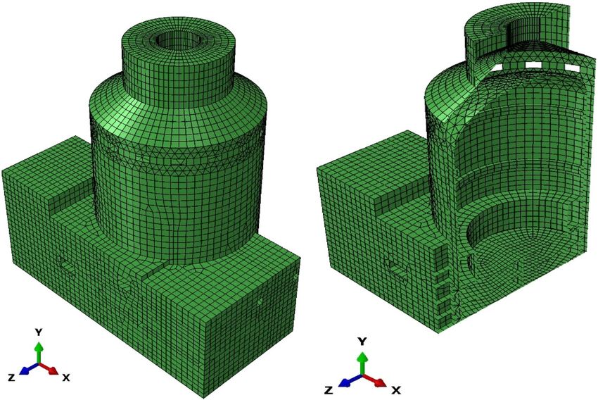
www.nature.com/scientificreports/
technique. This technique was extended to simple 3D configurations by South et al.3 and Baker4. Although the
methods above can generate structured hexahedral or quadrilateral meshes with high quality, the process of these
methods requires lots of time, manual guidance and very specific geometry. In the 1980s, triangulation methods
emerged generating unstructured triangular meshes for 2D configurations or tetrahedral meshes for 3D configu-
rations. After the generation of a triangulation mesh, an unstructured hexahedral mesh can be obtained by the
domain partition5–8. Unstructured meshes can always be created by triangulation methods for any intricate geom-
etry automatically and efficiently. But these kinds of meshes have low accuracy and additional artificial stiffness,
especially the first order ones. On the other hand, for a same domain the degrees of freedom of a triangulation
mesh are much more than those of a hexahedral or quadrilateral mesh. If the mesh requirement of conforming
the boundary is omitted, the Cartesian methods can automatically generate octree meshes that contain particular
polyhedron elements without creating surface meshes. But the mesh created by this method has a poor accuracy
on boundary vicinity leading to an inaccurate boundary condition. At the moment, for complex geometries only
the polyhedron mesh generation technique can be fully automatic with few human interventions.
Polyhedron meshes such as octree meshes have been widely used in fluid mechanics exhibiting many topo-
logical properties that make them highly and automatically adaptable to the complex shape and smooth transi-
tion of mesh density9,10. Nevertheless, the application of polyhedron elements for continuum mechanics is few
because the topology of a polyhedron is inconstant. Hence it is impossible to construct analytic shape functions
for arbitrary polyhedron elements with varying topologies. Some kind of interpolation schemes must be applied.
Two kinds of interpolation schemes were developed. The first one was based on natural neighbor interpola-
tions proposed by Sibson11,12. Traversoni13 and Sambridge et al.14 introduced Sibson interpolations modified by
Watson15 to the Galerkin-type natural neighbor, which was extended to continuum by Sukumar et al.16,17. Belikov
et al. raised the Laplacian and non-Sibson interpolants18,19 and the polygonal finite element interpolants20,21. The
other one was built on generalized barycentric coordinates, which was brought up by W achspress22. This kind of
interpolants was further developed by W arren23,24, Meyer et al.25, Floater et al.26,27, Lipman28, and Warren et al.29.
However, the interpolation scheme generally needs considerable calculation to get adequate accuracy.
Another approach to constructing polyhedral elements is to utilize SBFEM. In mid-1990s, SBFEM also known
as the consistent infinitesimal finite-element-cell method was bought up by Wolf and Song as an extension to
FEM to simulate the wave propagation in the unbounded d omain30–33. As a similarity-based semi-analytical
numerical approach for PDE, SBFEM has many advantages over the traditional FEM and Boundary Element
Method (BEM) exhibiting high accuracy and flexibility34,35. SBFEM just needs boundary discretization reducing
the problem spatial dimension by one with no need for a fundamental solution and the solution along the radial
direction is in a precise closed-form. For the unbounded media, SBFEM can perfectly satisfy the boundary condi-
tion of the radiation damping. The unit-impulse response matrix in the time domain and the dynamic-stiffness
matrix in the frequency domain of the unbounded media can be directly obtained, which is equivalent to a time
and space coupling artificial non-reflecting boundary36. For the bounded media, the SBFEM is derived in a wedge
media. The wedge media can be assembled into an arbitrary convex polyhedron (3D) or polygon (2D) super
element revolving around the similarity center. If this assembly is not occlusive and the crack tip is positioned
in the similarity center, the singularity of the field function can be directly described by the analytical solution
along the radical crack surface. This superiority of mesh adaptability can be combined with the automatic mesh
generation technique based on polyhedron elements.
The first try was a SBFEM formulation for arbitrary polyhedral elements and a simple method to generate
polyhedral meshes based on octree presented by Talebi et al.37. To automatically generate an octree polyhedral
mesh from the Standard Tessellation Language (STL) widely used in the 3D printing and Computer Aided
Design (CAD), Liu et al.38 came up with a two-steps method. The first step is to generate an octree mesh within
the domain enclosed by the surface defined in the STL. The second step is to cut the polyhedral elements with
the surface. After the refinement of the second step, the poor boundary accuracy of the octree mesh is improved.
Furthermore, Zhang et al.39 applied the SBFEM polyhedral elements to the non-matching meshes by adding
nodes to the elements adjacent to the interface. By now, there is a slight limitation when using SBFEM polyhe-
dral elements. Since the boundary is discretized by FEM elements, the facets of a polyhedral element must be
a triangle or quadrilateral, which may lead to a facet division process. To resolve this limitation of SBFEM, Ooi
et al.40 derived a dual SBFEM formulation over arbitrary faceted star convex polyhedron. On the other hand,
Zou et al.41 brought up a FEM polyhedral element formulation with shape functions derived from SBFEM cir-
cumventing this limitation as well. The automatic polyhedral element based on SBFEM was applied to dynamic
nonlinear analysis of hydraulic e ngineering42, concrete fracture m
odelling43, damage modelling44,45, Soil-Structure
46
Interaction (SSI) analysis of N PP , etc. These applications of SBFEM polyhedral meshes were mostly imple-
mented by self-developed programs. Few of them integrate the SBFEM into the universal FEM software such
as ABAQUS43,47. And these integrations is suitable for traditional FEM elements with fixed topologies only. The
integration of SBFEM and the universal FEM software can promote each other. Implementation of arbitrary
polyhedral elements in ABAQUS is still in need.
In this paper, arbitrary polyhedron elements based on SBFEM for three dimensional continuum is developed
and implemented in ABAQUS facilitating automatic dynamic analyses of structures. The governing equation of
the bounded 3D elastic continuum in a polyhedron domain is derived from the SBFEM in “SBFEM governing
equation for the elastic continuum” section. The FEM-coupled characteristic matrix of a polyhedron element can
be obtained from the solution of the governing equation. The topology feature and corresponding data structure
of a polyhedron is analyzed in “Topology and data structure of an arbitrary polyhedron element” section. The
user element subroutine of UEL is developed associated with the Hilber-Hughes-Taylor (HHT) implicit time
integration scheme in “Implementation in ABAQUS’ section. In “Numerical application” section, there are two
examples for the UEL. A cantilever subjected to a harmonic excitation with the traditional hexahedron element
and the SBFEM-based polyhedron element are compared to confirm the accuracy of the UEL. Then taking a
Scientific Reports | (2022) 12:4156 | https://doi.org/10.1038/s41598-022-07996-6 2
Vol:.(1234567890)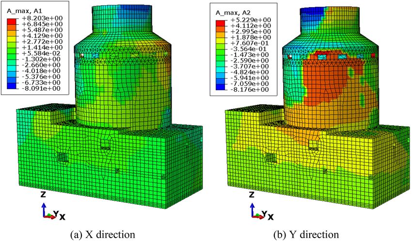
www.nature.com/scientificreports/
(a) S-element in bounded domain (b) S-element in unbounded domain
Figure 1. Spatial discretization of SBFEM for (a) S-element in bounded domain, (b) S-element in unbounded
domain.
Figure 2. Bounded domain divided by three S-elements.
practical example of the soil-structure dynamic interaction analysis of a nuclear power plant, the applicability
and performance of this implementation of polyhedron elements is tested.
SBFEM governing equation for the elastic continuum
SBFEM is a numerical method for solving PDE. The PDE is transformed into ordinary differential equations after
specific spatial discretization, which is different from FEM, BEM, etc. SBFEM needs boundary discretization
only decreasing the spatial dimension by 1 and remains analytical in the radial direction without the need of a
foundation solution. The derivation of the SBFEM governing equation of elastic continuum is based on a wedge
area defined as W-element. The governing equations of W-elements that shared the same scaling center can be
assembled by degrees of freedom of adjacent W-elements (see Fig. 1) leading to a piece-wise boundary of the
discretized domain defined as an S-element. The choice of the scaling center location can be pretty casual. The
boundary of the discretized domain must be visible from the scaling center is the only geometry requirement that
needs to be satisfied. The bounded domain can be divided into multiple S-elements to meet the requirement of
the scaling center or to improve the poor geometry of W-elements (see Fig. 2). Apparently, the geometry of the
S-element can be rather flexible for any convex polyhedron with only triangle or quadrilateral facets.
The detailed derivation of SBFEM governing equation is well documented in many l iteratures33,48–52. For the
sake of integrity, only key equations are given below. The equations in this section are given in linear algebraic
notation for the convenience of reading and programming. The brace symbol of {·} denotes a matrix and the
bracket symbol of [·] denotes a column vector.
Scientific Reports | (2022) 12:4156 | https://doi.org/10.1038/s41598-022-07996-6 3
Vol.:(0123456789)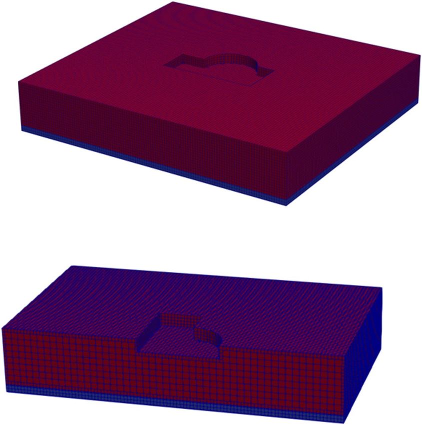
www.nature.com/scientificreports/
Partial differential equations of dynamic elastic mechanics. According to the theory of continuum
mechanics, three basic equations are derived as
[A]{σ } + f = {0}, (1)
{ε} = [L]{u}, (2)
{σ } = [D]{ε}, (3)
where [A] denotes the spatial partial derivative operator, {σ } denotes the stress vector, {ε} denotes the strain vec-
tor, f denotes the body forces that include the inertial force for the dynamic analysis. The detailed definitions
of them are
∂ ∂ ∂
∂x 0 0 ∂y 0 ∂z
∂ ∂ ∂
[A] = 0 ∂y 0 ∂x ∂z 0 , (4)
∂ ∂ ∂
0 0 ∂z 0 ∂y ∂x
σx
σy
� � �� σz
σ x, y, z =
τxy
, (5)
τ
yz
τzx
� �
� � �� fx �x, y, z � � � �� � � ��
f x, y, z = fy �x, y, z � = p x, y, z − ρ ü x, y, z . (6)
fz x, y, z
The equilibrium equations (Eq. (1)), the geometric equations (Eq. (2)) and the constitutive equations (Eq. (3))
can be combined into one set of partial differential equations of 3D dynamic elastic mechanics with the displace-
ment vector filed as the unknown variable as
� �
[L]T [D][L]{u} + p − ρ{ü} = {0},
∂
∂x 0 0
0 ∂ 0
∂y
T
0 0 ∂
∂z (7)
[L] = [A] = ∂ ∂ ,
∂y ∂x 0
∂ ∂
0 ∂z ∂y
∂ ∂
∂z 0 ∂x
T
where u x, y, z = ux x, y, z
uy x, y, z uz x, y, z denotes the displacement vector filed, [D] denotes
the material property matrix, p denotes the body forces except the d’Alembert inertial force, ρ denotes the
density, [L] denotes the spatial partial derivative operator.
The linear elastic material property matrix [D] is given by
+ 2G 0 0 0
+ 2G 0 0 0
+ 2G 0 0 0
[D] = 0 0 0 G 0 0 ,
0 0 0 0 G 0 (8)
0 0 0 0 0 G
Eν E
= , G= ,
(1 + ν)(1 − 2ν) 2(1 + ν)
where denotes the Lame parameter, E denotes the Young’s modulus, G denotes the shear modulus, ν denotes
the Poisson’s ratio.
Equation (7) represents a set of second order linear nonhomogeneous partial differential equations with
constant coefficients in Cartesian coordinate, namely Navier equations. One way to solve the Navier equations
analytically is to transform them into wave equations of potential functions by Helmholtz’s theorem. The other
way is to solve the Navier equations numerically by spatial and time discretization.
Two kinds of boundary conditions and one initial condition should be introduced to get the definite solu-
tion of the fundamental equation Eq. (7). One boundary condition is the geometry boundary condition on the
surface Su defined as
{u} = {u} on Su , (9)
Scientific Reports | (2022) 12:4156 | https://doi.org/10.1038/s41598-022-07996-6 4
Vol:.(1234567890)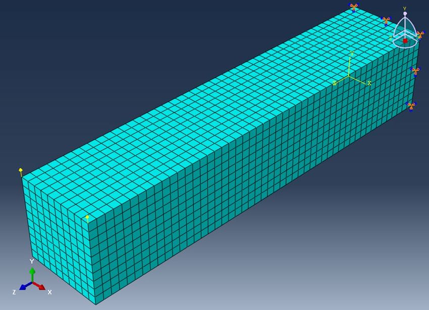
www.nature.com/scientificreports/
Figure 3. Spatial discretization of the W-element.
where {u} is the constant displacement on the surface of Su .
The other one is the surface traction boundary condition on the surface Sσ defined as
[n]{σ } = T on Sσ , (10)
� � �� T x
T x, y, z = T y , (11)
Tz
� � �� nx 0 0 ny 0 nz
n x, y, z = 0 ny 0 nx nz 0 , (12)
0 0 nz 0 ny nx
where
T
is the constant
surface traction force per area on Sσ , [n] is the orientation cosine matrix, nx x, y, z ,
ny x, y, z , and nz x, y, z are the orientation cosine of the outer normal vector of the surface Sσ.
The initial condition can be defined as
u x, y, z, t = u x, y, z when t = 0, (13)
u̇ x, y, z, t = u̇ x, y, z when t = 0, (14)
where {u} is the constant displacement of the domain when t = 0, u̇ is the constant velocity of the domain
when t = 0.
Coordinate mapping based on scaled boundary transformation. Taking one W-element as an
example (see Fig. 3), the boundary is discretized with one plane four nodes linear finite element with circumfer-
ential axis of η and ζ (see Fig. 4). Other 2D finite elements such as the quadratic element with eight nodes can be
used for this boundary discretization as well51.
The origin of the global Cartesian coordinate system of the nodes needs to be translated to the scaling center
by
{xe } = {x̃e } − x̃e0 ,
ye = ỹe − ỹe0 , (15)
{ze } = {z̃e } − z̃e0 ,
where {x̃e }, ỹe , and {z̃e } denote the global coordinates of the
nodes, x̃e0, ỹe0, and z̃e0 denote the coordinates of the
scaling center in global Cartesian coordinate system, {xe }, ye , and {ze } denote the translated global coordinates
of the nodes.
The mapping function between the global coordinates and the local coordinates of the points on the bound-
ary is given by
Scientific Reports | (2022) 12:4156 | https://doi.org/10.1038/s41598-022-07996-6 5
Vol.:(0123456789)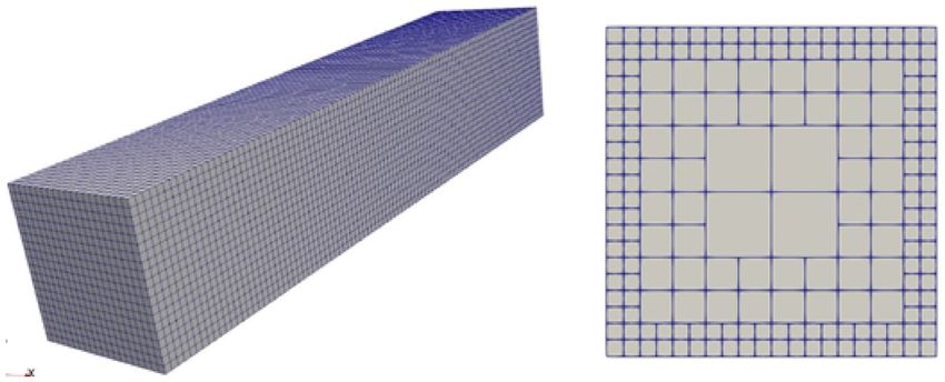
www.nature.com/scientificreports/
Figure 4. Four nodes linear plane finite element.
x̂(η, ζ ) = {N(η, ζ )}T {xe },
ŷ(η, ζ ) = {N(η, ζ )}T ye , (16)
T
ẑ(η, ζ ) = {N(η, ζ )} {ze },
where {N(η, ζ )} = N1 N2 N3 N4 denotes the shape function of the plane finite element, {xe }, ye , and {ze }
T
denote the global coordinates of the nodes that have been translated by Eq. (15), x̂(η, ζ ), ŷ(η, ζ ), and ẑ(η, ζ )
denote the global coordinates of arbitrary point on the boundary determined by the local coordinates (η, ζ ).
The new local scale boundary coordinate is built for this W-element with the origin at the scaling center.
Points on the plane finite element is scaled along the radical direction from the scaling center to the boundary,
which is defined as the ξ axis of the local scale boundary coordinate. The mapping function between the global
coordinates and the local coordinates of the points in the W-element is given by
x(ξ , η, ζ ) = ξ x̂ = ξ {N(η, ζ )}T {xe
},
y(ξ , η, ζ ) = ξ ŷ = ξ {N(η, ζ )}T ye , (17)
z(ξ , η, ζ ) = ξ ẑ = ξ {N(η, ζ )}T {ze },
where x(ξ , η, ζ ), y(ξ , η, ζ ), and z(ξ , η, ζ ) denote the local coordinates of the points in the W-element.
Equation (17) provides a mapping relation between the local and global coordinates. Based on the deriva-
tive method for compound function, the corresponding relationship of the derivative operators between two
coordinates is given by
∂
∂
∂x
∂ξ
∂ −1 ∂
∂y = [J] ∂η , (18)
∂
∂
∂z ∂ζ
where [J] is the Jacobian matrix expressed as
∂x ∂y ∂z
∂ξ ∂ξ ∂ξ
∂x ∂y ∂z
[J] = ∂η ∂η ∂η . (19)
∂x ∂y ∂z
∂ζ ∂ζ ∂ζ
The variable ξ can be isolated from Eq. (19) as
1 0 0
[J(ξ , η, ζ )] = 0 ξ 0 Ĵ , (20)
0 0 ξ
with the Jacobian matrix on the boundary Ĵ defined as
x̂ ŷ ẑ
Ĵ(η, ζ ) = x̂,η ŷ,η ẑ,η , (21)
x̂,ζ ŷ,ζ ẑ,ζ
where (·),η denotes differentiating with respect to η, (·),ζ denotes differentiating with respect to ζ.
Based on the space analytical geometric theory, the geometry properties in the local coordinate system can
be derived. The infinitesimal line vectors in the axis direction are given by
−
→
− →
−→
dξ = dξ x̂, ŷ, ẑ , dη = ξ dη x̂,η , ŷ,η , ẑ,η , dζ = ξ dζ x̂,ζ , ŷ,ζ , ẑ,ζ , (22)
where (·) denotes a vector.
The infinitesimal volume is given by
Scientific Reports | (2022) 12:4156 | https://doi.org/10.1038/s41598-022-07996-6 6
Vol:.(1234567890)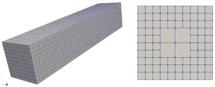
www.nature.com/scientificreports/
−
→ − → − →
dV = dξ · dη × dζ = ξ 2 Ĵ dξ dηdζ ,
(23)
where |·| denotes the determinant of the matrix.
The normal vectors of the coordinate surfaces are given by
−
→
g ξ = ŷ,η ẑ,ζ − ŷ,ζ ẑ,η , ẑ,η x̂,ζ − ẑ,ζ x̂,η , x̂,η ŷ,ζ − x̂,ζ ŷ,η ,
−
→
g η = ŷ,ζ ẑ − ŷ ẑ,ζ , ẑ,ζ x̂ − ẑ x̂,ζ , x̂,ζ ŷ − x̂ ŷ,ζ , (24)
−
→
g ζ = ŷ ẑ,η − ŷ,η ẑ, ẑ x̂,η − ẑ,η x̂, x̂ ŷ,η − x̂,η ŷ ,
−
→− → −
→
where g ξ , g η , and g ζ denote the normal vector of the coordinate surface of Sξ , S−
→and
η
−
→ Sζ. −
→
The length of the normal vectors g , g , and g and the unit normal vectors n , n , and nζ are defined as
ξ η ζ ξ η
−→ −
→
−
→
g = g , g = g , g = g ζ ,
ξ ξ η η ζ
(25)
−
→ −
→ −
→
−
→ gξ
−
→ gη
−
→ gζ
nξ = ξ = nξx , nξy , nξz , nη = η = nηx , nηy , nηz , nζ = ζ = nζx , nζy , nζz , (26)
g g g
where |·| denotes the length of the vector.
The infinitesimal area of the coordinate surfaces is given by
− →
→ −
dSξ = dη × dζ = ξ 2 g ξ dηdζ ,
− →
→ −
dSη = dζ × dξ = ξ g η dξ dζ , (27)
− →
→ −
dSζ = dξ × dη = ξ g ζ dξ dη.
−1
Ĵ can be expressed as
ξ η ζ
gξ n gηn gζ n
� �−1 1 ξ xξ η xη ζ xζ
Ĵ = ��� ��� g ny g ny g ny . (28)
� Ĵ � g ξ nξz g η nηz g ζ nζz
Substituting Eq. (28) into Eq. (18), the derivative operators in the local coordinates is given by
∂ gξ ξ ∂ 1 gη η ∂ gζ ζ ∂
= ��� ��� nx + �� �� n + ��� ��� nx ,
∂x � Ĵ � ∂ξ ξ �� Ĵ �� x ∂η � Ĵ � ∂ζ
∂ gξ ξ ∂ 1 gη η ∂ gζ ζ ∂
= ��� ��� ny + �� �� n + ��� ��� ny , (29)
∂y � Ĵ � ∂ξ ξ �� Ĵ �� y ∂η � Ĵ � ∂ζ
∂ gξ ξ ∂ 1 gη η ∂ gζ ζ ∂
= ��� ��� nz + �� �� n + ��� ��� nz .
∂z � Ĵ � ∂ξ ξ �� Ĵ �� z ∂η � Ĵ � ∂ζ
Substituting Eq. (29) into Eq. (7), the spatial partial derivative operator [L] in local coordinate system is given
by
1
∂ 1 2
∂ 3
∂
[L] = b + b + b , (30)
∂ξ ξ ∂η ∂ζ
where b1 , b2 , and b3 are defined as
ξ
nx 0 0
0 ξ
ny 0
ξ
� 1� gξ 0 0 nz
(31)
b = � � ξ
� � �� ξ ,
ny
� Ĵ � nx 0
ξ ξ
0 nz ny
ξ ξ
nz 0 nx
Scientific Reports | (2022) 12:4156 | https://doi.org/10.1038/s41598-022-07996-6 7
Vol.:(0123456789)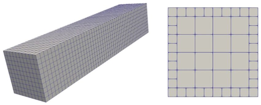
www.nature.com/scientificreports/
η
nx 0 0
η
0 ny 0
η
� 2� gη 0 0 nz
b = ��� ��� η η , (32)
� �
Ĵ ny nx 0
0 η η
nz ny
η η
nz 0 nx
ζ
nx 0 0
0 ζ
ny 0
ζ
� 3� gζ 0 0 nz
(33)
b = ��� ��� ζ ζ ,
ny
� Ĵ � nx 0
ζ ζ
0 nz ny
ζ ζ
nz 0 nx
and they satisfy
2
+
Ĵ
b3 = −2
Ĵ
b1 .
Ĵ
b
,η ,ζ
(34)
Substituting Eq. (30) into Eqs. (2) and (3), the stress {σ } in local coordinate system is given by
1
2
{σ (ξ , η, ζ )} = [D] b1 {u(ξ , η, ζ )},ξ + b {u(ξ , η, ζ )},η + b3 {u(ξ , η, ζ )},ζ . (35)
ξ
Considering the surface traction boundary condition in Eq. (10) to Eq. (12), the surface traction on the
coordinate surface is defined as
σx
n
ξ
0 0 n
ξ
0 n
ξ
σy
� �T x y z
� ξ� ξ ξ ξ ξ ξ ξ σz
t = tx ty tz = 0 ny 0 nx nz 0
τxy
, (36)
ξ ξ ξ
0 0 nz 0 ny nx
τ
yz
τzx
σx
η η η
σy
n x 0 0 ny 0 nz
� η � � η η η �T η η η σ z
t = tx ty tz = 0 ny 0 nx nz 0 , (37)
η η η τxy
0 0 nz 0 ny nx
τ
yz
τzx
σx
σy
ζ ζ ζ
� ζ � � ζ ζ ζ �T nx 0ζ 0 nyζ 0ζ nz σz
t = tx ty tz = 0 ny 0 nx nz 0
τxy
, (38)
ζ ζ ζ
0 0 nz 0 ny nx
τ
yz
τzx
where t ξ , {t η }, and t ζ denote the the surface traction on the coordinate surface of ξ , η, and ζ respectively.
Compared with Eq. (31) to Eqs. (33), (36) to Eq. (38) can be reformulated as
ξ
Ĵ
1 T
t = ξ b {σ }, (39)
g
η
Ĵ
2 T
t = η b {σ }, (40)
g
ζ
Ĵ
3 T
t = ζ b {σ }. (41)
g
Spatial discretization of the displacement field on the boundary. Taking the same W-element in
“Coordinate mapping based on scaled boundary transformation” section as example (see Fig. 5), the boundary
is discretized with a finite element with circumferential axis of η and ζ (see Fig. 4).
Scientific Reports | (2022) 12:4156 | https://doi.org/10.1038/s41598-022-07996-6 8
Vol:.(1234567890)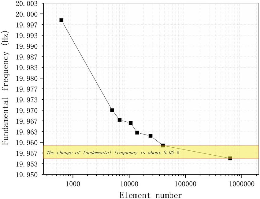
www.nature.com/scientificreports/

                                 Figure 5.  Displacement field discretization of the W-element.

                                    The displacement field on the boundary {u(η, ζ )} can be expressed as

                                                                             {u(η, ζ )} = [N(η, ζ )] ue ,                                       (42)

                                 where [N(η, ζ )] = N1 (η, ζ )[I] N2 (η, ζ )[I] N3 (η, ζ )[I] N4 (η, ζ )[I] denotes the shape function of the finite
                                 element, {ue } denotes the displacement values of the nodes, [I] denotes a 3 × 3 identity matrix.
                                    The interpolation shown in Eq. (42) is applied to any coordinate surface of Sξ . The displacement field
                                 {u(ξ , η, ζ )} in the W-element can be expressed as

                                                                          {u(ξ , η, ζ )} = [N(η, ζ )] ue (ξ ) ,                                 (43)
                                 where {ue (ξ )} denotes the the displacement values along the rays starting from the scaling center to the nodes
                                 on the boundary.
                                    Substituting Eq. (43) into Eq. (35), the discretization of the stress {σ } is given by

                                                                                              1
                                                                    {σ } = [D] B1 ue (ξ ) ,ξ + B2 ue (ξ ) ,                                  (44)
                                                                                                  ξ

                                 where B1 (η, ζ ) , B2 (η, ζ ) are defined as
                                                                                 1
                                                                                 B (η, ζ ) = b1 [N],                                         (45)

                                                                        2
                                                                        B (η, ζ ) = b2 [N],η + b3 [N],ζ .                                      (46)

                                 Equivalent integral equations and Galerkin weighted residual method. The SBFEM governing
                                 equation can be derived by the application of the weighted residual method or variation principle. In this sec-
                                 tion, the procedure of Galerkin weighted residual method is elaborated.
                                    The equivalent integral form of Eq. (7) is given by

                                                          T  1 T                  T 1  2 T       T
                                                           wj b {σ },ξ dV +           wj      b {σ },η + b3 {σ },ζ dV
                                                                                          ξ
                                                       V                          V

                                                                T

                                                                                     T                                                  (47)
                                                         −      wj ρ{ü}dV +         wj   p dV = {0},
                                                            V                    V
                                        T
                                 where
                                    w   j denotes the arbitrary weight function defined in Eq. (48), [·]T denotes the transpose of the matrix.
                                        T
                                    wj is defined as

Scientific Reports |   (2022) 12:4156 |               https://doi.org/10.1038/s41598-022-07996-6                                                  9

                                                                                                                                             Vol.:(0123456789)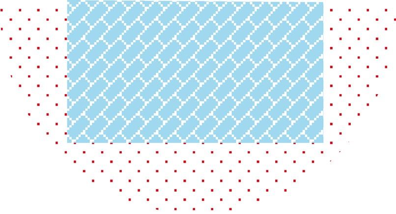
www.nature.com/scientificreports/
1 0 0
wj (ξ , η, ζ ) = wj [I] = wj 0 1 0 . (48)
0 0 1
where j = 1, 2, . . . , m denotes the number of weight functions and m → ∞.
Substituting Eq. (23) into Eq. (47) results in
I
1 1 1
T 1 T
ξ2
wj b {σ },ξ Ĵ(η, ζ ) dηdζ dξ
0 −1 −1
II
1
1 1 T 1 2 T
T
ξ2 wj ξ b {σ },η + b3 {σ },ζ Ĵ(η, ζ ) dηdζ dξ
+
−1 −1
0
III
(49)
1 1 1
2
T
+ ξ wj p Ĵ(η, ζ ) dηdζ dξ
0 −1 −1
IV
1 1 1
T
ξ2
− wj ρ{ü} Ĵ(η, ζ ) dηdζ dξ = {0}.
0 −1 −1
Dealing the second term labeled II in Eq. (49) with Green’s theorem results in
�1
�1 �1 � �T �� 2 �T � �T ��� ��
b {σ },η + b3 {σ },ζ � Ĵ(η, ζ ) �dηdζ dξ
� �
II = ξ wj
−1 −1
0
�1 �� � �T �� 2 �T � �T ��� ��
b {σ },η + b3 {σ },ζ � Ĵ(η, ζ ) �dηdζ dξ
� �
= ξ wj
Sξ (50)
0
� � �T ����� ���� 2 �T �
��� ��� �
T
� �
� Ĵ � b {σ } dζ + � Ĵ � b3 {σ } dη
� �
�1 wj
Ŵξ
= ξ
��
�� �� � �� ��� � �
T� � 2 T
�� � �� ��� � � � �
T� T
dξ ,
+ wj � Ĵ � b3
�
0
− wj � Ĵ � b {σ } dηdζ
,η ,ζ
Sξ
where Γ ξ denotes the the boudnary of surafce Sξ.
Substituting Eq. (39) to Eq. (41) into Eq. (50) results in
� � �T ���� ���� 2 �T �� ��� � �
T
� Ĵ � b {σ }dζ + � Ĵ � b3 {σ }dη
� �
�1 wj
�Ŵ ξ
II = ξ
�� �� �T ��� ���� 2 �T � �� � �� ��� � � �
T� T
dξ
wj � Ĵ � b3
�
0
− w j � Ĵ � b + {σ }dηdζ
,η ,ζ
Sξ
� � �T � η η � � �
wj {t }g dζ + t ζ g ζ dη
1 ξ
�
� �TŴ���� ���� �T � � �T ��� ���� 2 �T
= ξ w Ĵ b 2 + wj ,η � Ĵ � b dξ
j � �
(51)
��
− � � ��� ��� � �,η � �T ��� ���� 3 �T {σ }dηdζ
0 T � � 3 T
Sξ + wj � Ĵ � b + wj ,ζ � Ĵ � b
,ζ
� � �T � η η � � �
wj {t }g dζ + t ζ g ζ dη
�1 �Ŵξ ��� ��� � � �
� �T ���� ���� 2 �T � T
= ξ
�� wj � Ĵ � b + � Ĵ � b3
� �
dξ ,
,η
0
− � � �� ��� � � � �� ��� � ,ζ {σ }dηdζ
T T T T
+ wj ,η � Ĵ � b2 + wj ,ζ � Ĵ � b3
Sξ
� � � �
where the surface traction boundary condition {t η } and t ζ is introduced naturally.
Substituting Eq. (34) into Eq. (51) results in
Scientific Reports | (2022) 12:4156 | https://doi.org/10.1038/s41598-022-07996-6 10
Vol:.(1234567890)www.nature.com/scientificreports/
� � �T � η η � � �
wj {t }g dζ + t ζ g ζ dη
�1 �Ŵξ ��� ��� � � �
� �T ���� ���� 2 �T � � � 3 T
II = ξ �� wj � Ĵ � b + � Ĵ � b dξ
− � � �� ,η � � �� ,ζ {σ }dηdζ
0 � � T � �T � � T � � T
+ wj ,η � Ĵ � b2 + wj ,ζ � Ĵ � b3
Sξ
� � � �
� � �T � η η � � �
wj {t }g dζ + t ζ g ζ dη
�1 ξ
� � �Ŵ �� ��� � � � � �� ��� �
=
ξ �� T � � 1 T T� � 2 T
dξ (52)
− wj −2 � Ĵ � b + w j ,η � Ĵ � b
0 � �T�
� � �� � � T
{σ }dηdζ
+ wj ,ζ � Ĵ � b3
�
Sξ
� � �T � η η � � �
wj {t }g dζ + t ζ g ζ dη
�1 ξ
� Ŵ �
= ξ �� −2�w �T �b1 �T + �w �T �b2 �T �� �� dξ .
− j j ,η � �
0 � � T � � T {σ } � Ĵ �dηdζ
Sξ + wj ,ζ b3
Substituting Eq. (52) into Eq. (47), the equivalent integral weak form of Eq. (47) is given by
1 1
2
T
1
T
ξ wj b {σ },ξ
Ĵ
dηdζ
−1 −1
T η η
+ξ wj {t }g dζ + t ζ g ζ dη
Ŵξ
1
1
T
T
T
T
T
T
−ξ −2 wj b1 + wj ,η b2 + wj ,ζ b3 {σ }
Ĵ
dηdζ (53)
−1
−1
1 1
2
T
+ξ wj p
Ĵ
dηdζ
−1 −1
1 1
2
T
−ξ wj ρ{ü}
Ĵ
dηdζ = {0},
−1 −1
where the surface traction boundary condition {t η } and t ζ is introduced naturally, Ŵ ξ denotes the the boudnary
of surafce Sξ.
By applying the weighted residual method, the arbitrary weight function wj in Eq. (53) is simplified to a
particular weight function {w}, the approximate form of Eq. (53) is given by
1 1
T
ξ2 {w}T b1 {σ },ξ
Ĵ
dηdζ
−1 −1
+ξ {w}T {t η }g η dζ + t ζ g ζ dη
Ŵξ
1
1
T
T
T
−ξ −2{w}T b1 + {w}T,η b2 + {w}T,ζ b3 {σ }
Ĵ
dηdζ (54)
−1
−1
1 1
2
+ξ {w}T p
Ĵ
dηdζ
−1 −1
1 1
− ξ2 {w}T ρ{ü}
Ĵ
dηdζ = {0},
−1 −1
where denotes the weight functions in the W-element, {·}T denotes a row vector.
{w}T
Considering the Galerkin weighted residual method, the interpolation of {w}T is the same as {u(ξ , η, ζ )} in
Eq. (43) as
{w(ξ , η, ζ )} = [N(η, ζ )] w e (ξ ) . (55)
Scientific Reports | (2022) 12:4156 | https://doi.org/10.1038/s41598-022-07996-6 11
Vol.:(0123456789)www.nature.com/scientificreports/
Substituting Eq. (43), Eqs. (29) and (55) into Eq. (54), the SBFEM governing equation in the time domain
for 3D elastic continuum media is given b y53
0
2
T
T
E ξ {u},ξ ξ + 2 E 0 − E 1 + E 1 ξ {u},ξ + E 1 − E 2 {u}
(56)
− M 0 ξ 2 üe (ξ ) + ξ {T} + ξ 2 {P} = {0},
where the constant coefficient matrix is given by
1
1
0
T
E = B1 [D] B1
Ĵ
dηdζ ,
−1 −1
1
1
T
E1 = B2 [D] B1
Ĵ
dηdζ ,
−1 −1
(57)
1
1
2
2 T
E = B [D] B2
Ĵ
dηdζ ,
−1 −1
1
1
0
[N]T ρ[N]
Ĵ
dηdζ .
M =
−1 −1
The governing equation of W-elements sharing the same scaling center can be assembled by the degree of
freedom contributed by adjacent W-elements,
which
results
in the governing equation of the S-element like
Eq. (56) but with the assembled {u}, E 0 , E 1 , E 2 , and M 0 .
Solution of the SBFEM governing equation. The SBFEM governing equation (Eq. (56)) is a system of
second order Ordinary Differential Equations (ODEs) called the Euler-Cauchy equations. The solution of this
system is given in a closed form. The first step is to introduce a dual variable to convert the system of second
order ODEs to a system
of
one order with variables doubled in size. Based on the principle of virtual work, the
internal node force q(ξ ) along
the ray starting from the scaling center to the nodes on the boundary resulting
from the surface traction t ξ on the coordinate surface of Sξ is given by
{w(ξ )}T q(ξ ) = {w(ξ , η, ζ )}T t ξ (ξ , η, ζ ) dSξ ,
(58)
Sξ
T
q(ξ ) = E 0 ξ 2 {u(ξ )},ξ + E 1 ξ {u(ξ )}. (59)
If the body forces vanish, Eq. (56) can be reformulated as
ξ {X(ξ )},ξ = [Z]{X(ξ )}. (60)
where
ξ 0.5 {u(ξ )}
{X(ξ )} =
ξ −0.5 q(ξ )
, (61)
and
−1
1
T
0
−1
0.5[I] − E 0 E E
[Z] =
2
1
0
−1
1
T
1
0
−1 . (62)
E − E E E E E − 0.5[I]
The eigenvalues and eigenvectors of the matrix [Z] can be obtained by
[Z][�] = [�][ ], [ ] = diag( 1 , 2 , . . . , 2n ), (63)
where [�] = {φ1 } {φ1 } . . . {φ2n } denotes a matrix consisted of the eigenvectors {φ1 }, {φ1 }, . . . , {φ2n },
1 , 2 , . . . , 2n denotes the eigenvalues, diag(·) denotes a diagonal matrix. It is worth to notice that the eigenval-
ues in [ ] should be in descending order, so the eigenvectors in [ ]. The eigenvectors {φ1 }, {φ1 }, . . . , {φ2n } and
the eigenvalues 1 , 2 , . . . , 2n can be partitioned into two blocks as
u
[ ] =
bq
, (64)
b
Scientific Reports | (2022) 12:4156 | https://doi.org/10.1038/s41598-022-07996-6 12
Vol:.(1234567890)www.nature.com/scientificreports/
[ u ] [0u ]
[ ] = q q
[0 ] [ ]
, (65)
where the subscript u denotes the block related to {u(ξ )}, the subscript q denotes the block related to q(ξ ) .
The solution of Eq. (60) considering boundary conditions is given by
{u(ξ )} = ξ −0.5 �ub ξ b {c}, (66)
q
q(ξ ) = ξ 0.5 �b ξ b {c}, (67)
T
where {c} = c1 c2 · · · cn denotes the arbitrary integration constant, ξ b denotes a diagonal matrix expressed
as
ξ 1 0 · · · 0
. .
0 ξ 2 . . ..
ξ b =
. .
, (68)
.. ... 0
..
0 · · · 0 ξ n
For the SBFEM polyhedron element, the coefficient matrix representing the stiffness and mass matrix of
the S-element need to be derived. Substituting Eq. (67) into Eq. (66) to eliminate {c}, the stiffness matrix [K] is
given by51
q
−1
[K] = b ub , (69)
where [·]−1 denotes the inverse of the matrix.
Based on the virtual work statement, the mass matrix [M] of the S-element can be expressed a s51
−T
−1
[M] = ub [m] ub , (70)
where [·]−T denotes the inverse of the transpose of the matrix, the value mij in the row i and column j of [m] is
defined as
m0ij
[m] = mij = , (71)
bi
+ bj + 2
where the m0ij is the value in the row i and column j of m0 defined as
−T 0
u
−1
m0ij = m0 = ub M b . (72)
Topology and data structure of an arbitrary polyhedron element
The polyhedron geometry is a 3D shape with straight edges, sharp corners and vertices, and any number greater
than 2 of plane polygonal faces with any number greater than 2 of straight edges and vertices. The tetrahedron,
pentahedron, hexahedron and heptahedron that widely used in FEM are just the special cases of the convex
polyhedron. Vastly different from the FEM element geometry, the first step to construct a polyhedron element
is to describe the uncertainty of the topology of varied kinds of polyhedron elements in a model with a uniform
data structure that can be recorded in the intermediate file for compatible purpose.
Essential information to describe the topology of an arbitrary polyhedron. For example, Fig. 6
shows a polyhedron element that may be encountered in an octree mesh, which has nine facets, twenty edges and
thirteen vertices. The coordinates of the vertices are the basic information as shown in Table 1. In addition, the
connectivity of the vertices of each facet needs to be defined as shown in Table 2. These two sets of information
are sufficient and necessary for the description of the topology of any polyhedron. It is worth to notice that the
order of the vertices and facets of a polyhedron is insignificant and when there are multiple polyhedra, there is
no need to record the correspondence between the local and global vertex ID like FEM.
SBFEM discretization of the polyhedron. The geometry of the S-element can be adapted for any con-
vex polyhedron with only triangle or quadrilateral facets which is a special case of the polyhedron defined in
“Essential information to describe the topology of an arbitrary polyhedron” section. Nevertheless, the polygonal
facet of a polyhedron can always be converted into multiple triangle or quadrilateral facets by adding a vertex on
this facet (see Fig. 6). After this treatment of the polyhedron facets, a point inside the polyhedron that can see
all the points on the facets is chosen as the scaling center and the vertices are defined as nodes of this polyhe-
dron domain. The scaling center and the nodes of each facet constitute a W-element. All these W-elements are
assembled into an S-element representing this polyhedron domain. It is obvious that the number of W-elements
is equal to the number of facets of the polyhedron and the number of the nodes of the S-element is equal to the
number of vertices of the polyhedron. The data structure to describe any 3D SBFEM polyhedron element is
summarized in Table 3.
Scientific Reports | (2022) 12:4156 | https://doi.org/10.1038/s41598-022-07996-6 13
Vol.:(0123456789)www.nature.com/scientificreports/
Figure 6. Topology of a polyhedron element and the treatment of the polygon facet.
Vertex ID X coordinates Y coordinates Z coordinates
1 0.0 0.0 0.0
2 0.0 10.0 0.0
3 10.0 10.0 0.0
4 10 5.0 0.0
5 10.0 0.0 0.0
6 10.0 10.0 5.0
7 10.0 5.0 5.0
8 10.0 0.0 5.0
9 0.0 0.0 10.0
10 0.0 10.0 10.0
11 10.0 10.0 10.0
12 10.0 5.0 0.0
13 10.0 0.0 10.0
Table 1. Vertex information of the polyhedron element.
Facet ID Vertex connectivity
1 1, 2, 3, 4, 5
2 9, 13, 12, 11, 10
3 2, 10, 11, 6, 3
4 1, 9, 10, 2
5 1, 5, 8, 13, 9
6 7, 6, 11, 12
7 8, 7, 12, 13
8 4, 3, 6, 7
9 5, 4, 7, 8
Table 2. Facet information of the polyhedron.
Scientific Reports | (2022) 12:4156 | https://doi.org/10.1038/s41598-022-07996-6 14
Vol:.(1234567890)www.nature.com/scientificreports/
Element ID k
Coordinate of scaling center x0, y0, z0
Number of facets m
Number of nodes n
Local node ID Global node ID Node coordinates
1 N1 x1, y1, z1
2 N2 x2, y2, z2
… … …
n Nn xn, yn, zn
Facets Number of nodes Node conectivitya
1 J1 N11, N12, …,N1J1
2 J2 N11, N12, …,N1J2
… … …
m Jm Nm1, Nm2, …,NmJm
Density ρk
Young’s modulus Ek
Poisson’s ratio vk
Table 3. Data structure of the SBFEM polyhedron element. a The node sequence should be in a certain order
pointing out of the region according to the right-hand rule.
Generation of the SBFEM polyhedron mesh. There are roughly three kinds of tools to obtain a poly-
hedron mesh: the self-developed program, the open-source or commercial mesh generator. Liu et al. brought up
an automatic octree mesh generation algorithm from an STL geometry file in MATLAB for three-dimensional
domain38. Besides, at present OPENFOAM, FLUENT and STAR-CCM + provide robust polyhedron mesh gen-
erators, the latter two of which are the most convenient. The general procedure to generate a polyhedron mesh
from geometry with an out-of-box tool is illustrated in Fig. 7. Because the common FEM software for solid media
does not support the polyhedron element, the preprocessor built in them cannot generate polyhedron meshes.
Furthermore, the raw polyhedron mesh needs some extra processing steps such as classification, grouping, add-
ing vertices before applied. The flow of geometry and mesh information between various software through files
in compatible formats is inevitable. The Initial Graphics Exchange Specification (IGES) for the geometry infor-
mation and Visualization Toolkit (VTK) for the mesh information are recommended. It should be noted that no
matter which polyhedron mesh generator above is chosen or developed, it is required to store the polyhedron
mesh in the intermediate file that will be imported into the UEL after the polyhedron mesh is obtained.
Implementation in ABAQUS
The SBFEM polyhedron element is introduced in ABAQUS/Standard as a user element. The user element is
implemented on the element iteration level of the solver in the form of a FORTRAN subroutine named UEL.
During each increment of the computation, ABAQUS will invoke the UEL when calculating the coefficient
matrix of each user element on and on until the end of the analysis. Assembly of the global coefficient matrix,
nonlinear iteration, result output, imposition of contact, constrain, boundary and load conditions are performed
by ABAQUS automatically.
Basics of UEL in ABAQUS. UEL is essentially a function to compute specific variables with given vari-
ables. The subroutine name, declaration of the input and output variables are fixed (see “Appendix 1”54). During
the calculation of each element, the UEL will be called importing information of analysis type, time increment,
element type, right-hand-side vectors, etc. to export the mass matrix, stiffness matrix, equivalent nodes force
vector, solution-dependent state variables, etc.
There are some conventions of user subroutines in ABAQUS that should be emphasized. All user subroutines
and the subroutines created by users must be stored in a single source code file or its compiled object file. By
default, the user subroutine can call another subroutine that is built in FORTRAN compiler, created by users or
provided by ABAQUS named utility routines. This restriction suggests that some complicated calculations in
a user subroutine have to be implemented by source codes provided by users. And if there were multiple user
elements, these user elements should be implemented by the same subroutine of UEL with conditional branch
statements on element types. Although user subroutines cannot call each other, the data can be transferred
through the user-defined COMMON block variables between them.
Associated INP and intermediate file. A convenient characteristic of ABAQUS is that the entire infor-
mation of a FEM model is stored in an INP file, which is human-readable. This INP file is the only input required
by the solver of ABAQUS. The user elements must be declared in the INP file before the calculation (see “Appen-
dix 2”54). The declaration of user elements provide the information of the element type, element set name, num-
ber of nodes, node connectivity, node degrees of freedom and element properties such as material parameters,
etc. According to the format of the user element declaration in an INP file, the user elements need to be classified
Scientific Reports | (2022) 12:4156 | https://doi.org/10.1038/s41598-022-07996-6 15
Vol.:(0123456789)www.nature.com/scientificreports/
Figure 7. General procedure of SBFEM polyhedron mesh generation by out-of-box tools.
into different types based on at least the number of nodes and the material properties and the node connectivity
of polygonal facets of a polyhedron cannot be represented.
Due to the limitation of the INP file mentioned before, an intermediate file storing the topology information
and material properties of arbitrary polyhedron elements is necessary. This file should be imported once the
calculation is started and when iterating through the elements, the corresponding topology information of cur-
rent user element should be introduced into UEL. With this intermediate file, any polyhedron mesh generator
mentioned in “Generation of the SBFEM polyhedron mesh” section can be used and any mesh with arbitrary
convex polyhedron shape can be calculated.
Algorithm of UEL for SBFEM polyhedron element. Although UEL has provided a specific interface,
it is necessary to understand the calculation process of ABAQUS/Standard to get a clear picture of what infor-
mation is passed in UEL and what information UEL should return under different circumstances. As shown
in Fig. 8, calculation process of ABAQUS/Standard has a hierarchy of three levels. Level 1 denotes the calcula-
tion procedure of steps in an analysis. Level 2 denotes the calculation procedure of increments of a step. Level
3 denotes the actual calculation of the polyhedron element matrix and vector in an increment by calling UEL
for each element (see the green block in Fig. 8). The utility routine of UEXTERNALDB plays an important role
in Level 1 and 2 (see the red blocks in Fig. 8), providing adequate interventions into the different phases of the
calculation process, which give us more freedom to realize more complex functions. To coincide with UEL, the
intermediate file storing the topology and material information of user polyhedron elements is imported by
subroutine UEXTERNALDB at the beginning of the analysis, which is then transferred into UEL by COMMON
block variables when the calculation of the polyhedron element starts.
The behavior of UEL is controlled by the basic branching structure (see Fig. 9) judged by the variable of
LFLAGS. Considering only the general static and direct-integration dynamic analysis, there are five different
cases (see colored blocks in Fig. 9) requiring returned values respectively according to the Newton–Raphson
Method (NRM) and HHT direct time i ntegration55.
The polyhedron element computation algorithm of UEL based on SBFEM is summarized in “Appendix 3”.
The assembly of the coefficient matrix of W-elements in STEP 2.3 and stiffness and mass matrix calculation that
Scientific Reports | (2022) 12:4156 | https://doi.org/10.1038/s41598-022-07996-6 16
Vol:.(1234567890)www.nature.com/scientificreports/
Figure 8. Hierarchy of the calculation process of ABAQUS/Standard.
include Eigen-decomposition are the major differences from FEM. Subroutines from LAPACK56 is appended
to UEL in the code file to perform STEP 3. It is obvious that this UEL is compatible with the traditional FEM
element topology built in ABAQUS, considering the tetrahedron, pentahedron and hexahedron as special cases
of the polyhedron.
Numerical application
There are two examples for the test and application of the implementation of arbitrary polyhedral elements
developed in “Implementation in ABAQUS” section. A cantilever subjected to a harmonic excitation with the
traditional hexahedron element and the polyhedron element are compared to confirm the accuracy of the devel-
oped UEL. Then the polyhedron element based on SBFEM is applied in the soil-structure dynamic interaction
analysis of a nuclear power plant, the applicability and performance of this implementation is tested.
Cantilever subjected to a harmonic excitation. A 5 m long horizontal beam subjected to concentrated
forces on the vertices at one end and fixed at the other end is considered (see Fig. 10). The homogenous elastic
material properties of Young’s modulus, density and Poisson’s ratio are 20 GPa, 2000 kg/m3, and 0.25 respec-
tively. The harmonic concentrated forces in Y direction on the two vertices follow Eq. (73) defined as
2π
F = A sin t , (73)
T
Scientific Reports | (2022) 12:4156 | https://doi.org/10.1038/s41598-022-07996-6 17
Vol.:(0123456789)www.nature.com/scientificreports/
Figure 9. Basic branching structure of UEL for general static and direct-integration dynamic analysis.
Figure 10. Geometry, load and boundary conditions of the cantilever.
where T denoting the period is assuemd to be 0.05 s, A denoting the amplitude is assumed to be 1000 N. F
denotes the concentrated force. The HHT direct time integration calculation is terminated at 0.25 s with a fixed
time step of 0.001 s.
Numerical model. From the geometry, two sets of meshes with varied mesh density are generated. The first
set of meshes is made of structured hexahedron elements, namely C3D8 element (3D linear solid element with
8 nodes) built and verified in ABAQUS/Standard and the other is made of unstructured polyhedron elements
implemented by UEL based on SBFEM. The details of the meshes are summarized in Table 4, where label P1 to
P4 denote the polyhedron meshes with different mesh density (see Fig. 11) that can only be calculated by UEL
developed in “Implementation in ABAQUS” section and H1 to H7 denote the hexahedron meshes (see Fig. 12)
that can be calculated by C3D8 (built-in element) or the UEL (labeled as H2_UEL and H6_UEL). Model analysis
for the first 50 modes of vibration and implicit dynamic analysis are performed.
Scientific Reports | (2022) 12:4156 | https://doi.org/10.1038/s41598-022-07996-6 18
Vol:.(1234567890)www.nature.com/scientificreports/
Model name Element number Node number Mesh type Element type
P1 2312 4663 Polyhedron UEL
P2 4384 5977 Polyhedron UEL
P3 17,880 28,103 Polyhedron UEL
H1 5 24 Hexahedron C3D8
H2 40 99 Hexahedron C3D8
H3 117 224 Hexahedron C3D8
H4 153 288 Hexahedron C3D8
H5 625 936 Hexahedron C3D8
H6 5000 6171 Hexahedron C3D8
H7 625,000 652,851 Hexahedron C3D8
H2_UEL 40 99 Polyhedron UEL
H6_UEL 5000 6171 Polyhedron UEL
Table 4. Mesh information of the cantilever.
Results and discussion. Model analysis checking the stiffness and mass matrix with specific boundary condi-
tions is the most convenient approach to verify the user element for dynamic analysis, excluding the influence of
load conditions and nonlinearity. The results of the first 50 natural frequencies and the displacement response of
the dangling end (see Fig. 10) are compared to check the accuracy and efficiency of the UEL for the polyhedron
element. As the increasing of the number of elements, the results of model analysis will converge to the true value
of this problem. The first 50 natural frequencies of model H1 to H7 are listed in Fig. 13, from which the conver-
gence values of the first 50 natural frequencies of the cantilever are obtained covering more than 95% effective
mass in the main direction (97.1% in X and Y direction, 95.1% in Z direction).
Figure 13 shows that the difference between the frequencies of models with varied mesh densities is no more
than 9% for the first vibration mode and this difference is enlarged to less than 19% for the first 9 vibration modes,
which tends to keep on increasing with the order. Even though when the mesh is coarse, the convergence speed
is fast with the increasing of the element, the convergence speed is much slower near the convergence values
leading to rather poor computation efficiency (see Fig. 14). For example, the highest frequency of model H6
and H7 are 1374.8 Hz and 1392 Hz, the computation times of which are 5 s and 1109 s. More than 220 times the
computation time of model H6 brings less than 1.2% improvement of the results of model H7. This is a typical
illustration of the need to pay great attention to the balance between mesh density and calculation efficiency.
Since it is reasonable to assume that the results of model H7 are close enough to the convergence values, the true
fundamental frequency of this cantilever is assumed to be 19.955 Hz.
To exclude the influence of the meshes, the same hexahedron meshes H2 and H6 are calculated by C3D8
and UEL respectively. Figure 15 shows the frequency comparison of the cantilever model H6_UEL calculated
by UEL and H7 by C3D8. The consistency of the results of model H7 and H6_UEL confirms the accuracy of the
UEL for the SBFEM-based polyhedron element with error less than 0.6% over the entire calculated frequency
range. Figure 16 shows the frequency comparison of the cantilever mesh model H2 calculated by C3D8 and
UEL. Compared to model H2 calculated by C3D8, model H2_UEL can get much better results that is almost
equal to model H6 calculated by C3D8. In other words, polyhedron element based on SBFEM can get the same
level of accuracy with less than 1% of the elements based on FEM, the most immediate advantage of which is
the reduction in storage space for large-scale problems.
The displacement responses in Y direction from the implicit dynamic analysis of model P1, P2, P3, and H6
are demonstrated in Fig. 17. Except the displacement values that are close to zero, the error between the model
calculated by the C3D8 element and the user-defined polyhedron element based on SBFEM is less than 0.5%.
The results of model analysis and direct dynamic analysis of the cantilever have proven the accuracy of the UEL
implementation of the SBFEM-based polyhedron element and the efficiency of the SBFEM for the solid medium.
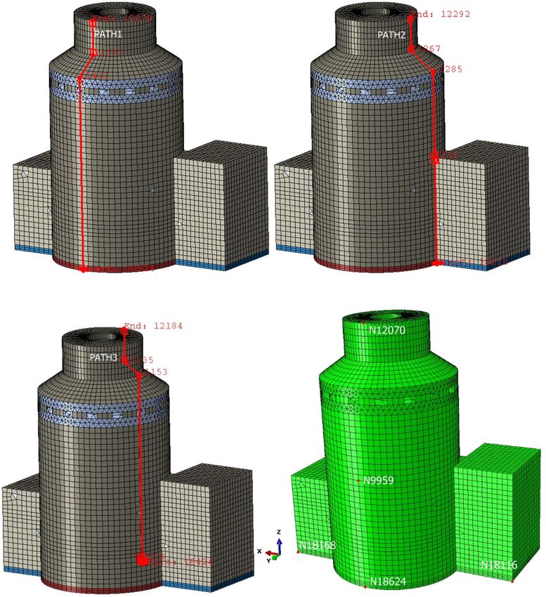
Soil‑structure dynamic interaction analysis of a nuclear power plant. To verify the performance
and robustness of the implementation that has been primarily validated in “Cantilever subjected to a harmonic
excitation” section, the application in the analysis of a practical engineering problem is necessary. A typical
numerical elastic SSI analysis of a NPP with direct method in the time domain is taken as an example, which
includes the simulation of the structure with traditional FEM elements, near field soil with the polyhedron
elements, far field soil with an artificial non-reflecting boundary condition, external excitation input with site
response analysis, and interaction between them with constrain or contact. For simplicity, the SSI analysis of a
NPP is elastic. But it is enough to demonstrate the merit in automatic mesh generation and ability to be inte-
grated seamlessly with other modules of the polyhedron element based on SBFEM and its implementation by
UEL. The nuclear power plant is located on elastic rock soil with the Young’s modulus of 2.63E10 Pa, Poisson’s
ratio of 0.25 and density of 1762.06 kg/m3. Two artificial seismic plane waves vibrating along the two horizontal
directions with PGA of 0.9806 m/s2 or 0.1 g (see Fig. 18) defined by the U.S. NRC RG 1.6057 response accelera-
tion spectrum (see Fig. 19) are introduced into the SSI system from the bottom of the rock propagating upward
along the vertical direction. This earthquake intensity just satisfies the minimum limit recommended by the
Scientific Reports | (2022) 12:4156 | https://doi.org/10.1038/s41598-022-07996-6 19
Vol.:(0123456789)You can also read