How to search for mirror stars with Gaia - Springer
←
→
Page content transcription
If your browser does not render page correctly, please read the page content below
Published for SISSA by         Springer
                                                                    Received: February 7,   2022
                                                                        Revised: May 18,    2022
                                                                       Accepted: June 2,    2022
                                                                      Published: July 11,   2022

How to search for mirror stars with Gaia

                                                                                                   JHEP07(2022)059
Aaron Howe,a Jack Setford,a David Curtina and Christopher D. Matznerb
a
  Department of Physics, University of Toronto,
 McLennan Physical Laboratories, 60 St George St, Toronto, ON M5S 1A7, Canada
b
  Department of Astronomy & Astrophysics, University of Toronto,
 50 St George St, Toronto, ON M5S 3H4, Canada
    E-mail: aaron.howe@mail.utoronto.ca, jsetford@physics.utoronto.ca,
    dcurtin@physics.utoronto.ca, matzner@astro.utoronto.ca

Abstract: We show for the first time how to conduct a direct search for dark matter using
Gaia observations. Its public astrometric data may contain the signals of mirror stars, exotic
compact objects made of atomic dark matter with a tiny kinetic mixing between the dark
and SM photon. Mirror stars capture small amounts of interstellar material in their cores,
leading to characteristic optical/IR and X-ray emissions. We develop the detailed pipeline
for conducting a mirror star search using data from Gaia and other stellar catalogues, and
demonstrate our methodology by conducting a search for toy mirror stars with a simplified
calculation of their optical/IR emissions over a wide range of mirror star and hidden sector
parameters. We also obtain projected exclusion bounds on the abundance and properties of
mirror stars if no candidates are found, demonstrating that Gaia is a new and uniquely
powerful probe of atomic dark matter. Our study provides the blueprint for a realistic
mirror star search that includes a more complete treatment of the captured interstellar gas
in the future.

Keywords: Models for Dark Matter, Particle Nature of Dark Matter, Hierarchy Problem

ArXiv ePrint: 2112.05766

Open Access, c The Authors.
                                                     https://doi.org/10.1007/JHEP07(2022)059
Article funded by SCOAP3 .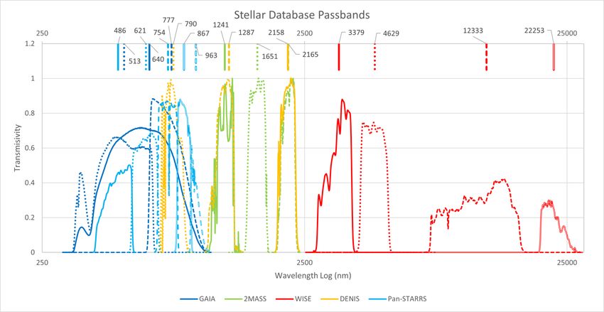
Contents

1 Introduction and motivation                                                                   1

2 Mirror star properties                                                                        3

3 Search for toy mirror stars                                                                   5
  3.1 Defining a mirror star signal region                                                      6
  3.2 Identifying mirror star candidates                                                        8

                                                                                                     JHEP07(2022)059
  3.3 Examination of candidates #1, #2 and #3                                                  12

4 Constraining mirror stars                                                                   15
  4.1 Warm-up: constraining a symmetric mirror sector                                         16
  4.2 Constraining mirror star abundance as a function of “mirror red dwarf”
      properties                                                                               21

5 Discussion and conclusion                                                                   23

1   Introduction and motivation

The Gaia telescope [1] has already measured the positions and velocities of well over a
billion stars, ushering in a new era of precision astronomy. Gaia’s unprecedented boon
of astrometric data also has tremendous potential to elucidate the nature of dark matter.
The velocity distribution of stars in tidal streams or in the stellar disk and halo provides
information on the Milky Way halo gravitational potential [2, 3] and certain features of
the dark matter spatial distribution [4–6], and investigations that were underway prior to
Gaia [7, 8] are now vastly accelerated [4]. Such analyses indirectly constrain dark matter
via its gravitational effects on stars. However, Gaia’s large catalogue of astrometric data
also allows for direct dark matter searches in more exotic and complex dark sectors. In this
paper, we develop the methodology to search for the optical and infrared emissions of mirror
stars [9, 10] made of atomic dark matter [11–27], using public data from the Gaia satellite
and other stellar catalogues. We also show how to obtain exclusions on the abundance and
detailed properties of mirror stars in the event that no candidates are observed.
     Complex dark sectors are highly motivated. From a bottom-up point of view, it is clear
that SM baryonic matter is extremely non-minimal, with many forces and particle species
that make up O(10%) of the matter in our universe. Therefore, in contrast to the hypothesis
of a single collisionless dark matter particle, it is plausible that parts of the remaining matter
are equally interesting. Atomic dark matter [11–27] postulates that dark matter contains at
least two states with different masses and opposite charge under a dark electromagnetism
U(1)D gauge symmetry. From a top-down point of view, many theories of Beyond-SM

                                              –1–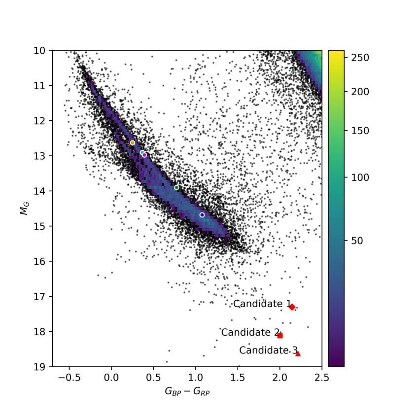
(BSM) particle physics postulate the existence of dark sectors related to the SM via discrete
symmetries [28–42]. Notably, this includes models of “neutral naturalness” such as the
Mirror Twin Higgs that address the hierarchy problem of the Higgs boson mass [28–35]
and could resolve outstanding anomalies in precision cosmology, see [43] (and also [26, 27]).
This can result in a fraction of dark matter being made up of dark baryons, with dark
protons, dark electrons, dark photons, and even dark nuclear forces that are similar to their
SM counterparts but with possibly different values for masses and interaction strengths.
     The observational consequences of this dark complexity are striking. A . 10% subcom-
ponent of dark matter that is made up of various dark particle species with sizeable self-
interactions would be compatible with cosmological and self-interaction bounds [16, 19, 33].

                                                                                                JHEP07(2022)059
Just as Standard Model (SM) particles like protons and electrons interact via electro-
magnetism, which allows baryonic gas to cool and form structure, these dark particles
could interact via dark electromagnetism, emitting (to us) invisible dark photons. The
resulting dissipation leads to the formation of dark structure, such as a dark disk or dark
microhalos [16, 17, 21], and mirror stars [9, 10, 39, 40, 44].
     It has recently been shown [9, 10] that mirror stars can produce electromagnetic signals
that may be visible in optical/IR and X-ray telescopes. This is possible if the dark photon
γD and the SM photon γ have a small kinetic mixing in the Lagrangian L ⊃ Fµν FDµν [45].
This small renormalizable operator is readily generated from many possible loop-processes
in the full UV-theory, with cosmological constraints [46] and estimates of gravitational
effects [47] motivating 10−13 .  . 10−9 . Such a tiny interaction has negligible effects
on cosmology, structure formation or astrophysics, but it does result in SM matter (dark
sector matter) acquiring a “dark milli-charge” (SM milli-charge). As a result, mirror stars
in our galaxy would capture a small amount of regular gas from the interstellar medium,
which sinks to the star’s center and forms a “SM nugget” that siphons off small amounts
of energy and re-radiates it as SM photons at optical/IR and X-ray frequencies. Mirror
stars would therefore look to a photometric survey like hot white dwarfs that are unusually
dim and host unusual X-ray emission. Gaia’s large dataset and ability to determine the
absolute magnitude of stars makes it the ideal instrument to identify promising mirror star
candidates in the local environment of the Sun.
     We adopt here the simplified models of ref. [9] for the optical/IR emissions of the SM
nugget, and use Gaia’s public data to identify anomalously dim white-dwarf like objects
that could be mirror stars. We find a few candidates, which we cross-match to other
catalogues in order to assemble rudimentary spectral data from a variety of observed
pass-bands. This allows the mirror star candidates to be compared to other white dwarfs,
and we (unfortunately) conclude that these objects are most likely just dim and possibly
dust-reddened white dwarfs.
     Our current mirror star search analysis must be regarded as provisional, since the
simplified optical/IR emission models of [9, 10] only include bremsstrahlung and thermal
emission of captured hydrogen and helium. Other processes and captured elements will
significantly affect the shape, though probably not the absolute magnitude, of the optical/IR
emission spectrum. It also does not include a detailed treatment of the SM nugget’s structure
in the case where it is optically thick, which will affect its surface temperature. We intend

                                           –2–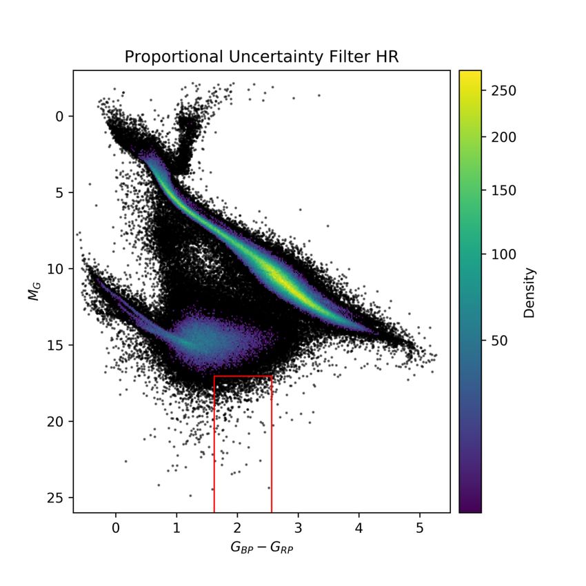
to conduct a realistic mirror star search with a more complete treatment of the SM nugget
in a future work. The methodology we develop in this paper to account for the wide range
of mirror star and hidden sector parameters can then be applied to this more realistic SM
calculation verbatim.
     Finally, we demonstrate how the non-observation of mirror stars can be used to set
constraints on the abundance and properties of mirror stars in our immediate stellar
neighborhood.1 In general, this depends on the mirror star mass distribution, which is
unknown and currently impossible to predict. Fortunately, this task can be simplified by
recognising that the most important feature of the mirror star distribution for the purpose
of setting constraints is just the mass of the lightest visible mirror stars. This focuses future

                                                                                                             JHEP07(2022)059
work on understanding the relationship between the fundamental Lagrangian of the dark
sector and the properties of “mirror red dwarfs”, i.e. the lightest mirror stars that can form
and (if the dark sector has nuclear forces) sustain dark nuclear fusion.
     Our work is highly complementary to other proposed mirror star searches using mi-
crolensing surveys [48] and gravitational waves [49], since it probes the size of dark photon
kinetic mixing and also provides information about the local mirror star density as opposed
to their distribution on galactic or even cosmological scales.
     This paper is structured as follows. In section 2 we briefly review how mirror stars
produce optical/IR signals. In section 3 we develop our methodology to search for mirror
stars in Gaia and other stellar catalogue data, and apply it by conducting a toy search
using the simplified treatment for their optical/IR emissions. Section 4 explains how we use
non-observation of mirror stars to place constraints on their abundance and properties. In
section 5 we discuss our results and place them in the context of other mirror star searches.

2       Mirror star properties

We assume that part of dark matter is composed of atomic dark matter, with dark protons
of mass mp0 (or, more generally, dark nuclei Ni0 of mass mNi0 ), dark electrons of mass
me0 , and dark QED with interaction strength αD . This is a simple but sufficient stand-in
for more complicated dark sectors in models like the Twin Higgs. Dark atoms will form
mirror stars in our galaxy if they can cool efficiently, though their abundance and spatial
distribution as a function of the atomic dark matter fraction and other parameters is not
known. If the dark sector also features an analogue of strong interactions, then mirror stars
will initiate dark nuclear fusion in their core to shine in dark photons for extended periods
of time, a phenomenon expected to be robust even for physical constants very different
from the SM [50].
     The crucial mechanism that leads to Mirror Stars having a detectable signature is the
fact that they generically capture Standard Model material from the interstellar medium
(ISM) [9, 10] if the dark and SM photons have kinetic mixing Fµν FDµν in the Lagrangian.
The interaction cross section between regular and mirror matter is proportional to 2 , since
    1
    Since the sensitivity depends mostly on the bolometric magnitude of mirror stars in SM photons, the
constraints we derive are robust with respect to the approximations made in the simplified emissions model
of the captured SM nugget.

                                                  –3–
mirror matter acquires a millicharge under the SM photon. Thus, particles charged under
mirror electromagnetism inherit a small interaction with particles charged under regular
electromagnetism. This allows for scattering of incoming hydrogen and helium atoms/nuclei
off the mirror stellar material, which can lead to capture and, over the course of the mirror
star’s lifetime, significant accumulation of regular matter in the mirror star’s core. 2 In this
section, we qualitatively review how SM matter is captured in mirror stars to form a SM
nugget, how this nugget is heated up via interactions with the mirror star core, and how it
radiates thermal and X-ray SM photons. For details, see the full discussion in [9, 10].
     There are two distinct capture mechanisms for the incoming SM material: mirror-
capture, which involves the 2 -suppressed scattering off mirror stellar nuclei; and self-capture,

                                                                                                                 JHEP07(2022)059
which involves the much more efficient scattering off already-captured SM matter. The total
mirror-capture rate will be proportional to the total number of targets (i.e. dark nuclei)
in the mirror star, while self capture is generally so efficient that it is bounded by the
geometric limit given by the physical size of the nugget. Gravitational focusing is taken
into account for both mechanisms.3
     It is important to be able to estimate the equilibrium temperature of the SM nugget,
since this affects the self-capture rate (because the temperature determines the virial size
of the nugget which in turn determines its geometric capture limit), and also because the
nugget temperature determines the amount and characteristic frequency of the emitted
radiation and hence its signature in Gaia data. In [9] we presented simple estimates for
the heating and cooling rate of the SM nugget composed of hydrogen and helium, which
allow one to solve for the equilibrium nugget temperature. These estimates are accurate
at the order-of-magnitude level but computationally much faster than the more careful
calculations presented in [10]. We use these simplified calculation to demonstrate our mirror
star search methodology, since this makes it easy to consider large samples of mirror stars
with widely varying properties and understand their signatures in generality.
     The SM nugget is very small compared to the mirror star. For Sun-like mirror stars,
nugget radii of O(103 km) are typical [9]. We therefore regard the nugget as being entirely
contained within the mirror star core. As a result, there are two main energy transfer
mechanisms from the mirror star to the SM nugget: 1) heating via collisions between mirror
nuclei and SM nuclei and 2) mirror X-ray conversion. Collisional heating proceeds via the
same interaction as mirror-capture — photon portal induced Rutherford scattering. X-ray
conversion refers to the fact that in the presence of both visible and mirror matter, a mirror
photon can elastically convert to a Standard Model photon via a Thomson-scattering-like
process. These converted photons will have energies characteristic of the Mirror Star’s core
   2
     Note that the reverse process is also expected to occur: see [51], where the accumulation of dark baryons
in white dwarfs is used to place constraints on the local density of atomic dark matter.
   3
     In [9, 10], the thermal motion of mirror nuclei was neglected in the computation of self-capture. Taking
this thermal motion into account may dramatically increase the mirror-capture rate [52, 53] and lead to
an earlier switch-over to geometric self-capture, which would significantly enhance the mirror star signal
for scenarios with low mirror-capture rates. Since capture in the most visible mirror star candidates is
already dominated by self-capture, this would not significantly change the boundaries of the mirror star
signal regions we derive in section 3, but it does make the constraints we derive for very small values of the
kinetic mixing  conservative.

                                                   –4–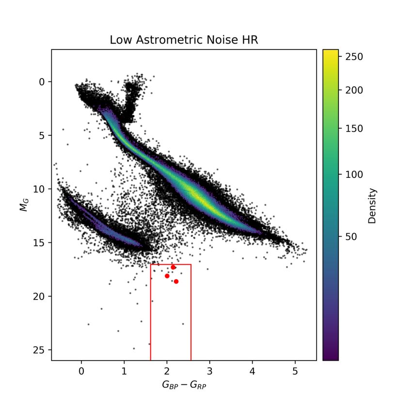
temperature, thus once converted can be a significant source of heating for X-ray opaque SM
nuggets. Some of these photons escape, and their detection in X-ray observations would also
provide a direct window into the mirror star’s interior, serving both as a smoking-gun signal
of the mirror star’s dark matter nature and a detailed probe of dark sector micro-physics.
     Cooling of the nugget, on the other hand, is very efficient (involving only Standard
Model processes), and tends to result in the nugget being significantly cooler than the core
temperature of the Mirror Star. Thus the nugget acts as a constant heat sink from the
Mirror Star core, drawing energy from the mirror stellar material which is then efficiently
radiated away in SM photons that pass through the mirror star material unobstructed.
(This has negligible effect on mirror star evolution for the range of their properties that

                                                                                                   JHEP07(2022)059
we consider.) In the emission models of [10, 10], the nugget temperature self-regulates to
O(104 K) because the free-free cooling process, being rapidly more efficient with increasing
ionization, is very inefficient below the ionization threshold. This model admits both
optically thick and optically thin solutions, with optically thick nuggets assumed to be
isothermal for simplicity.
     It is important to note that, since the internal structure, surface properties, and emitted
optical/IR spectrum of a nugget are determined by the physics of captured Standard Model
interstellar gas, the properties of the mirror star signal that we can observe are set in large
part by Standard Model physics. The observable properties of mirror stars will therefore be
robust over a wide range of mirror stellar physics parameters, allowing for telescope surveys
to probe wide regions of BSM parameter space.
     In a future work, we intend to address the details of SM nuggets’ hydrostatic structure
and thermal stability in the context of additional emission and absorption processes, such
as bound-free and bound-bound H− opacity and the collisionally-induced absorption of H2 ,
among others such as the effect of captured metals (see [54]). We anticipate that these
additional considerations will imply that the transition from optically thin to optically thick
nugget occurs at somewhat lower density than predicted in [10, 10], and that optically thick
SM nuggets are larger in radius and cooler in surface emission. The additional emission
processes may also shift the colour of optically thin nuggets.

3   Search for toy mirror stars

We now demonstrate how to conduct a search for mirror stars using Gaia and other public
stellar catalogue data. The main challenge is taking into account the wide range of possible
hidden sector micro-physics parameters, and their currently unknown relationship to the
detailed properties of the resulting mirror stars. Fortunately, since the optical/IR signals are
mostly determined by SM physics, mirror stars tend to show up in well-defined and distinct
regions of the Hertzsprung-Russell (HR) colour-magnitude diagram, which can be used to
define a mirror star search. We demonstrate this principle by developing a full mirror star
search pipeline using the simplified emissions model of [10], essentially conducting a particle
phenomenology-style BSM search over a large signal parameter space using astrophysics
data. This will make it straightforward to conduct a realistic mirror star search with a
more complete calculation of the SM nugget properties in the future.

                                             –5–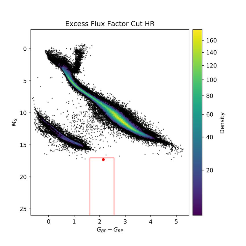
3.1   Defining a mirror star signal region
In principle, it would be possible to determine the range of allowed mirror star properties
from the atomic dark matter Lagrangian, but in practice, this is difficult and uncertain
in generality. It is more useful to parameterize mirror stars in terms of parameters that
directly determine their signature:

  • total mirror star mass MM S ,

  • radius rM S ,

                                                                                                 JHEP07(2022)059
  • core density ρcore ,

  • core temperature Tcore ,

  • age τM S ,

  • dark nucleus mass mN 0 . (If there are multiple dark nuclear species, we take this to be
    the average.)

The mass of the mirror electron, provided it is significantly less than the mirror nuclei,
does not affect our estimate for the signature. This simple mirror star model is sufficient to
estimate the optical/IR emission spectrum because (1) only the total number of targets
is needed to calculate mirror-capture, not their spatial distribution, and (2) the virial
radius SM nugget will generally be small relative to the size of the star, so we can estimate
the heating rate using only the temperature and density at the Mirror Star’s core. This
parameterization allows us to factorize the problem of understanding mirror star signatures
from the problem of understanding mirror stellar physics.
     To illustrate the various possible mirror star signals, we perform a scan by randomly
varying each of the above parameters on a log-scale by 2 orders of magnitude both above
and below their values for the sun, except for the constituent mass, which we vary by just
one order of magnitude above and below the mass of the proton, and the age, which we
require to be less than the age of the universe. We also vary the kinetic mixing parameter
and dark QED coupling  αD /αem in the range 10−10 − 10−13 . The output spectrum of
                            p

each mirror star’s SM nugget can then be convolved with the Gaia passband functions [55]
to compute its position in the Gaia HR diagram, assuming Gaia could measure the mirror
star’s parallax with sufficient accuracy to determine its absolute magnitude.
     The results of this scan are shown in figure 1, which is an HR-diagram in Gaia’s
passband magnitude coordinate space. The vertical axis is absolute magnitude, i.e. flux
measurement in the G (broad) passband, normalized via the parallax measurement. The
horizontal axis is the difference between the GBP (bluer) and GRP (redder) passbands,
indicating colour or temperature (bluer and hotter to the left). Each mirror star in our
sample corresponds to a dot in this plane. Horizontal contours indicate the mirror star
number density for a given absolute magnitude of its SM nugget that corresponds to 4
expected mirror star detections above Gaia’s relative magnitude threshold of 20. It therefore
corresponds to the mirror star number density that a non-observation at Gaia could exclude

                                            –6–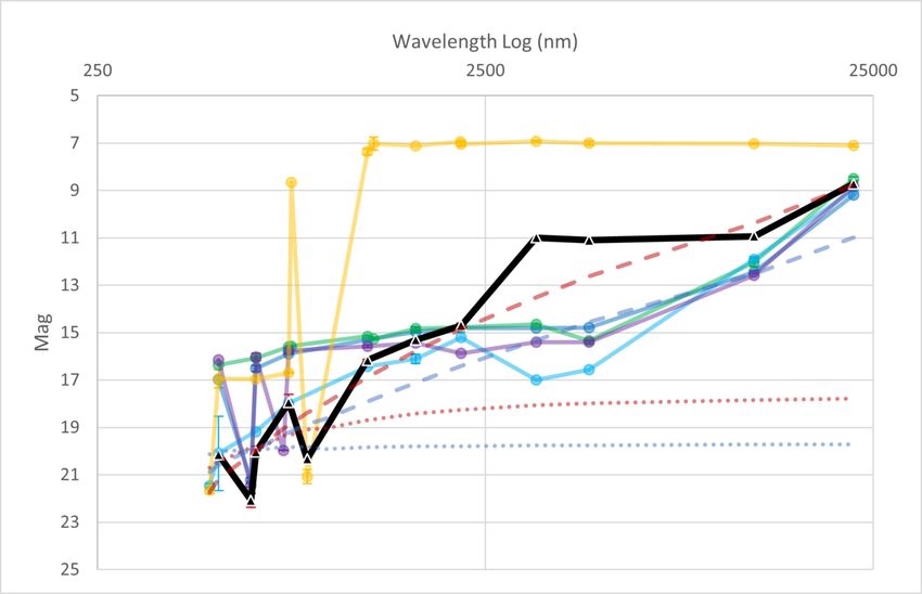
10

                                                                 104
                          15

                                                                 102

                          20
                                                                 100

                      G
                                                                      Mirror star
                          25                                                      -3
                                                                 10-2 density (pc )

                                                                 10-4
                          30

                                                                 10-6

                                                                                                        JHEP07(2022)059
                          35
                               -1   0   1        2      3    4
                                            GBP -GRP

Figure 1. Distribution of our simulated mirror star sample in Gaia’s HR diagram. Green dots:
10−10 ≤  ≤ 10−11 . Cyan dots: 10−11 ≤  ≤ 10−12 . Magenta dots: 10−12 ≤  ≤ 10−13 . The red box
is the signal region for our mirror star search in section 3. Horizontal contours indicate the mirror
star number density that corresponds to 4 expected mirror star observations in Gaia, corresponding
to the abundance that could be excluded by a non-observation in Gaia. The dashed black line
indicates the magnitude for which the maximum distance for detection is 100 pc.

at 95%-confidence-level. Of course, for a given mirror star mass, the mirror star number
density is already constrained just by measurements of the local DM mass density [56, 57].
We will discuss new constraints from Gaia in more detail in section 4.

     Figure 1 makes it clear that there are two distinct signal regions. These correspond
to the regimes in which the nugget of SM material is optically thin (“cooler” cluster of
points on the right) or optically thick (“hotter” cluster of points on the left). Our criteria
for making the optically thin/thick distinction is to compare the size of the nugget to the
path length of a photon with energies characteristic of the nugget’s average temperature.
Since the properties of the stars in our scan are varying wildly, and the interaction strength
between mirror and regular matter is also varying between several orders of magnitude, it
is natural to expect that the amount of captured material also varies dramatically. Thus
the photon mean free path can range from a small fraction of the nugget’s total size to
greater than the size of the star itself. Optically thin nuggets can cool more efficiently, since
any photon emitted throughout the nugget’s volume can escape; optically thick nuggets
cool only from their surface. This results in optically thick nuggets having a higher average
temperature than optically thin nuggets. As discussed above, a full calculation of the
optically thick nuggets’ properties is still outstanding and would have to take radiative and
convective heat transport into account. For the present analysis, we follow [9, 10] assume
it to be isothermal for simplicity. This may exaggerate the separation between optically
thick and thin nuggets in the HR diagram, but is sufficient for the purposes of this toy
demonstration study.

                                                       –7–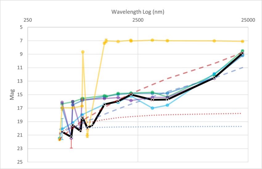
JHEP07(2022)059
Figure 2. These figures are the HR (top) and CC (bottom) diagrams for the GAIA data sets with
finer filter settings. On the left are sources selected with parallax and flux error filters; on the middle
are those selected by an additional astrometric noise cut; and on the right are those that survive an
additional excess flux cut. The predicted mirror star region is overlaid on top of HR diagram.

     Another feature that leads to the separation between these two regions on the HR
diagram is the fact that the spectral shape of an optically thin nugget is determined primarily
by the spectrum of emitted bremsstrahlung radiation, which is flat at low frequencies. On
the other hand, for optically thick nuggets low frequencies are more easily absorbed and
the spectrum approaches that of blackbody surface radiation. (This is also responsible
for the bunching of points to the left, as the difference between BP and RP passbands
approaches a constant for very hot blackbodies.) A more realistic nugget calculation will
include additional emission processes which may shift the colour of optically thin nuggets,
but this will likely preserve the separation from optically thick nuggets in the HR diagram.
     Of course the transition from optically thin to optically thick should be gradual during
the Mirror Star’s evolution, as more matter is accumulated and the nugget density increases.
However, by taking into account the full frequency and temperature-dependence of optical
depth, as well as the known accumulation rate and hence temperature evolution of the
nugget, we have verified that the crossover is very fast compared to the lifetime of the star,
so we are justified in not modelling the crossover in detail for our scans.
     In conclusion, our calculation shows that mirror stars are likely to show up in one of
two distinct regions of the HR diagram. This informs mirror searches using Gaia data.

3.2    Identifying mirror star candidates
Mirror stars with optically thin SM nuggets (“optically thin mirror stars” for short) live in a
region of the HR diagram that is very distinct from the areas where regular main sequence

                                                  –8–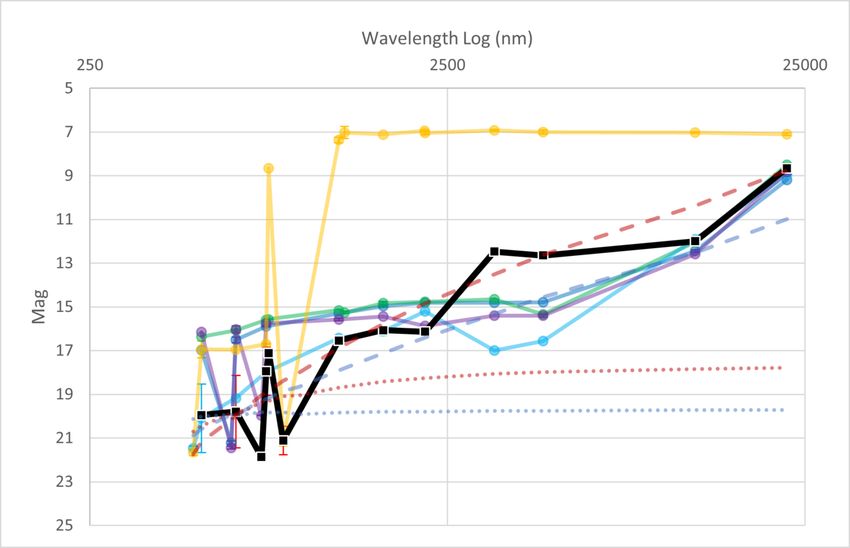
# Gaia DR2 ID           Parallax (mas) d (pc) RA (deg)    Dec (deg)    G (mag)    Bp (mag) Rp (mag)
 1   2930360704646411904 36.03829529   27.7   112.2433727 -19.29668099 19.519169 20.520412 18.375805
 2   4262452645550943232 46.46870759   21.5   285.8209665 -1.317245813 19.78358    19.94321   17.939726
 3   4506759318878397568 52.51774983   19.0   285.1298872 14.60245224   20.026243 20.152224 17.935917
 4   4061135605649798400 34.8478479    28.7   262.984546   -28.29006072 19.681303 19.908426 17.723442
 5   4064795192593397760 42.79213418   23.4   272.2102654 -26.22840704 19.602968 19.313232 17.277338
 6   4064883084836957568 38.80994358   25.8   271.6974055 -25.74928569 19.377226 19.568659 17.364256
 7   4077104186615316992 249.9741252   4.00   277.6285842 -24.70477356 20.593948 20.919155 18.541513
 8   4111242446355091200 26.786845     37.3   261.3680772 -24.37027144 20.256802 20.38141     18.364897
 9   4118771111750851328 53.17499257   18.8   267.41034    -20.84589839 19.128746 19.6124     17.486

                                                                                                          JHEP07(2022)059
 10 4118775406720100096 55.56323751    18.0   267.2904763 -20.76006312 19.296127 19.808765 17.800262
 11 4120764045300074240 170.5518763    5.86   267.0414042 -17.44704924 19.303873 19.32533     17.665956
 12 4314251119361223424 24.18581263    41.3   285.9615572 13.23008673   20.716675 21.419027 19.536842
 13 4514058083198280064 48.21504262    20.7   285.1280652 16.94445543   20.16315   20.768324 18.649843
 14 5928872365503657728 29.60234717    33.8   247.9725741 -55.47001062 20.517174 20.784586 18.449768

Table 1. This table contains the Gaia designation, parallax, right ascension, declination, g mag, bp
mag, and rp mag for each of the mirror star candidates. The first candidate (label in bold) is the
one we could further examine using other stellar databases.

stars and white dwarfs live. Furthermore, the visible/IR spectrum of these mirror stars
retains the shape of a typical bremsstrahlung spectrum, which is very flat at low frequencies
and should, in principle, be distinguishable from regular stars that more closely resemble
blackbodies. While the more complete calculation of optically thin mirror stars is likely to
add features like line emissions, the fact that an optically thin mirror star is distinguishable
from a black body or main sequence stellar spectrum is highly robust. Optically thin mirror
stars are therefore a natural first target, and we now describe a search for these objects in
the Gaia data release 2 [58]. A search for optically thick mirror stars requires more careful
treatment of the “white dwarf background”, and is left to future investigation.
     We define our optically thin search region as the red box in figure 13: 1.61 ≤ GBP −
GRP < 2.56 and absolute magnitude G > 17. This catches most of the mirror stars in
our random scan while staying away from the known locations of main sequence stars and
white dwarfs. Since we are searching for very dim objects with relatively large parallax,
we restrict our search to objects with distances smaller than 100 pc, for which distance
uncertainties are small.
     Following [59] we then apply some basic quality cuts to the Gaia
data,     requiring parallax_over_error,            phot_bp_mean_flux_over_error and
phot_rp_mean_flux_over_error all to be greater than 10, i.e., parallax and the
two (BP, RP) colour fluxes must be determined with better than 10% precision. The
resulting HR and colour-colour (CC) diagrams are shown in figure 2 (left), and is still
contain an unacceptably large contamination of sources intermediate between the main
sequence and the white dwarf tract, given that dust extinction within 100 pc is small. For
this reason we apply the astrometric_excess_noise < 1 cut. The suspect population is
significantly reduced, presumably because many binary and crowded or confused sources
are rejected [60]. The resulting HR and CC diagrams are shown in figure 2 (middle).

                                               –9–
JHEP07(2022)059
Figure 3. This plots shows all the passband functions used in our analysis, each normalized to
unity. Colour corresponds to different databases, while dashing distinguishes different passbands.
The vertical lines at the top indicate the transmisivity-weighted average of each passband, which
are used to assign a single frequency value for the flux of each passband in figure 6.
After performing this low astrometric noise cut, our optically thin mirror star signal
region contains 14 mirror star candidates, which we list in table 1. All of them would require
further analysis to determine whether they merit follow-up spectral or X-ray observations.
A reason for caution is that all of them have relative magnitudes near Gaia’s detection
threshold of 20, meaning they represent sources about as dim as Gaia can reliably see.
We now apply some further consistency checks on these candidates using Gaia data
as well as existing data from additional stellar catalogues. As we will see, only one of
them passes the strictest Gaia consistency check, although two others remain candidates
of interest.
Detailed spectral data are not commonly available for an arbitrary star in our galaxy,
although surveys such as SDSS and LAMOST provide increasing coverage [61, 62]. However,
various stellar catalogues contain absolute magnitude information over a range of wavelengths
as defined by their passband functions. If we can cross-match the mirror star candidates in
table 1 with objects detected in other surveys, we can assemble the magnitude information
from all the surveys’ passbands into a crude spectral measurement of the object over a range
of wavelengths. The catalogues we use, as well as their approximate wavelength ranges and
limiting magnitudes, where available, are the following.
• Gaia [1]: 300–1,100nm (MG < 18, MBP < 18, MRP < 18)
• Pan-STARRS [63]: 400–1100nm (Mg < 23.3, Mr < 23.2, Mi < 23.1, z < 22.3, y <
21.3)
• DENIS [64]: 700–2500nm (MI < 15.5, MJ < 14.5, MK < 13)
• ALLWISE [65]: 1000–2500nm (MW 1 < 17.1, MW 2 < 15.7, MW 3 < 11.5, MW 4 < 7.7)
• 2MASS [66]: 2500–30000nm (MJ < 15.8, MH < 15.1, MKs < 14.3)
We use the GATOR utility [67] to cross reference Gaia candidates with the other databases.
The passbands from all these surveys are shown in figure 3. We also indicate the
– 10 –JHEP07(2022)059
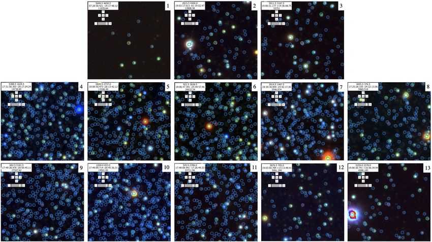
Figure 4. Pan-STARRS sky images of mirror star candidates 1–13, each marked with a red cross.
Blue and green circles indicate the known position of Gaia and 2MASS catalogue objects, respectively.
Only the first three candidates were detected by the other surveys. Candidate 14 is not in a region
of the sky imaged by Pan-STARRS. Each of these images is ∼ 1 arcmin in height and width.
λ (nm) Passband M1 M2 M3
486.645 PanS g
513.111 Gaia BP 20.520 19.943 20.152
621.463 PanS r 21.288 22.072
640.622 Gaia G 19.519 19.784 20.026
754.457 PanS i 20.413 21.870
777.732 Gaia RP 18.376 17.940 17.936
790.727 Denis I 18.478 17.114
867.950 PanS z 19.920 21.109 20.332
963.331 PanS y 19.549
1241.052 2mas J 16.463 16.542 16.162
1287.974 Denis J
1651.366 2mas H 15.985 16.06 15.307
2158.701 Denis K
2165.632 2mas Ks 15.003 16.132 14.69
3379.194 Wise W1 15.761 12.468 10.987
4629.297 Wise W2 15.723 12.646 11.101
12333.758 Wise W3 12.49 11.993 10.927
22253.236 Wise W4 8.84 8.651 8.714
Table 2. Absolute magnitudes M1,2,3 of our three mirror star candidates in the passbands of the
surveys we used. Blank fields indicate no data available.
– 11 –transmissivity-weighted average of each passband at the top of the plot, which we use to
assign each passband’s flux measurement a single wavelength value when assembling a crude
spectral energy distribution for each mirror star candidate.
In figure 4 we show Pan-STARRS sky images for the first 13 mirror star candidates.
Most of the candidates in table 1 were not detected in the DENIS, ALLWISE or 2MASS
catalogues. This is not surprising, as Gaia is significantly more sensitive. Only the first
three candidates show up in the majority of the other catalogues.
Some further insight might be gained by applying a final quality cut on the Gaia data.
Both blackbody and bremsstrahlung spectra of various temperatures should lie along the
JHEP07(2022)059
high-density line in the CC diagrams of figure 2. This can be easily understood, since
the RP and BP Gaia passbands measure complementary portions of the wavelength range
of the G passband, and their independent fluxes should approximmately sum to the G
flux. A strong deviation from the narrow region of consistency in the CC diagram could
indicate a measurement error of one or all of the passband magnitudes, or contamination of
the measurement by other sources close by in the sky. In fact, a visual inspection of the
Pan-STARRS images in figure 4 seems to suggest that all the candidates apart from #1
and #2 might suffer from source confusion, either due to identified nearby sources or due
to unidentified background sources.
The Gaia collaboration [59] suggests an excess flux factor cut to eliminate such
objects with potential errors in their colour measurement: 1 + 0.015 × (bp_rp)2 <
phot_bp_rp_excess_factor < 1.3 + 0.06 × (bp_rp)2 . After applying this cut, we are
left with the HR and CC diagrams in figure 2, and only our first mirror star candidate in
the optically thin signal region. This makes candidate #1 our primary mirror star candidate
for additional study, though we will also examine #2 and #3 since data in other catalogues
is available for them as well. The other candidates could still in principle be mirror stars,
and in a realistic analysis we should conduct follow-up analyses to see if they are present in
any other catalogues. However, for the purposes of demonstrating our search pipeline in
this toy analysis it is sufficient to focus on the first three and most high-quality candidates.
3.3 Examination of candidates #1, #2 and #3
For any mirror star candidate that is captured by multiple surveys, we can assemble a
pseudo-spectrum of magnitude measurements (λX , MX ) in the different passbands X, where
λX is the average wavelength of the passband with transmissivity PX (λ),
PX (λ)λdλ
R
λX = R , (3.1)
PX (λ)dλ
see figure 3. The magnitude MX in each passband is related to the flux density F (λ) (taken
to be the flux at 10pc) as follows [68, 69]:
Z λmax !
A
MX = −2.5 log10 dλ F (λ)PX (λ)λ + ZPX , (3.2)
109 hc λmin
– 12 –5
MG = 20
10
Mag
15 5000 K
10000 K
20
25
500 1000 5000 104
λ / nm
JHEP07(2022)059
Figure 5. Solid: predicted bremsstrahlung-like pseudo-spectrum of a mirror star with an optically
thin SM nugget at a temperature of 5000K (red) and 10000K (blue) in the simplified signal calculation
of [9]. Dashed: blackbody at same temperature for comparison. Each dot (λX , MX ) corresponds to
a survey passband X, see eqs. (3.1) and (3.2). All curves are normalized to an apparent magnitude
of 20 in Gaia’s G passband.
where λ is in nm, ZPX is the zero point4 of band X, and A is the telescope pupil area for
each survey.
Since optically thin mirror stars have a bremsstrahlung-like spectrum in our simplified
signal calculation, their pseudo-spectrum could be distinguishable from the expected
blackbody-like spectrum of regular stars. We demonstrate this in figure 5, where we
plot the predicted pseudo-spectrum for optically thin mirror stars and blackbodies at 5000K
and 10000K. The difference between the mirror-star prediction and the blackbody is much
greater than the variation due to the expected range of possible temperatures, with optically
thin mirror stars being comparatively much brighter at low frequencies. (The increase
at high wavelengths for the “flat” bremsstrahlung spectrum is due to the λ factor in the
integral of eq. (3.2).)
Pseudo spectra for mirror star candidates #1, #2, and #3 are shown in figure 6
(red diamonds, squares and triangles). These pseudo-spectra display the increase at high
wavelengths that might naively be suggestive of bremsstrahlung-like emissions. However,
it is not clear if the departure from the expected blackbody shape could be explained by
more benign astrophysics.
For guidance from the data, we randomly select 5 objects from the white dwarf region of
the Gaia HR diagram with observed temperatures in the range of 5000K — 9000K (marked
in HR diagram cutout in figure 6), and assemble their pseudo-spectra from the stellar
catalogues’ data in the same way as for the mirror star candidates. Their pseudo-spectra
are shown as the coloured dots in figure 6 (right), and look remarkably similar to our mirror
star candidates. Obviously, distinguishing mirror stars’ bremsstrahlung spectra from white
dwarfs using multi-band colours is not straightforward, since benign astrophysical effects
apparently give rise to a similar luminosity increase at long wavelengths as predicted for
4
In cases where the zero point for a given passband was not easily available, we derived it using the known
flux from Vega [70] and the fact that the observed magnitude of Vega is zero in any band by definition. For
passbands where the zero point was easily available, this agreed perfectly with the official values.
– 13 –JHEP07(2022)059
Figure 6. HR-diagram shows white dwarf region and mirror star candidates #1, #2, #3.
Also marked are 5 randomly selected comparison white dwarfs with temperatures from 5000K–
9000K. Plots show pseudo-spectra of mirror star candidates (black solid) and comparison white
dwarfs (coloured solid), using magnitude measurements in different stellar survey passbands. The
dashed/dotted opaque curves are the mirror star / blackbody theoretical expectations from figure 5
for comparison.
optically thin mirror stars. Reliably separating mirror stars from white dwarfs in this way
would likely require a more detailed analysis, but may be helped by additional emission
processes of the SM nugget that we have not included in our simplified signal calculation.
Given the comparison, it seems likely that these mirror star candidates are simply
particularly dim white dwarfs. In favour of this hypothesis, we note that their location
in the colour-magnitude diagram would be very close to the region populated by old and
massive helium-atmosphere white dwarfs [71] with a small amount of dust extinction.
Figure 7 demonstrates this possibility. However, their emission is also not inconsistent with
– 14 –5
H atm. 10.0
M He atm.
10 =0
age (Gyr)
.15
M 7.5
MG
M
=1
15 . 22
M 5.0
AV
=0
.5
2.5
20 2 13
0.0
−1 0 1 2
GBP − GRP (mag)
JHEP07(2022)059
Figure 7. Gaia colour-magnitude diagram comparing Candidates #1-#3 to model cooling sequences
of hydrogen-atmosphere and helium-atmosphere white dwarfs. The models plotted derive from [72–
74], and [75], combined and disseminated in [76]. Also shown is a reddening vector, corresponding
to 0.5 visual magnitudes of dust extinction as estimated by [61].
them being optically thin mirror stars in our emission model, and they are significantly
removed from the highly populated white dwarf region of the HR diagram. Follow-up
optical spectroscopy would be ideal to settle this issue.
4 Constraining mirror stars
Even if Gaia detects no mirror stars, it will still yield important constraints on the mirror
stars density. Figure 1 shows how each mirror star corresponds to a dot on the HR diagram,
and that non-detection can be translated into a 95% confidence level upper bound (4
expected but 0 observed signals) on the local number density of such mirror stars. In
this section, we show how to translate a non-detection by Gaia into constraints on mirror
star properties, like mass and core temperature. In principle, this might be connected to
fundamental parameters of the hidden sector Lagrangian in the future.
Note that our simplified model of mirror star emission may not be robust with respect
to the precise colour of the SM nuggets, but it is likely to give a good estimate of its
bolometric luminosity. We therefore derive these constraint projections without explicit
reference to any particular signal region in the HR diagram, since this may change with a
more sophisticated calculation. Rather, we simply assume that optically thin mirror stars
are distinctive and that a signal region can be defined within which non-mirror-stars can be
eliminated. This is justified given how different the emission mechanisms of optically thin
nuggets are compared to normal stars. The constraints on optically thin mirror stars are
therefore assumed to derive from a background-free search without any positive detection.
For optically thick mirror stars we consider two possibilities, one optimistic case where they
can be distinguished from regular stars, resulting in a zero-background-search, and one
pessimistic case where all white dwarfs count as backgrounds. Our results will therefore
give a good idea of Gaia’s sensitivity.
Even this effective approach, which does not start from hidden sector microphysics,
is extremely challenging in generality. Likelihood of observation depends not just on the
properties of a given mirror star, but also on their mass and age distribution in our stellar
– 15 –neighborhood. We therefore start with a non-physical warm-up by assuming that mirror
star properties and distributions are identical to SM stars. This teaches us which properties
of mirror star distributions most affect constraints, allowing us to use only the properties of
“mirror red dwarfs” to obtain simplified constraints on the mirror star density as a whole.
4.1 Warm-up: constraining a symmetric mirror sector
As a simple warm-up, we will assume that mirror-stars are perfectly SM-like, and that their
mass distribution is given by the IMF of SM stars given by [77]:
β
MM S
P (MM S ) ∝ (4.1)
JHEP07(2022)059
M
where
−0.3 when MM S /M < 0.08,
β= −1.3 when 0.08 ≤ MM S /M < 0.5, (4.2)
−2.3 when
0.5 ≤ MM S /M ,
and the various piece-wise parts are continuously joined and normalized to a given total
mirror star number density. Even if the mirror sector Lagrangian were an exact copy of
the SM, this scenario is not realistic, since in general the shape of the mirror star mass
distribution is influenced by the dynamics of mirror matter in our galaxy, which depends on
the fraction of dark matter that is mirror matter. However, for the purpose of illustration
we ignore this complication and assume that the mass function has a fixed shape with
only the normalization scaling directly with the local mirror star number density nM S , and
derive constraints on nM S as a function of αD /αem .
p
For different stellar masses above 0.14M , we use the MESA stellar evolution code [78–
82] to obtain the stars’ radius, core density, core temperature, and main sequence lifetime.
We then generate a large sample of mirror stars following the mass function, with each
star’s age chosen randomly from its lifetime. For a given αD /αem we can then compute
p
the bolometric magnitude in SM photons for each mirror star, and then compute the total
number of stars Gaia is expected to observe as a function of their number density:
Z Dmax
Nobs = nM S dD 4πD2 wi Θ (Gmax − mapp (mabs , D)) , (4.3)
X
0 i
where mapp is the apparent magnitude as a function of the absolute magnitude mabs and
the distance D, Gmax is the maximum magnitude we assume Gaia can see, Dmax = 100 pc
is the maximum assumed mirror star distance for reliable detection and parallax, and wi
are the relative weights assigned to each star according to their mass distribution, defined
such that i wi = 1. The sum is over mirror stars above Gaia’s detection threshold, since
P
the Heaviside function determines whether each star is visible at distance D. To obtain our
constraints we then find the value of nM S corresponding to a number of expected mirror star
observations Nobs that non-observation at Gaia can exclude, see below. Nobs is computed
separately for optically thin and thick mirror stars in our sample, and we take whichever of
the two resulting constraints on nM S is stronger.
– 16 –104
10
nMS / pc-3
10-2
10-5
10-13 10-12 10-11 10-10
1/2
ϵ (αD /α)
JHEP07(2022)059
Figure 8. Constraints on mirror star number density as a function of the kinetic mixing parameter
and dark QED coupling, assuming SM-like mirror stars with a SM-like mass function. For
10−11 ,
the dominant constraint comes from requiring the expected number of observed optically thin mirror
stars to be less than 4. For & 10−11 , the limit is dominated by optically thick mirror stars, with
the black (gray) curve corresponding to using current (optimistic future) limits on their observed
number. In the gray shaded region, the mirror star mass density excluded by Gaia exceeds the local
dark matter density. The black dotted line is the local number density of regular stars.
109
ϵ(αD /α)1/2 = 10-13
105
ϵ(αD /α)1/2 = 10-12
nMS / pc-3
10
ϵ(αD /α)1/2 = 10-11
10-3
ϵ(αD /α)1/2 = 10-10
10-7
0.1 0.5 1 5 10
MMS min / M⊙
Figure 9. Gaia constraints on SM-like mirror star number density, for β = −1 mass function with
minimum stellar mass MM S (dashed), or delta function mass distribution (solid). The coloured
curves correspond to four different values of the kinetic mixing parameter times dark coupling
constant. The shading indicates the effect of the unknown mirror star mass function. The more (less)
opaque curves correspond to the current (optimistic future) constraints derived from the optically
thick mirror stars. In the gray region, the mirror star mass density excluded by Gaia exceeds the
local dark matter density. The black dotted line is the local number density of regular stars.
Optically thin mirror stars live in a region of the HR diagram populated by very few
regular stars, so we set constraints assuming no signal has been observed with zero expected
background events. The limit nthin M S then corresponds to Nobs = 4 expected mirror star
observations. For optically thick mirror stars, a more sophisticated analysis would be
needed to obtain constraints that account for the “background” of regular white dwarf
stars. Such an analysis is beyond our scope, but we can still derive some constraints by
requiring that the total number of expected optically thick mirror stars does not exceed
– 17 –the number of observed white dwarfs in the Gaia dataset of our search, corresponding to
Nobs = NW D ≈ 1.36 × 10⁵ within 100 pc. This is extremely pessimistic but represents
an actual constraint of our analysis. Clearly, a realistic analysis could do much better,
but the best it could ever do in principle is perfect discrimination of white dwarfs from
mirror stars (e.g. via detailed spectral or X-ray measurements), in which case the search for
optically thick mirror stars becomes effectively background free and a projected constraint
can be set on nthick
M S by requiring Nobs = 4 expected observed events. We refer to these two
assumptions for optically thick mirror stars as the current and optimistic future constraints
respectively. Finally, we show combined constraints on (αD /α)1/2 from optically thin and
optically thick mirror stars in figure 8 by simply using whichever of the two constraints is
JHEP07(2022)059
stronger and requiring nM S < min(nthin M S , nM S ).
thick 5
In this example, the optically thick mirror star search would supply the strongest
current (optimistic future) constraint for αD /αem & 3 × 10⁻¹¹ (5 × 10⁻¹² ), while for
p
smaller kinetic mixings, the strongest constraint derives from the optically thin mirror
star search. This is reasonable, since for larger kinetic mixings, the interaction between
SM matter and the mirror matter is increased, leading to larger and hotter SM nuggets.
The current limits basically restrict the optically thick mirror star number density to be
smaller than the white dwarf number density, which is roughly an order of magnitude below
the total stellar number density (dotted horizontal line), while the optimistic assumption
for a possible future limit is about three orders of magnitude stronger, demonstrating the
sensitivity gain achievable with a dedicated mirror star observational search.
Let us now understand the importance of the mirror star mass distribution. Inspired by
the mass function of regular stars, we will make the simplified assumption that the mirror
star mass function follows a single power law:
β
MM S
P (MM S ) = A for min
M > MM S. (4.4)
M
The normalization constant A sets the total mirror star number density, while β is expected
to be a negative O(1) number that depends on mirror stellar physics and the dynamics of
atomic dark matter in our galaxy and stellar neighborhood. MM min is the minimum mass
S
of a mirror star that could be observable. This is a useful parameterization if the atomic
dark matter sector also contains an equivalent of dark nuclear physics, so that mirror
stars actually undergo energy conversion in their cores that drastically prolongs their main
sequence lifetime compared to the Kelvin-Helmholz time. In that case, in analogy to the
mass of the lightest red dwarf stars in the SM of ∼ 0.1M , there will be some minimum
mirror star mass that can initiate “dark fusion”.6
This simple mass function glosses over details at masses much larger than MM min (for
S
reasons that will be come obvious in a moment) and only has three parameters. The
normalization A is what we would like to constrain with observations. In theory, MM min
S
5
This simple combination is sufficient since the huge majority of mirror stars is either optically thin or
optically thick depending for low or high (αD /α)1/2 .
6
Depending on details of the dark sector, it is possible that “mirror brown dwarfs” contribute significantly
to the population of observable objects. We leave this possibility for future investigation.
– 18 –109
108
105
* * *
107
* * *
* * *
104
106
105 nMS109 10-6
10-4
10-5
10-6
108
* * *
105
107
* * *
* * *
104
106
105 10-6
103
MMS mN' MMS mN' MMS mN'
ϵ(αD /α)1/2 = 10-11 , = 0.1, = 0.1 ϵ(αD /α)1/2 = 10-11 , = 0.1, =1 ϵ(αD /α)1/2 = 10-11 , = 0.1, = 10
M⊙ mp M⊙ mp M⊙ mp
104 102
10-5
10-6 10-5 10-4
9
10 10-6 10-6
10-5
108 101
JHEP07(2022)059
10-5
* * 10-6
* 10-4
* * *
107 100
10-5
* * *
Tcore / K
nMS
106 pc-3
-1
10
105 nMS109
108
* * *
105
107
* * *
* * *
104
106
105
103
-4
10
MMS mN' MMS mN' MMS mN'
ϵ(αD /α)1/2 = 10-12 , = 0.1, = 0.1 ϵ(αD /α)1/2 = 10-12 , = 0.1, =1 ϵ(αD /α)1/2 = 10-12 , = 0.1, = 10
M⊙ mp M⊙ mp M⊙ mp
104 10-3
102
109 10-3
108 101
JHEP07(2022)059
* 10 -4
* *
* * *
107 * * * 100
Tcore / K
10-3 nMS
106 pc-3
-1
10
105
10-2
MMS mN' MMS mN' MMS mN'
ϵ(αD /α)1/2 = 10-12 , = 1, = 0.1 ϵ(αD /α)1/2 = 10-12 , = 1, =1 ϵ(αD /α)1/2 = 10-12 , = 1, = 10
M⊙ mp M⊙ mp M⊙ mp
104 10-2
109 10-5
10-3
10-3
108
*
*
*
*
*
* 10-4
107 *
10-5
* *
10-4
106 10-5
10-3
105
ϵ(αD /α)1/2 = 10-12 , MMS
= 10, mN'
= 0.1 ϵ(αD /α)1/2 = 10-12 , MMS
= 10, mN'
=1 ϵ(αD /α)1/2 = 10-12 , MMS
= 10, mN'
= 10
10-6
M⊙ mp M⊙ mp M⊙ mp
104 10-4 10-2
100 1000 104 105 106 107 100 1000 104 105 106 107 100 1000 104 105 106 107
ρcore / kg m-3
Figure 12. Same as figure 10 but for αD /αem = 10−12 .
p
4.2 Constraining mirror star abundance as a function of “mirror red dwarf”
properties
We now set constraints on the total local number density of mirror stars as a function of the
properties of “mirror red dwarfs”, i.e. their mass MM S ≡ MM min , radius, core temperature,
p S
nuclear constituent mass mN , and the mixing parameter αD /αem . As discussed above,
in the low-statistics limit the observation of mirror stars is entirely dominated by the most
common and lightest kind, justifying this enormous simplification.
To further reduce the dimensionality of the signal parameter space, we make the
additional assumption that mirror red dwarfs, like SM red dwarfs, have a much longer
lifetime than the current age of the universe. Therefore, the age of mirror stars today is
independent of their actual lifetime. While there is some dependence on the history of
mirror matter in our galaxy, we simplify our calculation by setting all mirror stars to have
the same representative lifetime (half the age of the universe), which should be a reasonable
approximation at our level of precision.
We also eliminate the mirror star radius as a free parameter by defining f = ρcore /ρavg ,
the ratio between the mirror star core and average density. For SM stars, f ∼ 1 − 300, so
– 21 –we fix f = 100 in our numerical analysis for simplicity, setting rM S as a function of MM S .
As we will show below, our final constraints on the mirror star density scale modestly with
√
this unknown ratio, nmax
MS ∼ f , meaning our constraints could be easily adapted to a given
understanding of mirror star physics which determines the true value of f .
It is now a straightforward exercise to repeat the analysis of the previous subsection
verbatim, for mirror red dwarfs with a given MM S , Tcore , ρcore and nuclear constituent mass
mN , assuming different kinetic mixings. The resulting Gaia bounds on the mirror star
number density for αD /αDM = 10−10 , 10−11 and 10−12 are shown in figures 10, 11 and 12
p
respectively. The coloured contours show maximum allowed nM S as a function of ρcore
and Tcore , for mirror red dwarf masses MM S = 0.1, 1, 10M (top to bottom) and nuclear
JHEP07(2022)059
constituent masses mN = 0.1, 1, 10mp (left to right). In each plot, to the left (right) of the
red line, constraints from the optically thin (thick) region provide the strongest constraint.
Above the green line, converted X-rays from the mirror star core contribute to heating the
SM nugget, changing the dependence of the nugget spectrum and magnitude on mirror star
parameters. The dashed magenta contours in the region where optically thick constraints
are dominant indicate the nM S bounds that could be achieved with a background-free
search, i.e. our optimistic future sensitivity projection in those parts of parameter space.
Finally, the three asterisks in each figure indicate ρcore , Tcore of a typical SM star with mass
0.2, 1, 10M (in order of increasing core temperature, as a reference. The constraints vary
widely, but at the order-of-magnitude level can be described reasonably well by an empirical
fit function to simple power laws. In the collisional heating-dominated optically thin region,
−3.33 −0.67 0.6 −1 !0.83
αD ρcore Tcore MM S mN
r
−3
nmax ∼ 10 pc .
MS
10−12 αem 10 kg m−3
5 107 K M mp
(4.5)
In the high-Tcore X-ray heating dominated region the bound is roughly
−3.33 −6.67 −1
αD ρcore Tcore MM S
r
−3
M S ∼ 350 pc
nmax . (4.6)
10−12 αem 103 kg m−3 108 K M
It is possible to understand these two sets of power laws from analytical estimates of
the capture and heating rate, using the expressions in [10]. Assuming that accumulation
quickly becomes self-capture dominated, the total number of SM nuclei in the nugget is
1/3 1/6
proportional to Cself ∼ vqesc R . vesc ∼
2 2 MM S /rM S ∼ MM S ρcore f −1/6 is the mirror star
p
escape velocity, and R ∼ Teq /ρcore is its virial radius, assuming an average equilibrium
√
nugget temperature Teq . The heating rate scales as dP/dV ∼ 2 αD nSM ρcore / mN Tcore for
nuclear scattering, and dP/dV ∼ 2 αD nSM Tcore
4 for X-ray heating, where nSM ∼ Cself /R3
is the number density of captured SM nuclei. The absolute nugget luminosity in the
optically thin case then scales as Labs ∼ R3 dP/dV , and the corresponding limit on the
−3/2
mirror star number density from Gaia scales as nmax M S ∼ Labs based on requiring less
than 4 predicted observations above Gaia’s apparent luminosity threshold. Putting all this
together, we find the following analytical expectation for the approximate scaling of the
– 22 –You can also read


