Estimating deer density and abundance using spatial mark-resight models with camera trap data - Oxford Academic
←
→
Page content transcription
If your browser does not render page correctly, please read the page content below
Journal of Mammalogy, 103(3):711–722, 2022
https://doi.org/10.1093/jmammal/gyac016
Published online March 8, 2022

Estimating deer density and abundance using spatial mark–resight
models with camera trap data
Andrew J. Bengsen,1,* , David M. Forsyth,1 Dave S. L. Ramsey,2 Matt Amos,3 Michael Brennan,3
Anthony R. Pople,3 Sebastien Comte,1 and Troy Crittle4
1
  NSW Department of Primary Industries, Vertebrate Pest Research Unit, 1447 Forest Road, Orange, NSW 2800, Australia
2
  Arthur Rylah Institute for Environmental Research, Department of Environment, Land, Water and Planning, 123 Brown Street,
Heidelberg, VIC 3084, Australia

                                                                                                                                                       Downloaded from https://academic.oup.com/jmammal/article/103/3/711/6544612 by guest on 27 June 2022
3
  Queensland Department of Agriculture and Fisheries, 41 Boggo Road, Dutton Park, QLD 4102, Australia
4
  NSW Department of Primary Industries, Biosecurity and Food Safety, 4 Marsden Park Road, Calala, NSW 2340, Australia
*To whom correspondence should be addressed: andrew.bengsen@dpi.nsw.gov.au

         Globally, many wild deer populations are actively studied or managed for conservation, hunting, or damage
         mitigation purposes. These studies require reliable estimates of population state parameters, such as density
         or abundance, with a level of precision that is fit for purpose. Such estimates can be difficult to attain for many
         populations that occur in situations that are poorly suited to common survey methods. We evaluated the utility of
         combining camera trap survey data, in which a small proportion of the sample is individually recognizable using
         natural markings, with spatial mark–resight (SMR) models to estimate deer density in a variety of situations. We
         surveyed 13 deer populations comprising four deer species (Cervus unicolor, C. timorensis, C. elaphus, Dama
         dama) at nine widely separated sites, and used Bayesian SMR models to estimate population densities and
         abundances. Twelve surveys provided sufficient data for analysis and seven produced density estimates with
         coefficients of variation (CVs) ≤ 0.25. Estimated densities ranged from 0.3 to 24.6 deer km−2. Camera trap
         surveys and SMR models provided a powerful and flexible approach for estimating deer densities in populations
         in which many detections were not individually identifiable, and they should provide useful density estimates
         under a wide range of conditions that are not amenable to more widely used methods. In the absence of specific
         local information on deer detectability and movement patterns, we recommend that at least 30 cameras be spaced
         at 500–1,000 m and set for 90 days. This approach could also be applied to large mammals other than deer.

         Key words:     abundance, capture–recapture, Cervidae, detection rate, fallow deer, population estimation, red deer, rusa deer, sambar deer

Reliable estimates of population size or density are needed                  cover in which the detection probability of methods such as
for wildlife research and management (Williams et al. 2002).                 terrestrial or aerial transects are typically too low to be useful
This is especially true for deer (family: Cervidae), which have              (Gardner et al. 2019).
a wide-ranging global distribution (Mattioli 2011) and are                      Spatial capture–recapture is a common approach to estimating
often subject to intensive population management such as con-                abundance and density from camera trap images (Efford and
trolled harvesting or culling (McShea et al. 1996; Hewitt 2011).             Fewster 2013; Royle et al. 2013). Spatial capture–recapture
A wide range of methods have been used to estimate deer abun-                methods require a large proportion of detected animals to be
dance (N) and density (D). The relative use of each method has               consistently identifiable as individuals by natural or anthropo-
varied regionally and temporally. Counts of deer or their sign               genic marks (Royle et al. 2013; Parsons et al. 2017). However,
from terrestrial or aerial transects have been most common in                capturing deer to apply markings such as ear tags or tracking
recent years (Forsyth et al. 2022). However, the use of camera               collars can be expensive, logistically challenging, and can com-
traps for deer surveys has increased since the 2000s, particu-               promise the health and survival of captured animals (Hampton
larly in North America (Forsyth et al. 2022). Camera trap sur-               et al. 2019; Bengsen et al. 2021). Capture and marking can also
veys are particularly well-suited to habitats with dense canopy              induce bias in estimators if the sample of marked animals is not

© The Author(s) 2022. Published by Oxford University Press on behalf of the American Society of Mammalogists.
This is an Open Access article distributed under the terms of the Creative Commons Attribution-NonCommercial License (https://creativecommons.
org/licenses/by-nc/4.0/), which permits non-commercial re-use, distribution, and reproduction in any medium, provided the original work is prop-
erly cited. For commercial re-use, please contact journals.permissions@oup.com

                                                                       711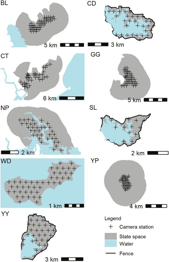
712                                                 JOURNAL OF MAMMALOGY

representative of the broader population of interest (Royle et al.   diverse real-world situations. Finally, we provide recommenda-
2013). Most deer species are characterized by a high proportion      tions for the use of SMR to estimate the abundance and density
of nondescript individuals and it is often the case that too few     of deer.
naturally marked and identifiable deer are detected for spatial
capture–recapture methods to be applicable (see below).
   Spatial mark–resight (SMR) models (Royle et al. 2013;                           Materials and Methods
Sollmann et al. 2013a) can overcome some of the above limi-             Camera trap surveys.—Deer species, topography, vegeta-
tations by combining detection information from a small pro-         tion, and site size varied among sites, but we used the same
portion of individually identifiable (i.e., “marked”) individuals    key principles to guide survey design throughout the study.
with information on unidentifiable (i.e., “unmarked”) individ-       We overlaid each of nine survey sites (Fig. 1) with a hexag-
uals. These models use the locations of detections from marked       onal grid and deployed a camera within a 50-m radius around
and unmarked animals to estimate the number and location of          the centroid of each grid cell. This provided an approximately

                                                                                                                                          Downloaded from https://academic.oup.com/jmammal/article/103/3/711/6544612 by guest on 27 June 2022
activity centers. Using this information, SMR models estimate        even spacing among neighboring cameras, while allowing us to
N within a defined state space that is usually larger than the       position cameras on game trails and other features that would
area that was surveyed (Chandler and Royle 2013; Royle et al.        enhance the probability of detecting deer that were using the
2013). SMR models and camera traps have been used to es-             area around the grid cell centroid. We avoided features such
timate carnivore population densities (e.g., Rich et al. 2014;       as ponds and large clearings that were not representative of, or
Kane et al. 2015; Forsyth et al. 2019) and have proven useful        pervasive throughout, the area close to the cell centroid. In this
for some ungulates (e.g., Jiménez et al. 2017; Gardner et al.        way, we sought to obtain a larger sample of individuals spread
2019). However, only one study has evaluated the applicability       across each study site than would have otherwise been pos-
of estimating N or D using camera traps with SMR methods for         sible, while minimizing bias in our estimates due to targeted or
any species of deer (Macaulay et al. 2019). That study showed        convenience sampling. The distance between centroids varied
that the approach was useful for estimating the density of one       among sites, ranging from 300 to 800 m. This spacing ensured
temperate deer species at a single site using an ad hoc sampling     that individual deer had the potential to be encountered at sev-
design. Further studies that apply a systematic and repeatable       eral camera locations, thereby creating spatial correlation in in-
sampling design to survey a range of species characterized by        dividual detection histories. We positioned a marker post 6 m in
different spatial and social behaviors and occupying a wider         front of the camera to delimit a standardized detection zone and
range habitat types are desirable for a more robust evaluation       only analyzed deer detections within that field of view. To avoid
of the method.                                                       the risk of modifying deer behavior and introducing an uncon-
   Estimates of N or D, termed N̂ or D̂, are subject to sampling     trolled source of bias to our estimates, no baits or lures were
error. The precision of estimates is often compared using the        used to attract animals to the camera. We used Reconyx HC600
coefficient of variation (CV), which is the ratio of the sample      cameras (Reconyx LLP, Holmen, Wisconsin) at all sites, un-
variability to the estimated value (Skalski et al. 2005). A CV of    less specified otherwise. Cameras were set horizontally on trees
≤0.25 is sometimes considered desirable for N̂ or D̂ (Skalski        or posts, aimed approximately 40 cm above ground level on
et al. 2005; 500–501), but the required CV will depend on the        the post 6 m from the camera. We set all cameras to record a
use of the estimates. A survey aiming to detect a small change       burst of five images in immediate succession for each camera
in N̂ or D̂, for example, will need greater precision than one       trigger event, with no mandatory elapsed time between subse-
aiming to detect a larger change. A recent review reported that      quent trigger events. We used a 2- to 3-month survey period at
most (72%) published deer abundance and density estimates            each site to strive for a sample size that would provide favor-
did not report precision, and only 26% of those that did re-         able precision and low bias. Simulation studies have suggested
ported a CV ≤ 0.25 (Forsyth et al. 2022).                            that survey durations of between 2 and 5 months should opti-
   In this paper, we report the application of SMR models to         mize precision and bias of spatial capture–recapture estimates
estimate D̂ from camera trap surveys of four deer species at         in species with intermediate life histories (DuPont et al. 2019).
nine sites in eastern Australia. Deer were deliberately intro-       Surveys at each site were timed to avoid seasons when spa-
duced into Australia to establish populations for hunting, but       tial behavior was likely to be unstable (e.g., rutting seasons for
some populations have established from escaped farm animals          fallow and red deer). None of the populations we surveyed were
(Moriarty 2004a). Knowing the abundance and density of wild          expected to experience intense seasonal mortality or movement
deer populations in Australia is important for management,           (e.g., due to hunting seasons or migration) that would violate
both as a hunting resource and to minimize their adverse im-         the assumption of population closure.
pacts (Moriarty 2004a; Davis et al. 2016). The sites at which           Study sites.—The nine study sites varied in their geographic
we conducted our study ranged from temperate to tropical and         characteristics, deer species present, and sampling intensity
from coastal to montane. The breadth of study area shapes,           (Table 1). Sites CD (145.41, −37.96), SL (145.31, −37.67), and
sizes, habitats, and deer species provide a powerful test of SMR     YY (145.15, −37.4) were water supply reservoirs in the hills
methods for estimating deer abundance and density. Our objec-        around Melbourne, Victoria. A large water body and a tall (ap-
tive was to evaluate the utility of SMR models for estimating D̂     proximately 2.4 m high) deer-resistant mesh fence provided
in deer populations and the levels of precision obtained under       hard inner and outer boundaries at these three sites (Fig. 2).
BENGSEN ET AL.—SPATIAL MARK–RESIGHT METHODS FOR DEER 713
These boundaries defined the state space and ensured geo-
graphic closure over the sampling area. The survey was con-
ducted during the 2017/2018 austral summer.
Sites GG (148.13, −36.04) and BL (148.32, −35.40) were lo-
cated inside Kosciuszko National Park in southeast New South
Wales. The state space was defined by a 3-km buffer around the
outer cameras, trimmed to exclude large expanses of treeless
farmland at both sites and a large water body at BL (Fig. 2).
These areas were excluded because they were not representa-
tive of the heavily wooded survey areas and did not provide
habitat that was likely to support activity range centers for
sambar or fallow deer. The buffer distance was selected to bal-
Downloaded from https://academic.oup.com/jmammal/article/103/3/711/6544612 by guest on 27 June 2022
ance computational speed and the requirement that deer with
activity centers beyond the state space would not appear on
the survey grid. Surveys were conducted during the 2018/2019
austral summer.
Sites YP (150.66, −23.39) and WD (149.87, −22.00) were
in coastal central Queensland and site NP (152.89, −27.24)
was a water supply reservoir in southeast Queensland. WD
was a small uninhabited island approximately 22 km from the
mainland. Deer populations at YP and WD were targeted for
eradication by local or state management agencies. A grid of
Swift 3C cameras (Outdoor Cameras Australia, Toowoomba,
Queensland, Australia) was used at each site. Cameras at YP
were deployed between May and August 2019 and those at
WD and NP were deployed between August and October
2019. The state space at YP was defined by a 3-km buffer
around the outer cameras, whereas the NP state space was
defined by a 1.5-km buffer which was trimmed to remove the
reservoir. The high tide mark provided a hard boundary at WD
(Fig. 2).
Site CT (152.67, −31.81) was a wetland reserve in coastal
New South Wales. The resident sambar deer population was
targeted for eradication by the local council. One rusa deer
was also photographed at one camera trap. Due to the two
species’ ability to hybridize (Martins et al. 2018) and diffi-
culties in consistently discriminating between them using
camera trap images, the single deer detection that was iden-
tified as rusa by antler morphology was included in the
sambar data set. A grid of 31 HS2X cameras (Reconyx LLP,
Holmen, Wisconsin) was deployed during the 2018/2019 aus-
tral summer. The state space was defined by a 3-km buffer
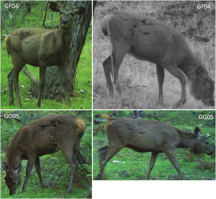
Fig. 1.—Location of nine study sites in the states of Queensland, New around the outer cameras, trimmed of open agricultural land
South Wales, and Victoria, eastern Australia. and human settlements (Fig. 2).
Table 1.—Site and survey characteristics for 13 deer density estimation surveys. Area is the area of the hexagonal grid used to site cameras at
sites with permeable boundaries or the area enclosed by fences or water for sites with impermeable boundaries (denoted by †).
Site Deer species Vegetation Terrain Cameras Area (km2) Days Camera spacing (m)
SL†
Red, Sambar Woodland Undulating 12 4.7 108 800
YY† Red, Sambar Woodland Undulating 29 14.6 109 800
CD† Fallow, Sambar Woodland Undulating 31 12.3 109 800
GG Fallow, Sambar Woodland, forest Montane 39 8.4 89 500
BL Sambar Woodland, forest Montane 40 8.7 89 500
CT Sambar Wetland, forest Flat 31 13.2 89 700
NP Rusa Woodland Undulating 35 7.6 58 500
YP Rusa Woodland Hilly 36 2.8 79 300
WD† Rusa Woodland, forest Undulating 44 3.8 64 300714 JOURNAL OF MAMMALOGY
we reduced the risk of failing to recognize subsequent recap-
tures. Such a failure would lead to the underestimation of de-
tection probability and overestimation of density (Evans and
Rittenhouse 2018). When assigning an initial identification,
observers considered whether markings were sufficiently ob-
vious that any trained observer would be able to recognize the
same individual at a different camera and time, including at
night under infrared illumination. Animals were not assigned
an individual identification code unless markings were clear
and obvious from multiple camera angles. Image brightness
and contrast were sometimes altered using Exifpro to enhance
the visual clarity of markings. Markings used for individual
Downloaded from https://academic.oup.com/jmammal/article/103/3/711/6544612 by guest on 27 June 2022
recognition included obvious antler shapes and deformations,
distinctive scarring on both sides of the body, and limb deform-
ations that were unlikely to greatly hinder mobility and intro-
duce bias into the estimation of movement patterns (Fig. 3). All
individuals at a given site were identified by a single experi-
enced observer.
We extracted metadata from camera trap images and con-
structed detection histories for the marked and unmarked com-
ponents of our samples using the camtrapR package (Niedballa
et al. 2016) in the R statistical computing environment (R Core
Team 2020). Detection histories for marked animals comprised
a three-dimensional array of each individual’s history of detec-
tion or nondetection at each camera station on each day. Many
deer showed markings that might enable them to be identified
as individuals in different sequences of images, but our con-
servative identification guidelines meant that fewer than 10
individuals were assigned at most sites. Unmarked detection
histories comprised a matrix of the number of detections at
each camera on each day.
Fig. 2.—Camera station and state space configuration at each of nine We fitted Bayesian SMR models using Metropolis-within-
deer survey sites. Gibbs MCMC algorithms (adapted from Chandler and Royle
2013; Royle et al. 2013; Sollmann et al. 2013a; Ramsey et al.
Density estimation.—The data used to estimate density in- 2015) implemented in R to estimate the density of each deer
cluded the camera trap spatial coordinates and spatial detection species present at each site. SMR models combine spatially
histories for recognizable (marked) individuals and unrecog- explicit observation models for marked and unmarked animals
nizable (unmarked) deer. We inspected camera trap images with a point process model that estimates the spatial distribution
and appended additional metadata using Exifpro (Kowalski of the activity centers of animals. In the observation models,
and Kowalski 2013). We grouped consecutive photos into the the probability of detecting an animal at a camera station is
same event if they were separated byBENGSEN ET AL.—SPATIAL MARK–RESIGHT METHODS FOR DEER 715
Downloaded from https://academic.oup.com/jmammal/article/103/3/711/6544612 by guest on 27 June 2022
Fig. 3.—Representative images of sambar deer S_GF04_001 taken from four occasions at two adjacent camera trap stations (GF04, GG05)
showing distinctive and consistently observable scarring on both sides of the body.
the marked individuals. The number of unmarked activity cen- prior (Γ(8.65, 30); x̄ = 0.29 km, SD = 0.10) on σ for sambar
ters is again estimated using DA. The process model assumes deer populations at sites BL and CT to overcome difficulties
that each animal’s spatial activity during a survey can be sum- with convergence. We based these weak priors on posterior
marized by a fixed, but unknown, number of activity centers distributions estimated from the same species at a similar site
contained within a defined area (the state space). The observed (GG; Supplementary Data SD2). We used between three and
and latent data are conditional on the number and location of six MCMC chains for each model. Convergence and burn-in
these unobserved activity centers. Activity center locations are adequacy were assessed by examining trace plots, overlap of
estimated as outcomes of a point process model within the state posterior distributions from each chain, and the Gelman–Rubin
space that includes the survey grid extended by a buffer be- statistic R̂ (Brooks and Gelman 1998). DA adequacy was as-
yond the grid that is large enough to avoid detections of animals sessed by visual checks for truncation in trace plots and poste-
with activity centers outside the state space. Thus, D̂ across the rior distributions. We used a series of short adaptation runs to
survey area is estimated from the number of activity centers in tune the candidate distributions for λ 0 and σ so that the accept-
the state space that is estimated using spatiotemporal variation ance rates for these parameters were between 0.16 and 0.42.
in detections of marked and unmarked animals (Chandler and MCMC autocorrelation was usually still large after tuning, so
Royle 2013; Royle et al. 2013). all chains comprised ≥85,000 draws after discarding burn-ins to
For each model, we estimated the decline in detection proba- attain effective sample sizes >1,000 for posterior distributions
bility with increasing distance from an animal’s activity center for population density. At sites with a permeable boundary,
using a hazard half-normal function. All spatial data were scaled we checked that the ratio of buffer size of the state space to σ
to kilometers and then centered to reduce autocorrelation and was >3 so that we could be confident that animals with activity
improve mixing in the Markov chain Monte Carlo (MCMC) centers beyond the state space were not detected (Royle et al.
chains. The shape of the hazard half-normal function is de- 2013). We used the mean of the posterior distribution for the
fined by the parameters λ 0 and σ, which estimate the expected point estimate for D̂ as posteriors were not heavily skewed.
number of detections per sampling occasion at an animal’s ac- To estimate the effects of variability in deer detections on
tivity center and the inflection point of the half-normal curve, precision, we used power functions to describe the effects of
respectively. We estimated a single λ 0 and σ for each combina- the number of unmarked detections, the number of marked in-
tion of site and species. In most cases, we used flat prior distri- dividuals, and the number of recaptures of marked individuals
butions for these parameters (λ 0, σ = U(0, 5)). We used a weak on the CV of the D̂ posterior mean: CV = aXb. A negative b716 JOURNAL OF MAMMALOGY
parameter would indicate that CV decreased with increasing maximum distance between detections for any individual was
values of the predictor variable. The three predictor variables 5,029 m for sambar and red deer at site YY. The mean distance
were all highly correlated (r ≥ 0.89), so we used a separate between detections of individual marked deer ranged from 193
model for each. Models were implemented in JAGS (Plummer m for sambar deer at CD to 1,249 m for sambar deer at BL.
2003) called via the runjags package (Denwood 2016) in R, Twelve of the 13 combinations of site and species provided
using three chains of 10,000 draws each after discarding 5,000 detection data that could be used in SMR models. There were
burn-in draws. insufficient detections of sambar deer at SL for modeling. On
To summarize the detection data, we estimated the expected three occasions, we were unable to obtain satisfactory MCMC
number of deer detections camera−1 day−1 using a Bayesian convergence after tuning and using weakly informative prior
negative binomial random effects model, specifying camera distributions. In these cases, we trimmed the detection histories
station and day as random effects. Detection rate data such as to include only the middle 21 days to reduce the risk of sam-
these have been often used as indices of relative abundance for pling over unstable activity ranges. We then reverted to using
Downloaded from https://academic.oup.com/jmammal/article/103/3/711/6544612 by guest on 27 June 2022
deer and other species and it is important to know how they flat priors (Table 2).
vary with D̂ (Parsons et al. 2017). For sambar deer, which was Estimated deer density ranged from 0.3 fallow deer km−2
the only species with more than three density estimates, we at GG (95% CrI = 0.1, 0.5) to 24.6 red deer km−2 at SL (95%
used linear regression to estimate the relationship between the CrI = 19.8, 30.6; Table 3). Estimated baseline encounter rates
summary index values (on their original log scale) and the pop- (λ 0) were 0.98.
Table 2.—Key data set and model characteristics used to estimate density of four deer species at nine sites. Nu is the number of deer detections
that could not be assigned to a recognizable individuals, Nm is the number of detections of recognizable individuals, and r is the number of indi-
vidual recaptures.
Deer species Site Camera Nu Nm r Mean group size SE group size Markov chain Monte Carlo σ prior
days used draws used (‘000s)
Fallow CD 3,141 141 4 14 1.37 0.55 1,470 U(0, 5)
Fallow GG 819 123 2 4 1.23 0.45 981 U(0, 5)
Red SL 1,198 309 20 61 2.55 0.88 1,458 U(0, 5)
Red YY 3,177 1,263 43 151 1.90 0.74 870 U(0, 5)
Rusa NP 735 68 4 11 1.28 0.55 1,470 U(0, 5)
Rusa WD 2,486 382 5 32 1.32 0.54 4,471 U(0, 5)
Rusa YP 756 68 3 7 1.47 0.63 1,171 U(0, 5)
Sambar BL 3,306 119 4 19 1.16 0.36 1,310 G(8.65, 30)
Sambar CD 3,141 587 8 20 1.35 0.50 834 U(0, 5)
Sambar CT 2,429 67 2 21 1.14 0.33 661 G(8.65, 30)
Sambar GG 3,268 186 8 42 1.23 0.54 1,111 U(0, 5)
Sambar SL 1,198 5 0 0 1.30 0.59 NA NA
Sambar YY 3,177 159 7 21 1.37 0.55 870 U(0, 5)BENGSEN ET AL.—SPATIAL MARK–RESIGHT METHODS FOR DEER 717
Table 3.—Population density posterior summary statistics for four deer species at nine sites.
Species Site Mean Mode 2.5% CrI 97.5% CrI CV
Sambar BL 0.73 0.64 0.33 1.35 0.36
Sambar CD 11.94 11.53 8.44 16.48 0.17
Sambar CT 0.48 0.41 0.24 0.84 0.32
Sambar GG 2.49 2.38 1.67 3.50 0.19
Sambar YY 3.93 3.56 2.53 6.29 0.25
Fallow CD 2.09 1.95 1.46 2.92 0.17
Fallow GG 0.29 0.25 0.12 0.53 0.36
Red SL 24.57 24.05 19.79 30.64 0.11
Red YY 19.76 19.64 17.58 22.17 0.06
Rusa NP 3.11 2.78 1.76 5.07 0.27
Rusa WD 10.34 9.93 7.84 13.32 0.13
Downloaded from https://academic.oup.com/jmammal/article/103/3/711/6544612 by guest on 27 June 2022
Rusa YP 0.68 0.42 0.21 1.77 0.61
CV = coefficient of variation, CrI = credible interval.
Fig. 5.—The detection rate index, calculated as ln(sambar detections
camera−1 day−1), increased with estimated population density (sambar
deer km−2). Solid lines represent 95% credible intervals of the esti-
mates and the dashed line and shaded polygon show the predicted
values and their 95% credible interval.
The diversity of study area shapes and sizes, environments (in-
cluding tropical and temperate, coastal and high-elevation),
deer populations, and camera grid characteristics in this study
provided a robust evaluation of the approach and highlighted
specific strengths and weaknesses that can be used to design
more effective surveys to estimate deer density and abundance.
Specific strengths of the methods used here included: (i) the
ability to estimate deer density in situations where more com-
Fig. 4.—Effects of increasing numbers of (a) marked individuals, monly used approaches such as transect-based animal counts
(b) recaptures of marked individuals, and (c) unmarked deer detections are unsuitable; (ii) the favorable level of precision attained in
on the precision (coefficient of variation [CV]) of population density most surveys; and (iii) the ability to incorporate prior informa-
estimates. Shading shows the 95% credible interval for each function. tion. We were able to estimate deer density in small, rugged,
and densely vegetated sites and in seemingly low-density or
Discussion cryptic populations that would be unlikely to provide sufficient
This study has shown that camera trap data in which few indi- numbers of detections for reliable estimation using transect-
viduals can be identified and recognized can be used with SMR based animal counts. This is important for informing intensive
models to estimate the population density of four deer species. management programs, such as eradication efforts, that often718 JOURNAL OF MAMMALOGY
target small geographic areas (e.g., sites CT, WD, YP) and between detections of individual sambar deer. A larger survey
low-density populations (e.g., Crouchley et al. 2011; Masters grid with greater spacing between cameras might have im-
et al. 2018). It is particularly valuable when target populations proved precision at this site, provided it could increase the
inhabit densely vegetated terrain that is difficult to survey using number of individuals captured without greatly reducing the
visual counts of animals, as is often the case for sambar deer number of spatial recaptures. However, greater camera spacing
(Leslie 2011). A global systematic review of over 5,000 deer may not have been beneficial for estimating density of rusa
abundance and density estimates concluded that mark–recap- deer at YP or fallow deer at GG. In both of these cases, deer
ture surveys using camera traps provided greater precision, detections were condensed within well-defined sections of the
on average (mean CV( D̂) = 0.39), than other survey methods survey grid and showed little spatial variation across the full
for which sufficient data were available (Forsyth et al. 2022). survey period. At YP, this was because the rusa deer population
Eleven of our 12 surveys provided greater precision than this was only recently established and did not appear to have spread
average, with seven surveys attaining CV( D̂) ≤ 0.25. A final widely, whereas fallow deer detections at GG were restricted
Downloaded from https://academic.oup.com/jmammal/article/103/3/711/6544612 by guest on 27 June 2022
specific advantage of the methods used here was the ability to to low elevations within the site. Increasing the camera spa-
produce and exploit prior information on spatial detections. cing at these sites would probably have led to a reduction in
Use of a weakly informative prior distribution on σ derived data available to estimate encounter rates and detection func-
from sambar deer detections at one site helped to achieve con- tions because fewer cameras would have been located in areas
vergence in survey models for sambar deer at two other sites, used by deer. Consequently, a greater camera spacing would
without the prior information dominating the posterior distri- probably have reduced the number of spatial recaptures without
bution. Prior information for σ can also be derived from te- increasing the number of detections of marked or unmarked
lemetry studies (e.g., Ramsey et al. 2015). The ability to use deer. In both cases, we trimmed the survey period to 21 days
prior information should be most valuable for surveys in which to reduce the risk that activity range centers were not stable
spatial recaptures are sparse, such as surveys of low-density during a long survey. This improved the mixing and stability of
populations or surveys in which camera spacing provides poor MCMC chains to an acceptable level. However, it also reduced
coverage of deer movements. the number of marked individuals, spatial recaptures, and un-
Our SMR models performed well in most analyses, requiring marked detections. Consequently, precision of the baseline en-
little adjustment beyond tuning the candidate distributions to counter rate and D̂ for rusa deer at YP were poor (CV λ 0 = 0.45,
achieve acceptance rates that optimized effective sample size CV D̂ = 0.61), compared to other surveys in this study.
and computation time. Density estimates were within the All but one of the 13 surveys in this study produced useful
range of expected values, given previous results from surveys results. However, the need for weak priors for two surveys and
of fallow deer (Bengsen et al. 2022), red deer (Amos et al. trimming of the survey period for three surveys highlights the
2014), and rusa deer (Moriarty 2004b) in Australia and sambar value of having an alternative method for estimating density
deer in their native range (Karanth and Sunquist 1992; Khan and abundance. Abundance indices based on detection rates
et al. 1996). Two cases (sambar deer at BL and CT) benefited have been criticized for their inability to determine the extent
from weakly informative priors on σ that improved MCMC to which changes in index value are attributable to variability
mixing, coverage, and posterior precision. In both cases, there in abundance or variability in detection probability (Anderson
was ≤10% overlap between the prior and the posterior distri- 2001; Sollmann et al. 2013b). Nonetheless, some camera-
bution, indicating that the data were sufficiently informative trapping studies have shown strong correlations between un-
to overcome the influence of the prior information (Gimenez gulate detection rates and densities estimated from the same
et al. 2009). The strong positive relationships between preci- data (Rovero and Marshall 2009; Parsons et al. 2017). The pos-
sion and increasing numbers of marked individuals, individual itive relationship between sambar deer detection rate and esti-
recaptures, and unmarked detections were consistent with ex- mated density in the present study suggests that the detection
pectations from previous simulation studies (Chandler and rate index used here could be useful for identifying the direc-
Royle 2013; Royle et al. 2013; Efford and Boulanger 2019), tion of coarse changes in population state over a wide range of
highlighting the importance of sample size for precision. densities (0.5 to 11.5 sambar deer km−2). Indices such as this
Three of the four cases in which models required additional are best suited to estimating changes in state when any differ-
adjustment to attain convergence or provided low precision ences in detection probabilities among surveys are likely to be
(CV > 0.35) had close camera spacing, relative to the observed heavily outweighed by differences in animal abundance, such
movement patterns of deer. Camera spacing for fallow deer as immediately before and after an intensive population control
at GG, rusa deer at YP, and sambar deer at BL was less than operation (Bengsen et al. 2014). Occupancy-based methods
σ, the detection function scale parameter. Simulation studies have also been popular for detecting differences among or
have shown that precision is often greatest at a camera spacing within populations using camera trap data (e.g., Parsons et al.
of 1.5σ to 2.5σ. Values in this range optimize the information 2017; Schlichting et al. 2020), but the requirement for spatial
available to estimate both the baseline encounter rate and the independence among survey stations in occupancy surveys
detection function by balancing the number of individuals cap- is inconsistent with the need for spatial dependence in SMR
tured, the number of recaptures, and the number and spatial surveys.
distribution of spatial recaptures (Sollmann et al. 2012; Efford Limitations.—The Bayesian SMR models used in this
and Fewster 2013; Royle et al. 2013). At BL, the close camera study provided a powerful and flexible tool for estimating
spacing relative to σ was due to the unusually long distances deer densities across a wide range of situations that were notBENGSEN ET AL.—SPATIAL MARK–RESIGHT METHODS FOR DEER 719
amenable to more commonly used methods such as transect- observed to bear markings without being conclusively identifi-
based counts of deer or their sign. However, effective use and able could be estimated and assigned using a probabilistic spa-
adaptation of these models requires a level of working knowl- tial submodel (Augustine et al. 2018; Whittington et al. 2018;
edge that can take a considerable commitment of time and ef- Murphy et al. 2019). However, the presence of natural mark-
fort to develop. Many wildlife managers wishing to use these ings that could not be used in the present surveys, such as ear
methods may need to partner with collaborators who already notches or scarring on a single flank, was often ambiguous.
have, or can acquire, the necessary expertise. Further, survey Recommendations.—Camera trap surveys for estimating
design constraints meant that the approach was best suited to deer density using SMR models should be designed to provide
situations in which the survey area was modest in size and re- data that can promote model convergence and produce a level
sults were not required urgently. The survey area constraint was of precision that is suitable for the aims of the study. In practice,
imposed by the need for camera spacing to be small enough to this will often mean maximizing precision, given a fixed level
provide spatial recaptures. The timeliness constraint was im- of survey effort. Our results showed that the numbers of marked
Downloaded from https://academic.oup.com/jmammal/article/103/3/711/6544612 by guest on 27 June 2022
posed by the long duration of surveys and the time taken to individuals, recaptures of marked individuals, and unmarked
process camera trap images and run models. detections were all important contributors to the precision of
Using the average σ estimate from our surveys of 0.54 km, density estimates. Based on our experiences and results across
a contiguous hexagonal survey grid comprising 33 camera sta- 12 combinations of site and deer species, we offer the following
tions could cover 33 km2 at a camera spacing of 2σ. This is general survey design and implementation recommendations
small, relative to the scale of 100s of km2 that can be covered which aim to improve the likelihood of models achieving con-
by aerial survey, for example (Forsyth et al. 2022). Hierarchical vergence and good precision under a wide range of conditions:
survey designs that use clusters of camera stations such that
spatial recaptures can occur within widely spaced groups of 1) Survey design should make full use of existing informa-
cameras could extend the spatial area sampled by survey grids tion on the likely spatial distribution, movement patterns,
(Efford and Fewster 2013; Sun et al. 2014). Optimization cri- and detection probabilities of the target species. Ideally,
teria and functions are available to help predict the most infor- such information would be derived from a local pilot
mative detector station layouts for a given survey area (Dupont study (Kristensen and Kovach 2018), but it could also be
et al. 2021). drawn from previous studies in other areas.
The time constraint could be reduced in some cases by short- 2) A 90-day survey period should often provide a balance
ening the survey duration. Three surveys produced results using of sample size, activity range stability, timeliness of re-
21-day survey periods, although precision was lower than all sults, and flexibility to subset the data. Our cameras were
but one of the other surveys which ranged from 64 to 109 days. deployed for between 64 and 109 days which provided
An optimal survey duration would be long enough to collect the opportunity to collect useful sample sizes. In three
and exploit as much detection data as possible while being cases, the full survey duration may have been too long to
short enough to maintain demographic and geographic popula- ensure population closure or stability of activity ranges.
tion closure (Royle et al. 2013). Processing many thousands of However, we were able to use a subset of data from the
camera trap images and carefully identifying individuals is also full survey period for analysis, whereas a survey cannot
time-consuming and expensive. Machine-learning algorithms usually be extended once the data have been collected and
are being developed to assist with identifying different species found to be insufficient.
and individuals in camera trap images (Schneider et al. 2019; 3) Surveys should be conducted during periods when spa-
Tabak et al. 2019; Meek et al. 2020). tial behavior is most likely to be stable. Long periods of
A further limitation of our surveys was the need to discard spatial stability provide the greatest opportunity for long
data from individuals that could be clearly identified on some surveys and favorable sample sizes without violating the
occasions, but whose markings were not sufficiently obvious assumptions that the population is geographically closed
to allow them to be identified with certainty every time that and activity range centers are stable. Many deer species
they were photographed. Including these detections as marked and populations experience predictable periods of spatial
individuals would have led to underestimation of detection instability such as rutting, migration, and birthing seasons
probability and overestimation of density, so they were counted (e.g., Perelberg et al. 2003; Sawyer et al. 2005; Ciuti et al.
as only unmarked detections. Including detections with am- 2006) that should be avoided. Birthing seasons should
biguous markings would also reduce repeatability due to in- also be avoided to avoid violating demographic closure,
consistencies among observers. This might have been partially as should periods of predictably high mortality, such as
overcome by using paired cameras that photographed both harsh winters or intense hunting seasons.
flanks of animals simultaneously (Karanth et al. 2011), al- 4) In the absence of site-specific prior information, a min-
though this would have increased deployment and processing imum of 30 cameras is desirable, but surveys should use
costs. White-flash cameras capable of recording greater in- as many cameras as practicable to ensure good spatial
formation content from detections in low light could also have coverage and sample size. All of our surveys that used at
been used, but this may have increased the risks of aversive re- least 29 camera stations achieved acceptable results. One
sponses from deer (Henrich et al. 2020) and theft of cameras by survey using 12 camera stations also achieved good re-
people. Alternatively, latent identities of detections that were sults in a small, insular site with a high-density red deer720 JOURNAL OF MAMMALOGY
population that provided a large sample size, despite the Steve Burke, Cameron Mulville, and Darrius Mann (Queensland
small effort. However, the same survey grid provided in- Parks and Wildlife Service) assisted with surveys at WD. Dave
sufficient data to estimate the density of a sparser sambar Mitchell, John Wyland, and Glenn McIntyre of Livingstone
deer population constrained within the same site. Shire Council assisted with surveys at YP. Jess Doman (SEQ
5) Camera spacing should reflect expected values of σ. Camera Water) assisted with site access at NP. Andrew Claridge (NSW
spacings of 1.5σ to 2σ are often considered desirable for DPI), Rena Gabarov, and Dave Caldwell (Wildlife Unlimited)
spatial capture–recapture studies (Efford and Boulanger assisted with surveys at BL and GG Anthony Marchment (Mid-
2019) and this should hold for SMR models. However, Coast Council) and Mark Lamb (Pest Lures) assisted with sur-
when detection probabilities are low, as was often the case veys at CT. Naomi Davis, Rena Gabarov, Molly Vardenega,
in our surveys (mean λ0 = 0.10 ± SD 0.17), a camera spacing and Sylvain Rouvier assisted with image processing and
< σ may provide greater precision (Kristensen and Kovach estimating interobserver agreement. We thank the three anon-
2018). For some species, ranges of expected values of σ can ymous reviewers for insight and comments that improved the
Downloaded from https://academic.oup.com/jmammal/article/103/3/711/6544612 by guest on 27 June 2022
often be estimated from telemetry data or from the results manuscript.
of the present study, although results from local camera trap
surveys will usually be preferable. Given the range of σ es-
timates from our surveys, a camera spacing between 500 Funding
and 1,000 m should often provide an optimal balance of Surveys at sites GG, CD and SL were funded by Melbourne
numbers of individuals and numbers of spatial recaptures. Water. Surveys at sites BL, GG and CT were funded by
Combinations of camera numbers and spacing that produce New South Wales Department of Primary Industries (Game
survey grid extents much smaller than the size of animal ac- Licensing Unit and Special Purpose Pest Management Rate).
tivity ranges cannot be expected to provide reliable results Surveys at NP, YP and WD were funded by the Queensland
(Sollmann et al. 2012; Efford and Boulanger 2019). Government’s Land Protection Fund.
6) Spatial clustering or irregular distribution of cameras
should be considered when the number of cameras and
suggested spacing are insufficient to cover the area of in- Supplementary Data
terest. We did not evaluate this in the present study, but Supplementary data are available at Journal of
sambar deer density estimation at site BL may have bene- Mammalogy online.
fited from this approach. Clustered survey designs can Supplementary Data SD1.—Density plots of time differ-
increase the area covered by a camera trap survey and the ences between successive camera triggers caused by four deer
number of individuals detected without biasing spatial species at nine sites.
capture–recapture parameter estimates (Sun et al. 2014; Supplementary Data SD2.—Posterior summary statistics
Efford and Boulanger 2019; Dupont et al. 2021). The op- for spatial mark–resight parameters.
timal allocation of effort across cluster size and number
of clusters can be explored using optimization algorithms
and simulations (Sun et al. 2014; Efford and Boulanger Literature Cited
2019; Dupont et al. 2021). Amos M., Baxter G., Finch N., Lisle A., Murray P. 2014. I just want
to count them! Considerations when choosing a deer population
monitoring method. Wildlife Biology 20:362–370.
Conclusion Anderson D.R. 2001. The need to get the basics right in wildlife field
Our study shows that SMR models can be used with camera studies. Wildlife Society Bulletin 29:1294–1297.
trap grids to estimate the density and abundance of deer. The Augustine B.C., Royle J.A., Kelly M.J., Satter C.B., Alonso R.S.,
Boydston E.E. Crooks K.R.. 2018. Spatial capture–recapture with
method provided precise and biologically plausible estimates
partial identity: an application to camera traps. The Annals of
of abundance for four deer species at most of the nine sites Applied Statistics 12:67–95.
we surveyed in eastern Australia. The diversity of deer spe- Bengsen A.J., Forsyth D.M., Ramsey D.S.L., Amos M., Brennan M.,
cies (two temperate, two tropical) and study areas suggests Pople A. 2021. AndrewBengsen/wild deer spatial mark-resight
that the method has wide application globally. The models are models and data. Zenodo. doi:10.5281/zenodo.4849263.
extremely flexible, accommodating populations in which all, Bengsen A.J., et al. 2022. AndrewBengsen/Helicopter-based-
some or no individuals are recognizable. In the absence of spe- shooting-of-deer_revised. Zenodo. doi:10.5281/zenodo.6070097.
cific local information on deer detectability and movement pat- Bengsen A.J., Hampton J.O., Comte S., Freney S., Forsyth D.M.
terns, and assuming similar detection rates as those estimated 2021. Evaluation of helicopter net-gunning to capture wild fallow
across our study sites and species, we recommend that at least deer (Dama dama). Wildlife Research 48:722–729.
30 cameras be spaced at 500–1,000 m and set for 90 days. Bengsen A.J., Robinson R., Chaffey C., Gavenlock J., Hornsby V.,
Hurst R., Fosdick M. 2014. Camera trap surveys to evaluate pest
animal control operations. Ecological Management & Restoration
Acknowledgments 15:97–100.
Brooks S.P., Gelman A. 1998. General methods for monitoring con-
Surveys at sites CD, SL, and YY were conducted by Melbourne vergence of iterative simulations. Journal of Computational and
Water, led by Tim Sanders with guidance from DMF and AJB. Graphical Statistics 7:434–455.BENGSEN ET AL.—SPATIAL MARK–RESIGHT METHODS FOR DEER 721
Chandler R.B., Royle J.A. 2013. Spatially explicit models for infer- Jiménez J., Higuero R., Charre-Medellin J.F., Acevedo P. 2017.
ence about density in unmarked or partially marked populations. Spatial mark-resight models to estimate feral pig population den-
The Annals of Applied Statistics 7:936–954. sity. Hystrix 28:208–213.
Ciuti S., Bongi P., Vassale S., Apollonio M. 2006. Influence of Kane M.D., Morin D.J., Kelly M.J. 2015. Potential for camera-traps
fawning on the spatial behaviour and habitat selection of female and spatial mark-resight models to improve monitoring of the crit-
fallow deer (Dama dama) during late pregnancy and early lacta- ically endangered West African lion (Panthera leo). Biodiversity
tion. Journal of Zoology 268:97–107. and Conservation 24:3527–3541.
Crouchley D., Nugent G., Edge K. 2011. Removal of red deer Karanth K.U., Nichols J.D., Kumar N.S. 2011. Estimating tiger abun-
(Cervus elaphus) from Anchor and Secretary Islands, Fiordland, dance from camera trap data: field surveys and analytical issues.
New Zealand. In: Veitch C.R., Clout M.N., Towns D.R., editors. In: O’Connell A.F., Nichols J.D., Karanth K.U., editors. Camera
Island invasives: eradication and management. IUCN, Gland, traps in animal ecology: methods and analyses. Springer, Tokyo;
Switzerland; p. 422–425. p. 97–117.
Davis N.E., Bennett A., Forsyth D.M., Bowman D.M.J.S., Karanth K.U., Sunquist M.E. 1992. Population structure, density and
Downloaded from https://academic.oup.com/jmammal/article/103/3/711/6544612 by guest on 27 June 2022
Lefroy E.C., Wood S.W., Woolnough A.P., West P., Hampton J.O., biomass of large herbivores in the tropical forests of Nagarahole,
Johnson C.N. 2016. A systematic review of the impacts and man- India. Journal of Tropical Ecology 8:21–35.
agement of introduced deer (family Cervidae) in Australia. Wildlife Khan J.A., Chellam R., Rodgers W.A., Johnsingh A.J.T. 1996.
Research 43:515–532. Ungulate densities and biomass in the tropical dry deciduous for-
Denwood M.J. 2016. runjags: an R package providing interface util- ests of Gir, Gujarat, India. Journal of Tropical Ecology 12:149–162.
ities, model templates, parallel computing methods and additional Kowalski M., Kowalski M. 2013. ExifPro photo browser v 2.1.0.
distributions for MCMC models in JAGS. Journal of Statistical http://www.exifpro.com/ accessed 28 September 2017.
Software 71:1–25. Kristensen T.V., Kovach A.I. 2018. Spatially explicit abundance es-
Dupont P., Milleret C., Gimenez O., Bischof R. 2019. Population clo- timation of a rare habitat specialist: implications for SECR study
sure and the bias-precision trade-off in spatial capture–recapture. design. Ecosphere 9:e02217.
Methods in Ecology and Evolution 10:661–672. Leslie D.M. 2011. Rusa unicolor (Artiodactyla: Cervidae).
Dupont G., Royle J.A., Nawaz M.A., Sutherland C. 2021. Optimal Mammalian Species 43:1–30.
sampling design for spatial capture-recapture. Ecology 102:e03262. Macaulay L.T., Sollmann R., Barrett R.H. 2019. Estimating deer
Efford M.G., Boulanger J. 2019. Fast evaluation of study designs populations using camera traps and natural marks. The Journal of
for spatially explicit capture–recapture. Methods in Ecology and Wildlife Management 84:301–310.
Evolution 10:1529–1535. Martins R.F., Schmidt A., Lenz D., Wilting A., Fickel J. 2018. Human-
Efford M.G., Fewster R.M. 2013. Estimating population size by spa- mediated introduction of introgressed deer across Wallace’s line:
tially explicit capture–recapture. Oikos 122:918–928. historical biogeography of Rusa unicolor and R. timorensis.
Evans M.J., Rittenhouse T.A. 2018. Evaluating spatially explicit den- Ecology and Evolution 8:1465–1479.
sity estimates of unmarked wildlife detected by remote cameras. Masters P., Markopoulos N., Florance B., Southgate R. 2018. The
Journal of Applied Ecology 55:2565–2574. eradication of fallow deer (Dama dama) and feral goats (Capra
Forsyth D.M., Comte S., Davis N.E., Bengsen A.J., Mysterud A., hircus) from Kangaroo Island, South Australia. Australasian
Côté S.D., Hewitt D.G., Morellet N. 2022. Methodology mat- Journal of Environmental Management 25:86–98.
ters when estimating deer abundance: a global systematic review Mattioli S. 2011. Family Cervidae (deer). In: Wilson D.,
and recommendations for improvements. Journal of Wildlife Mittermeier R., editors. Handbook of the mammals of the world.
Management (in press). Lynx Edicions, Barcelona, Spain; p. 350–443.
Forsyth D.M., Ramsey D.S., Woodford L.P. 2019. Estimating abun- McShea W.J., Underwood H.B., Rappole J.H. 1996. The science
dances, densities, and interspecific associations in a carnivore com- of overabundance: deer ecology and population management.
munity. Journal of Wildlife Management 83:1090–1102. Smithsonian Institution Press, Washington, District of Columbia,
Gardner P.C., Vaughan I.P., Liew L.P., Goossens B. 2019. Using USA.
natural marks in a spatially explicit capture-recapture framework Meek P.D., Ballard G., Falzon G., Williamson J., Milne H., Farrell R.,
to estimate preliminary population density of cryptic endan- Stover J., Mather-Zardain A.T., Bishop J.C., Cheung E.K.W. 2020.
gered wild cattle in Borneo. Global Ecology and Conservation Camera trapping technology and related advances: into the new
20:e00748. millennium. Australian Zoologist 40:392.
Gimenez O., Morgan B.J.T., Brooks S.P. 2009. Weak identifiability Moriarty A.J. 2004a. The liberation, distribution, abundance and man-
in models for mark-recapture-recovery data. In: Thomson D.L., agement of wild deer in Australia. Wildlife Research 31:291–299.
Cooch E.G., Conroy M.J. editors. Modeling demographic pro- Moriarty A.J. 2004b. Ecology and environmental impact of Javan
cesses in marked populations. Springer, Boston, Massachusetts, rusa deer (Cervus timorensis russa) in the Royal National Park.
USA; p. 1055–1067. Dissertation, University of Western Sydney, Penrith, Australia.
Hampton J.O., et al. 2019. A review of methods used to capture and Murphy S.M., Wilckens D.T., Augustine B.C., Peyton M.A.,
restrain introduced wild deer in Australia. Australian Mammalogy Harper G.C. 2019. Improving estimation of puma (Puma concolor)
41:1–11. population density: clustered camera-trapping, telemetry data, and
Henrich M., Niederlechner S., Kröschel M., Thoma S., Dormann C.F., generalized spatial mark-resight models. Scientific Reports 9:1–13.
Hartig F., Heurich M. 2020. The influence of camera trap flash type Niedballa J., Sollmann R., Courtiol A., Wilting A. 2016. camtrapR:
on the behavioural reactions and trapping rates of red deer and roe an R package for efficient camera trap data management. Methods
deer. Remote Sensing in Ecology and Conservation 6:399–410. in Ecology and Evolution 7:1457–1462.
Hewitt D.G. 2011. Biology and management of white-tailed deer. Parsons A.W., Forrester T., McShea W.J., Baker-Whatton M.C.,
CRC Press, Boca-Raton, Florida, USA. Millspaugh J.J., Kays R. 2017. Do occupancy or detection rates722 JOURNAL OF MAMMALOGY
from camera traps reflect deer density? Journal of Mammalogy re-identification from camera trap data. Methods in Ecology and
98:1547–1557. Evolution 10:461–470.
Perelberg A., Saltz D., Bar-David S., Dolev A., Yom-Tov Y. 2003. Sikes R.S., and The Animal Care and Use Committee of the American
Seasonal and circadian changes in the home ranges of reintro- Society of Mammalogists. 2016. 2016 Guidelines of the American
duced Persian fallow deer. The Journal of Wildlife Management Society of Mammalogists for the use of wild mammals in research
67:485–492. and education. Journal of Mammalogy 97:663–688.
Plummer M. 2003. JAGS: a program for analysis of Bayesian graph- Skalski J.R., Ryding K.E., Millspaugh J. 2005. Wildlife demography:
ical models using Gibbs sampling. In: Hornik K., Leisch F., analysis of sex, age, and count data. Elsevier Academic Press,
Zeileis A., editors. Proceedings of the 3rd International Workshop Burlington, Massachusetts, USA.
on Distributed Statistical Computing; 20–23 March 2003; Vienna, Sollmann R., Gardner B., Belant J.L. 2012. How does spatial study
Austria. Technische Universität Wien; p. 1–8. design influence density estimates from spatial capture-recapture
R Core Team. 2020. R: a language and environment for statistical models? PLoS One 7:e34575.
computing, Version 3.6.2. R Foundation for Statistical Computing, Sollmann R., Gardner B., Parsons A.W., Stocking J.J.,
Downloaded from https://academic.oup.com/jmammal/article/103/3/711/6544612 by guest on 27 June 2022
Vienna, Austria. www.R-project.org/. Accessed 17 January 2020. McClintock B.T., Simons T.R., Pollock K.H., O’Connell A.F.
Ramsey D.S.L., Caley P.A., Robley A. 2015. Estimating popula- 2013a. A spatial mark–resight model augmented with telemetry
tion density from presence–absence data using a spatially explicit data. Ecology 94:553–559.
model. The Journal of Wildlife Management 79:491–499. Sollmann R., Mohamed A., Samejima H., Wilting A. 2013b. Risky
Rich L.N., Kelly M.J., Sollmann R., Noss A.J., Maffei L., Arispe R.L., business or simple solution—relative abundance indices from
Paviolo A., De Angelo C.D., Di Blanco Y.E., Di Bitetti M.S. 2014. camera-trapping. Biological Conservation 159:405–412.
Comparing capture-recapture, mark-resight, and spatial mark- Sun C.C., Fuller A.K., Royle J.A. 2014. Trap configuration and spa-
resight models for estimating puma densities via camera traps. cing influences parameter estimates in spatial capture-recapture
Journal of Mammalogy 95:382–391. models. PLoS One 9:e88025.
Rovero F., Marshall A.R. 2009. Camera trapping photographic rate as Tabak M.A., Norouzzadeh M.S., Wolfson D.W., Sweeney S.J.,
an index of density in forest ungulates. Journal of Applied Ecology VerCauteren K.C., Snow N.P., Halseth J.M., Di Salvo P.A.,
46:1011–1017. Lewis J.S., White M.D. 2019. Machine learning to classify animal
Royle J.A., Chandler R.B., Sollmann R., Gardner B. 2013. Spatial species in camera trap images: applications in ecology. Methods in
capture-recapture. Academic Press, Waltham, Massachusetts, USA. Ecology and Evolution 10:585–590.
Sawyer H., Lindzey F., McWhirter D. 2005. Mule deer and prong- Whittington J., Hebblewhite M., Chandler R.B. 2018. Generalized
horn migration in western Wyoming. Wildlife Society Bulletin spatial mark–resight models with an application to grizzly bears.
33:1266–1273. Journal of Applied Ecology 55:157–168.
Schlichting P.E., Beasley J.C., Boughton R.K., Davis A.J., Williams B.K., Nichols J.D., Conroy M.J. 2002. Analysis and man-
Pepin K.M., Glow M.P., Snow N.P., Miller R.S., VerCauteren K.C., agement of animal populations: modeling, estimation, and decision
Lewis J.S. 2020. A rapid population assessment method for wild making. Academic Press, San Diego, California, USA.
pigs using baited cameras at 3 study sites. Wildlife Society Bulletin
44:372–382. Submitted 21 May 2021. Accepted 25 January 2022.
Schneider S., Taylor G.W., Linquist S., Kremer S.C. 2019. Past,
present and future approaches using computer vision for animal Associate Editor was Patrick Zollner.You can also read