How Snowfalls Affect the Operation of Taxi Fleets? A Case Study from Harbin, China
←
→
Page content transcription
If your browser does not render page correctly, please read the page content below
Hindawi
Journal of Advanced Transportation
Volume 2022, Article ID 3215435, 14 pages
https://doi.org/10.1155/2022/3215435

Research Article
How Snowfalls Affect the Operation of Taxi Fleets? A Case
Study from Harbin, China

          Binliang Li ,1 Haiming Cai ,2 and Dan Xiao                              2

          1
              Shenzhen Transportation Operation Command Center, Shenzhen 518040, China
          2
              School of Transportation Science and Engineering, Harbin Institute of Technology, Harbin 150006, China

          Correspondence should be addressed to Haiming Cai; haicai@dtu.dk

          Received 29 January 2022; Revised 17 February 2022; Accepted 25 February 2022; Published 20 March 2022

          Academic Editor: Qizhou Hu

          Copyright © 2022 Binliang Li et al. This is an open access article distributed under the Creative Commons Attribution License,
          which permits unrestricted use, distribution, and reproduction in any medium, provided the original work is properly cited.
          Taxi network plays an important role in urban passenger transportation. However, its operation is greatly affected by weather,
          especially by snowfalls in cold region. In this study, we focus on the persistent effect of snowfall on taxi operation and propose an
          autoregressive distribution lag model (ARDL) to quantitatively analyse it. To support our study, the taxi GPS trajectory data
          collected in Harbin, China, during 61 days from 1 November to 31 December in 2015 is analysed. First, the daily average order
          volume (DAOV) is acquired through data sampling and processing. Then, combined with the data of daily snowfall during the 61
          days, the ARDL model is constructed. The result shows that the snowfall has a lag effect on taxi operation and it lasts about 3 days.
          To better interpret the result, visualization of total 6 days before and after a heavy snowfall is conducted. The result also indicates
          that weekends have a positive effect on operation. These results are expected to assist us to better understand the effect of snowfall
          on taxi operation and provide some policy suggestions for local municipal and transportation management departments to ensure
          the normal operation of taxi networks.

1. Introduction                                                           as to decrease the level of service or operating revenue. In
                                                                          addition, extreme weather may have some significant in-
All kinds of public transportation in cities have their own               fluence on safety [17–20].
characteristics and are influenced by many factors, such as                    An obvious conclusion that can be drawn is that different
geographical, economic, social, or cultural factors [1]. The              weather conditions affect urban public transports in different
study of these factors can help us better understand the                  ways and to different degrees. Some of these meteorological
essence of transportation modes and residents’ travelling                 factors have been well studied, including rainfall [9, 17, 18, 21],
characteristics. Among these factors, weather is considered               snowfall [11], temperature [13], wind [22, 23], or combinations
to be one of the exogenous determinants [2]. Operations of                of some of these factors [1, 2, 10, 14]. However, no matter what
taxis, as an important mode of urban public transport                     kind of weather factor it is, adverse weather condition has a
without fixed operating schedule like buses, are more far-                 significant negative impact on taxi operation and service. From
reaching and widely affected by extreme weather.                           the perspective of residents, it brings inconvenience and
    Different from some studies on the influence of climate                 unsafety and affects their daily trips. From the perspective of
on transportation [3–6], the impact of weather on public                  transport service providers, it reduces the quality of transport
transport is usually short-term [1], which may affect resi-                services they provide and decreases their operating revenue [2].
dents’ travelling decisions and mode choices [7–10], leading              From the perspective of city administrators, adverse weather
to changes in travellers’ trip plans, modes, or routes.                   affects the normal production and living order and increases
Weather may also greatly affect the operation of public                    the financial burden. In view of this, it is of great significance to
transports [11–15], such as decreasing the availability and               study the influence mechanism and range of a certain weather
speed and increasing transit time and trip duration [16], so              factor on the taxi operation.
2                                                                                           Journal of Advanced Transportation

     In the study of these influence mechanisms, an inter-           point (DOP) of each trip are obtained. Then, based on this,
esting phenomenon is the time lag effect of weather on               an autoregressive distributed lag (ARDL) model is proposed
traffic. The so-called time lag effect refers to that, in a time       to study the lag effect of snowfalls on taxi operation. Some
series, the current value of the explained variable is not only     visualization methods are applied to help better understand
affected by the current value of explanatory variable, but also      the lag effect. The remainder of the paper is organized as
affected by one or more periods of lag of the explanatory            follows. Section 2 describes the study area, data sources, and
variable or the explained variable itself. This time lag effect is   methodology used in this study. The results of the lag effect
well studied in traffic volume prediction [24–26], travelling         are analysed, and visualization of taxi operation conditions is
time or speed [27], traffic safety [28–30], traffic behaviours          conducted in Section 3 and Section 4. Finally, conclusions
[31, 32], logistics [33], and so on. Among the various weather      and suggestions are presented in Section 5.
types, snowfall is recognized as the most significant one,
because it cannot dissipate quickly after it falls to the roads,    2. Materials and Methods
which leads to a sustained impact on traffic for hours to days
after the snowfall. Many models have been constructed to            2.1. Study Area. The case study is carried out in Harbin
explain this lag effect. Some of the outstanding works are as        (125°42′–130°10′E, 44°04′–46°40′N), China, which is located
follows: Thomas Nosal et al. [25] used regression models            on the Northeast Plain of China. It is the capital of Hei-
with autoregressive and moving average (ARMA) errors to             longjiang Province and consists of 9 districts and 9 counties,
investigate the direct impact and triggered effects of weather       covering 53100 square kilometres with a population of 9.952
variables on hourly and daily cycle counts in Montreal,             million. In this paper, the study area is focused on the
Ottawa, Vancouver, and Portland as well as on the Green             downtown area, including Nangang District, Daoli District,
Route in Quebec. In the study of Yannis and Karlaftis [28],         Daowai District, Xiangfang District, Songbei District, and
an integer autoregressive (INAR) model is used to estimate          Pingfang District, as shown in Figure 1. The study area
the effects of weather conditions on different traffic safety           covers 4187 square kilometres with a population of 5.4872
categories, and mean daily precipitation height along with its      million [35]. In 2015, the per capita GNP in Harbin was
lagged value (1 day) was proved to be the most consistently         59027 CNY [35]. The main public transit system in Harbin
significant and influential variable. Combining quantile              includes buses, taxis, and metro.
regression with distributed-lag nonlinear models, Zhan et al.            Harbin is one of the major cities in China with higher
[34] examined the nonlinear and lagged effects of hourly             latitude and lower temperature. Due to its temperate con-
precipitation and temperature on ambulance response time            tinental monsoon climate, Harbin has a long and cold
(ART) at the 50th and 90th percentiles and found that               winter, lasting for five months (from November to March).
marginal temperature and precipitation have different de-            Its snowfall period is mainly from November to January,
grees of lag effects on ART. Zhang et al. [35] proposed an           sometimes with heavy snow. The minimum temperature
impulse response function based on the vector autore-               during November and December 2015 can reach − 29°C (on
gression model to provide insight into the cross effects of the      December 25). Despite the Harbin metro has been put into
traffic parameters and their responses to weather conditions.         use in 2013, there was only one line with 18 stations in 2015,
     However, although many researchers have carried out            serving 158,600 passengers per day on average [35].
extensive studies on other aspects of taxis [36–43], very few       Therefore, the majority of public transportation trips mainly
studies have dealt with the time lag effect of snowfall on           relied on buses and taxis, especially with the reduction of
normal taxi operations. As an important component of                passengers’ tolerance of waiting buses due to the snowfall
urban transportation system, the service level of taxi needs to     and low temperature in winter, and taxis play an important
be paid enough attention, especially in snowy days, where           role in public transportation in Harbin. Therefore, Harbin is
people’s tolerance to low temperature is reduced and buses          a very typical and appropriate city to conduct research on the
become unreliable and unpunctual. At the same time, as a            time lag effect of snowfall on taxi operation.
means of aboveground transportation, the operation of taxis
is inevitably affected by snow, thus affecting the travel of
citizens and the income of taxi drivers. Therefore, it is of        2.2. Data Source. By 2015, all taxis in Harbin had been
great significance to study the time lag effect of snowfall on        equipped and put into use with GPS devices. These GPS
taxis, from the perspectives of improving the service level of      devices record taxi location every 30 seconds and play an
taxis and even the whole urban transportation system, fa-           important role in monitoring the taxi operation and en-
cilitating the daily travel of citizens, improving the income of    suring the safety of drivers and passengers in real time. This
taxi drivers, and giving advice of strengthening the urban          study collected the GPS trajectory data of more than 13000
road snow removal and deicing work to local municipal               anonymous taxis in Harbin from November 1 to December
department.                                                         31, 2015. The data contains the ID, GPSID, longitude, lat-
     In this paper, a large-scale study is presented by sampling    itude, speed, status (vacancy or occupied), and other in-
and analyzing GPS trajectory data collected from more than          formation of each taxi. Table 1 shows a sample of taxi
13000 taxis in Harbin, China, for two consecutive months.           trajectory data.
First, through data sampling and processing, the average                As Table 1 shows, “DEVID” is a number to distinguish
daily order volume within 61 days from 1 November to 31             anonymous taxis; “STATE” represents the status of taxis and
December in 2015 and the pick-up point (PUP) and drop-off            the different state codes corresponding to different status,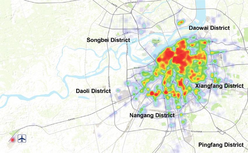
Journal of Advanced Transportation                                                                                                  3

                                             (a)                                        (b)

                        Figure 1: (a) Location of the study area and (b) the road network of the study area.

                                               Table 1: Taxi GPS data in Harbin city.
DEVID                  STATE              LATITUDE                 LONGTITUDE                 SPEED                 GPSTIME
0100324261               0                 45.708145                 126.59434                  0              2015/12/10 0 : 01 : 25
0300020062               0                 45.731396                 126.69875                  0              2015/12/10 0 : 01 : 24
0300061532               0                 45.72064                  126.67435                  0              2015/12/10 0 : 01 : 26
0100323182               1                 45.756107                 126.61123                 342             2015/12/10 0 : 01 : 37
0100304273               1                 45.75774                  126.58686                 176             2015/12/10 0 : 01 : 30
0300017510               1                 45.78798                 126.640755                  0              2015/12/10 0 : 01 : 28

such as “Vacancy” or “Occupied.” “LATITUDE” and                     2.3. Methodology
“LONGTITUDE” represent locations of taxis; “SPEED”
represents the instantaneous speed of taxis, and it is mea-         2.3.1. ARDL Model. In this study, an autoregressive dis-
sured in 100 meters per hour. “GPSTIME” represents the              tributed lag model was applied to study the lag effect of
real time of data.                                                  snowfalls on taxi operation. The ARDL model, originally
    Collection. Data of each day is stored in a single file, with    proposed by Charemz and Deadman to explain economic
18 to 28 million data items for each day. All the data sets have    phenomenon, has been widely used in various fields [44–48].
been cleaned by removing invalid points resulting from              Compared with the traditional cointegration test method,
device failure or recording errors. In this study, GPS tra-         the ARDL model has the following advantages:
jectory data of 25% of taxis were sampled as the research               (1) The ARDL method does not need to check in ad-
object, which accounts to 4 to 7 million items in one day.                  vance whether the time series has first-order single
Theoretically speaking, the 30-second sampling rate and                     integrity
such a large amount of GPS data can basically cover most of
the road network in the Harbin downtown. Figure 2 shows                 (2) The ARDL process of boundary test is robust enough
the trajectory of 3000 taxis, from which the basic outline of               to small samples, and the sample length needs to be
Harbin road network structure is depicted.                                  low
    From these data, the complete driving trajectory of each            (3) When the explanatory variable is endogenous, the
taxi in the sample in a day can be extracted. The meanings                  ARDL method can still get unbiased and effective
represented by different state codes are recognized in the                   estimates
study first. Figure 3 depicts a piece of driving trajectory of a
                                                                        (4) The ARDL method overcomes many problems
taxi. It denotes that the taxi cruises on the road in search of
                                                                            caused by nonstationary time series data, such as
potential passengers (in vacant status); then the driver picks
                                                                            false regression
up passengers at pick-up point (PUP) and starts to deliver
passengers to their destinations (in occupied status); after            Considering the above advantages of the ARDL model,
the passengers get off the taxi at drop-off point (DOP), the          this paper uses the ARDL model to study the impact of
taxi cruises on the road again to search for another potential      snowfalls on taxi operation, which is rarely applied to this
passengers (in vacant status again). Based on the cleaned           topic before.
data, all the PUPs and DOPs of the taxi sample in the city              The ARDL model is a branch of the distributed lag (DL)
every day can be extracted, and each PUP corresponds to a           model. If the current value Y(t) of the explained variable Y
specific DOP, which together denote a complete trip. Thus,           not only is affected by the current value X(t) of the ex-
some other parameters, such as daily average order volume           planatory variable X, but also obviously depends on the lag
(DAOV), can be calculated to support the follow-up study.           value X(t − 1), X(t − 2), such a model is a distributed lag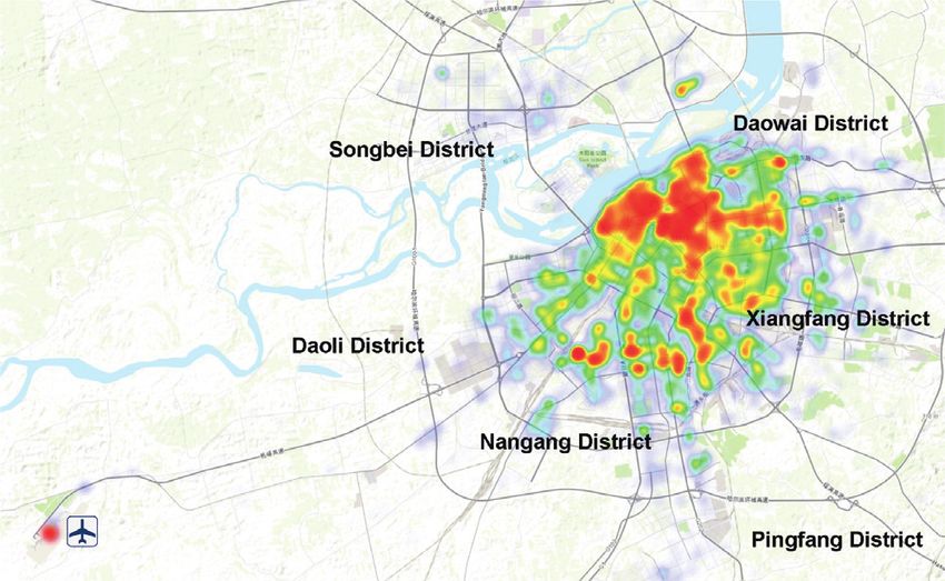
4                                                                                                Journal of Advanced Transportation

                                                                      number of parameters by imposing restrictions on the
                                                                      distribution of values that the ci coefficients could take.
                                                                          The assumptions for ARDL model are as follows:
                                                                          (1) The primary requirement of ARDL model is the
                                                                              absence of autocorrelation. It is required that the
                                                                              error terms have no autocorrelation with each other.
                                                                          (2) The time series data should follow normal
                                                                              distribution.
                                                                          (3) Any heteroscedasticity should not occur in the data.
                                                                              And the mean and variance should be constant
                                                                              throughout the ARDL model.
Figure 2: A one-day trajectory map of a sample of 3000 taxis within
the study area.                                                           (4) The time series data should have stationary either on
                                                                              I (0) or I (1), or on both. In addition, the model
                                                                              cannot run if any of the variable in the data has
                                                                              stationary at I (2).
                                                                          In this study, the daily snowfalls were taken as the ex-
                                              pick-up point           planatory variable. Considering that the number of taxis
                                                                      operating every day is variable and taxi drivers pay more
               drop-off point                                         attention to their income, which is positively correlated with
                                                                      the number of orders served by drivers, the study took the
                                                                      daily average orders volume as the explained variable of the
                                                                      model.
                                                    Occupied
                                                    Vacancy
                                                                      2.3.2. Granger Causality Test. Granger Causality Test was
      Figure 3: A piece of continuous trajectory of a taxi.           proposed by Granger, a famous econometric economist in
                                                                      California in 1969, and further developed by Hendry and
model. The term “autoregressive” indicates that along with            Richard. In the case of time series, the causal relationship
getting explained by the current value and the lag value of           between two economic variables X and Y can be defined as
X(t), Y(t) also gets explained by its own lag value(s), such as       follows: if the past information of variables X and Y is
Y(t − 1). Considering the autoregressive modelling of traffic           known, the prediction effect of Y is better than that of Y only
parameters mentioned in some previous studies [25, 49–51],            based on the past information of Y. That is, variable X helps
the lag of Y(t) was also considered in this study. Equation of        to explain the future change of variable Y, then variable X
ARDL (m, n) is as follows:                                            causes the change of variable Y, and there is causal rela-
                                                                      tionship between them. For two given time series X and Y in
Y(t) � α + β1 Y(t − 1) + · · · · · · + βm Y(t − m) + c0 X(t)          the period of t � 1, . . ., T, to test whether X is the cause of Y,
                                                               (1)
        + c1 X(t − 1) + · · · · · · + cn X(t − n) + εt .              two models can be constructed: one is as (1) shows, and the
                                                                      other is as follows:
    Here, m and n are the number of lags of Y and X, re-
spectively, βi is the coefficient for the explained variable Y            Y(t) � α + β1 Y(t − 1) + · · · · · · + βm Y(t − m) + εt .      (2)
and its lags, and cj is the coefficient for the explanatory
variable X and its lags, which is called lag weights, and they             If cj � 0 holds for all j � 1, 2, . . ., n, then variable X will
collectively comprise the lag distribution. They define the            not cause the change of variable Y, which does not constitute
pattern of how X affects Y over time. εt is a random dis-              a causal relationship, and the choice of lag period can be
turbance term.                                                        arbitrary. So we can assume H0 : cj � 0, j � 1, 2, . . ., n. Then,
    Given the presence of lagged values of the dependent              we regress (1) and (2) to obtain EES1 and EES2 of the ex-
variable as regressors, OLS estimation of an ARDL model               planatory square and RSS1 of the residual square and
will yield biased coefficient estimates. If the disturbance term        construct the following statistics: F � [(EES1 − EES2 )/
εt is autocorrelated, the OLS will also be an inconsistent            m]/[RSS1 /(T − (m + n + 1))]. F obeys the distribution that
estimator, and in this case Instrumental Variables Estima-            the first degree of freedom is m and the second degree of
tion was generally used.                                              freedom is T-(m + n + 1). Given the significance level a, there
    The distributed lag (DL (q), or ARDL (0, q)) models were          is a corresponding critical value Fa . If F > Fa , then reject the
widely used in the 1960 s and 1970 s. To avoid the adverse            hypothesis of H0 with the confidence of (1 − a). In the sense
effects of the multicollinearity associated with including             of Granger, X is the cause of Y. Otherwise, accept H0 ; that is,
many lags of X as regressors, it was common to reduce the             the change of Y cannot be attributed to the change of X.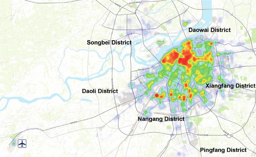
Journal of Advanced Transportation                                                                                                                                          5

3. Results                                                                           40
                                                                                                                                                                   6
3.1. Statistics of DAOV and Snowfall over 61 Days.                                   30

                                                                      orders (day)
Figure 4 shows the change of daily average order volume and
                                                                                                                                                                   4

                                                                                                                                                                       mm
snowfalls in 61 days. From the figure, we can see that the                            20
DAOV is obviously affected by the snowfalls, and the
                                                                                                                                                                   2
snowfalls still have a continuous impact on the following 2-3                        10
days. In addition, the daily average order volume of every
weekend has an increasement in different degrees compared                             0                                                                             0

                                                                                             Nov.7

                                                                                                     Nov.14

                                                                                                              Nov.21

                                                                                                                       Nov.28

                                                                                                                                Dec.4

                                                                                                                                        Dec.11

                                                                                                                                                 Dec.18

                                                                                                                                                          Dec.25
with the working days.

                                                                                                                          Date
3.2. ARDL Model Analysis. To use the autoregressive dis-
tribution lag model to study the time lag effect of snowfalls                                    Daily average order volumn
on taxi operation, a unit root test is implemented first to                                      weekends
check whether there is a unit root in the series of daily                                       Snowfall
average order volume and daily snowfall. When there is unit
root in the time series, it is regarded as nonstationary, which            Figure 4: Plot of the DAOV and snowfall over 61 days.
will lead to the existence of pseudoregression in regression
analysis. In this study, the Augmented Dickey-Fuller test
(ADF test) was used to perform the unit root test for the
stationarity of each series. The original hypothesis of the test                            Table 2: Results of the unit root test.
is that the time series of the daily average order volume and
snowfalls are both nonstationary. Table 2 shows the results of                    Test       Critical value
                                                                                             ADF                 p
                                                                                                                     Conclusion
unit root test for the two series.                                               form    1%  value 5%      10% value
     In the results, Y represents the explained variable, the      Y (C, 0, 1) − 4.331 − 3.546 − 2.912 − 2.594 0.001 Stationary
daily average order volume; X is the explanatory variable,         X (C, 0, 0) − 5.158 − 3.544 − 2.911 − 2.593 0.000 Stationary
which is snowfalls (in mm). In the test form (C, T, K), C, T,
and K represent constant term, trend term, and the order of
difference, respectively.                                                                  Table 3: Results of Granger Causality Test.
     As shown in Table 2, both the explained variable Y and
the explained variable X reject the original hypothesis at the          Original hypothesis: X is not the Granger cause of Y
significance level of 1%; that is, the time series of the daily     Lag order                    F-value                    p value
average order volume and snowfalls are both stationary             1                             10.922                     0.002
series; then, the Granger Causality Test can be implemented.       2                              4.004                     0.024
     According to the theory of Granger Causality Test, when       3                              2.853                     0.046
the snowfall X explains the average daily order volume Y           4                              2.408                     0.062
better than the average daily order volume Y explained solely      5                              2.587                     0.039
                                                                   6                              2.402                     0.044
by the lag term of itself, the variable X can be considered as
                                                                   7                              1.696                     0.139
the Granger cause of variable Y. The original hypothesis of
the test is that snowfall X is not the Granger cause of daily
average order volume Y. Table 3 shows the results of Granger           According to the results of Granger Causality Test, the
Causality Test under different lag orders of snowfalls.             paper sets the maximum lag order of the model as 6 and
     As shown in Table 3, when the lag order is 1 to 6, the        determines the model as ARDL (1, 3) according to AIC
original hypothesis is rejected at the significance level of 5%     criterion. Under BIC, HQC, and Adj. R2 criteria, the form of
(in which, when the lag order is 1, it is rejected at the          lag model is basically the same. Therefore, the model is
significance level of 1%), and when the lag order is 7, the         preliminarily defined as
original hypothesis that snowfall X is not the Granger cause
of daily average order volume Y cannot be rejected.                                  Y(t) � α + βY(t − 1) + c0 X(t) + c1 X(t − 1)
                                                                                                                                                                        (3)
Therefore, it can be considered that X is the Granger cause of                                  + c2 X(t − 2) + c3 X(t − 3).
Y. That is, the lag of snowfall X has an impact on the current
value of daily average order volume Y.                                 In (3), Y(t − 1) denotes the lag 1 value for the DAOV,
     Based on the above conclusions, Akaike Information            while X(t − 1), X(t − 2), and X(t − 3) denote the lag 1, 2, and 3
Criterion (AIC), Bayesian Information Criterion (BIC), and         values of snowfalls, respectively.
Hannan-Quinn Criterion (HQC) were used to determine                    Considering the influence of weekend on DAOV, two
the lag order of the model. The parameters of the model are        dummy variables D1 and D2 are added into (3) to represent
shown in Table 4. In ARDL (p, q), p and q represent the            Saturday and Sunday, respectively. Then, the modified
maximum order of variable lag in the model.                        model is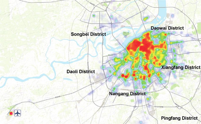
6                                                                   Journal of Advanced Transportation

                           Table 4: Selection of model lag order.
Model     LogL     AIC∗                 BIC               HQC         Adj. R-sq           Specification
39      − 87.099   3.422               3.677              3.521        0.821              ARDL (1, 3)
38      − 86.555   3.438               3.730              3.551        0.820              ARDL (1, 4)
32      − 87.018   3.455               3.747              3.568        0.817              ARDL (2, 3)
31      − 86.253   3.464               3.792              3.591        0.818              ARDL (2, 4)
37      − 86.522   3.474               3.802              3.601        0.817              ARDL (1, 5)
24      − 85.817   3.484               3.849              3.625        0.817              ARDL (3, 4)
25      − 86.999   3.491               3.819              3.618        0.813              ARDL (3, 3)
30      − 86.155   3.497               3.862              3.638        0.815              ARDL (2, 5)
23      − 85.410   3.506               3.907              3.661        0.816              ARDL (3, 5)
36      − 86.480   3.508               3.873              3.650        0.813              ARDL (1, 6)
17      − 85.710   3.517               3.918              3.672        0.814              ARDL (4, 4)
16      − 84.816   3.521               3.959              3.690        0.816              ARDL (4, 5)
15      − 83.961   3.526               4.000              3.709        0.817              ARDL (4, 6)
18      − 86.984   3.527               3.892              3.668        0.809              ARDL (4, 3)
29      − 86.083   3.530               3.932              3.686        0.811              ARDL (2, 6)
22      − 85.148   3.533               3.971              3.702        0.813              ARDL (3, 6)
40      − 91.205   3.535               3.754              3.619        0.796              ARDL (1, 2)
10      − 85.207   3.535               3.973              3.704        0.813              ARDL (5, 4)
9       − 84.646   3.551               4.025              3.734        0.812              ARDL (5, 5)
2       − 83.835   3.558               4.069              3.755        0.813              ARDL (6, 5)
3       − 84.842   3.558               4.032              3.741        0.811              ARDL (6, 4)
11      − 86.872   3.559               3.960              3.714        0.806              ARDL (5, 3)
8       − 83.949   3.562               4.073              3.759        0.813              ARDL (5, 6)
33      − 91.096   3.567               3.823              3.666        0.792              ARDL (2, 2)
1       − 83.465   3.581               4.128              3.792        0.811              ARDL (6, 6)
4       − 86.513   3.582               4.020              3.752        0.804              ARDL (6, 3)
26      − 90.783   3.592               3.884              3.705        0.790              ARDL (3, 2)
41      − 94.056   3.602               3.785              3.673        0.778              ARDL (1, 1)
34      − 93.569   3.621               3.840              3.705        0.778              ARDL (2, 1)
19      − 90.680   3.625               3.953              3.752        0.787              ARDL (4, 2)
27      − 93.562   3.657               3.912              3.756        0.773              ARDL (3, 1)
12      − 90.592   3.658               4.023              3.799        0.783              ARDL (5, 2)
42      − 97.098   3.676               3.822              3.733        0.757              ARDL (1, 0)
5       − 90.228   3.681               4.082              3.836        0.781              ARDL (6, 2)
20      − 93.506   3.691               3.983              3.804        0.769              ARDL (4, 1)
35      − 97.092   3.712               3.895              3.783        0.752              ARDL (2, 0)
13      − 93.463   3.726               4.054              3.853        0.764              ARDL (5, 1)
28      − 97.092   3.749               3.968              3.833        0.747              ARDL (3, 0)
6       − 93.242   3.754               4.119              3.895        0.761              ARDL (6, 1)
21      − 97.054   3.784               4.039              3.883        0.742              ARDL (4, 0)
14      − 97.053   3.820               4.112              3.933        0.737              ARDL (5, 0)
7       − 96.216   3.826               4.155              3.953        0.739              ARDL (6, 0)
39      − 87.099   3.422               3.677              3.521        0.821              ARDL (1, 3)
38      − 86.555   3.438               3.730              3.551        0.820              ARDL (1, 4)
32      − 87.018   3.455               3.747              3.568        0.817              ARDL (2, 3)
31      − 86.253   3.464               3.792              3.591        0.818              ARDL (2, 4)
37      − 86.522   3.474               3.802              3.601        0.817              ARDL (1, 5)
24      − 85.817   3.484               3.849              3.625        0.817              ARDL (3, 4)
25      − 86.999   3.491               3.819              3.618        0.813              ARDL (3, 3)
30      − 86.155   3.497               3.862              3.638        0.815              ARDL (2, 5)
23      − 85.410   3.506               3.907              3.661        0.816              ARDL (3, 5)
36      − 86.480   3.508               3.873              3.650        0.813              ARDL (1, 6)
17      − 85.710   3.517               3.918              3.672        0.814              ARDL (4, 4)
16      − 84.816   3.521               3.959              3.690        0.816              ARDL (4, 5)
15      − 83.961   3.526               4.000              3.709        0.817              ARDL (4, 6)
18      − 86.984   3.527               3.892              3.668        0.809              ARDL (4, 3)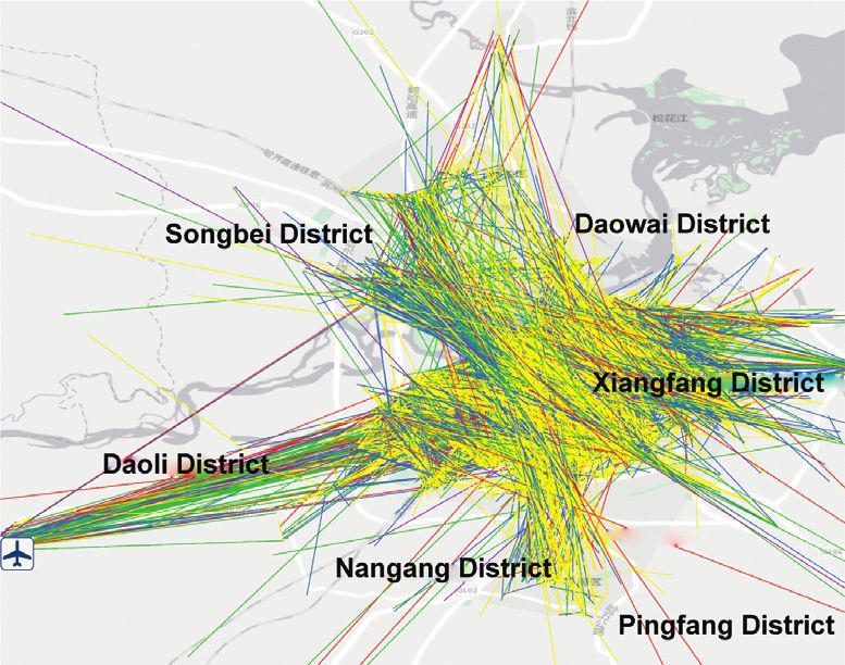
Journal of Advanced Transportation 7
Y(t) � α + βY(t − 1) + c0 X(t) + c1 X(t − 1) + c2 X(t − 2) The least square analysis was conducted on the data, and
the regression results obtained are shown in Table 5.
+ c3 X(t − 3) + η1 D1 + η2 D2 . According to Table 5, the model can be represented as
(4)
Y(t) � 0.127Y(t − 1) − 1.105X(t) − 0.689X(t − 1) − 0.534X(t − 2) − 0.492X(t − 3) + 3.112D1 + 1.925D2 + 25.886,
(5)
R2 � 0.849.
As shown in the regression results, the coefficient of the As can be seen from Figures 6 and 7, the hot spots of taxi
first lag period of variable Y is 0.127, but this coefficient is not demands are mainly distributed in residential districts of
significant, indicating that the DAOV of the previous day Rongshi, Zhaolin, Nanzhi Road, Renli, Anjing, Aijian,
will not have a significant impact on that of the day. The Xinchun, Xincheng, Anbu, Haping Road, Tongda, Hexing
coefficients of snowfall X and its lags are − 1.105, − 0.689, Road, Xinhua, Hongqi, Haxi, Jianshe, Wenfu Road and
− 0.534, and − 0.492, respectively, which are all valid at the Heilongjiang Province University, Harbin Railway Station,
significance level of 5%, indicating that snowfalls have a Harbin East Railway Station, Harbin West Railway Station,
significant negative impact on the DAOV, and the impact and Taiping International Airport. And they are all affected
lasts for about three days and decreases with time. The by the snowfall to varying degrees. Among the six days, the
regression coefficients of dummy variables D1 and D2 are most significant day is the day of snowfall (as shown in
3.112 and 1.925, respectively, and are both valid at the Figures 6(b) and 7(b)), when snowfall happened in the
significance level of 1%, indicating that the DAOV is sig- morning and might affect traffic throughout the day. As can
nificantly higher than that on weekdays due to the weekend be seen from (c), (d), (e), and (f ) in Figures 6 and 7, the taxi
effect. DAOVs on Saturday and Sunday are 3.112 and 1.925 operation was still continuously affected by the snowfall
more than on weekdays, respectively. The intercept is 25.886, within 1–3 days after the snowfall, especially within the 1-2
indicating that when there is no snowfall, the DAOV is days after, and it gradually returned to the pre-snowfall level
25.886 on average. The goodness of fit of the regression by the 4th day after the snowfall.
equation is 0.849, indicating that the data was well inter- In the hot spots of the PUPs, the most affected areas by
preted by the model. the snowfall are the residential districts of Zhaolin, Renli,
Anjing, Aijian, Xinchun, Xincheng, Anbu, Haping Road,
Tongda, Hexing Road, Xinhua, Hongqi, Wenfu Road, Haxi,
4. Discussion Jianshe, and so on. Among the hot areas at the DOPs, the
To support the results more intuitively, this study selects one residential districts of Zhaolin, Renli, Anjing, Xinchun,
of the snowy days (December 10, on which the snowfall was Tongda, Hexing Road, Wenfu Road, Haxi, and Jianshe are
3 mm, classified as heavy snow) and carried out a visual the most vulnerable areas. These areas usually have tourist
analysis on the taxi operation conditions of the day attractions (such as Anjing Residential District, where
before the snowfall (December 9), the day of the snowfall Sophia Cathedral is located) or business districts (such as
(December 10), and the four days after the snowfall residential districts of Xinchun, Hesheng Road, and Haxi),
(December 11–14). indicating that the snow mainly has a great impact on
From Figure 5, we can see that taxi demand follows a residents’ entertainment or shopping behaviors. While some
stable daily pattern with three peaks, corresponding to residential areas, such as residential districts of Rongshi and
morning, noon, and evening peak, respectively. At the same Nanzhi Road (which both had a population of more than
time, the demand getting served by hour on December 10 100,000), were not significantly affected by the snowfall,
met a significant decline due to the snowfall starting at the indicating that snowfall had less effect on residents’ daily
early morning. Note that there is a significant decline on commuting behaviors.
December 11 but not on December 12 and 13. The reason for As snow reduces the accessibility of the road, the speed of
this is that these two days are weekends, and as the model traffic flow will be significantly reduced, which results in
result shows, there is a positive weekend effect on DAOV longer trip duration than that under normal weather con-
during weekends, which offsets the negative effects of the ditions. Figure 8 shows the connection between the PUPs
snowfall. and the DOPs of all the taxi trips. Different colors represent
Due to the different nature of land use, the hot spots of different trip duration levels.
pick-up points (PUPs) and dropping-off points (DOPs) in a As can be seen from Figure 8, compared with December
city are distributed unevenly. At the same time, the heat of 9 (Figure 8(a)), the trip duration in December 10 and the
both points in the same area in different days will also be following two days (Figures 8(b)–8(d)) has increased sig-
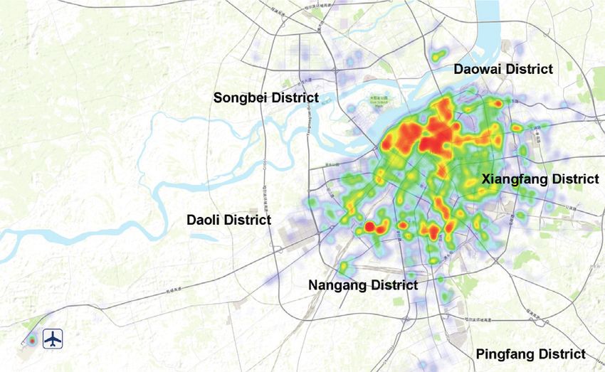
affected by weather. Figures 6 and 7, respectively, show the nificantly, especially for those airport-to-city intervals, be-
thermal diagram of the PUPs and the DOPs of taxis in cause the airport is far away from the city (33 km), and only
Harbin within the 6 days. one expressway connects the two areas. On December 13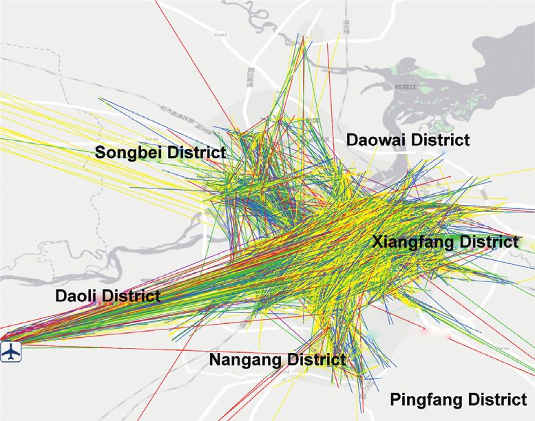
8                                                                                                                                    Journal of Advanced Transportation

                                                                   Table 5: Regression results.
Variable              Coefficient                                                   Std. error                                                 t-statistic          Prob.∗
Y(t − 1)                0.127                                                       0.114                                                       1.120             0.268
X                      − 1.105                                                      0.160                                                      − 6.895            0.000
X(t − 1)               − 0.689                                                      0.213                                                      − 3.236            0.002
X(t − 2)               − 0.534                                                      0.201                                                      − 2.651            0.011
X(t − 3)               − 0.492                                                      0.196                                                      − 2.513            0.015
D1                      3.112                                                       0.500                                                       6.223             0.000
D2                      1.925                                                       0.580                                                       3.318             0.002
C                      25.886                                                       3.400                                                       7.614             0.000

                                                  4000                                                                      1.5

                                                                                                                                  Snowfall by hour (mm)
                           Demand served hourly

                                                  3500
                                                  3000
                                                  2500                                                                      1.0
                                                  2000
                                                  1500                                                                      0.5
                                                  1000
                                                   500
                                                     0                                                                      0.0
                                                         Dec.09

                                                                      Dec.10

                                                                                 Dec.11

                                                                                                 Dec.12

                                                                                                          Dec.13

                                                                                                                   Dec.14
                                                                                          Date

                                                                  Trip demand get served
                                                                  Snowfall
                      Figure 5: Trip demand getting served in each hour during the 6 days.

           Low                                                                 High              Low                                                       High
            Airport                                                                                 Airport

                          (a)                                                                                                     (b)

           Low                                                                 High          Low                                                           High
            Airport                                                                                 Airport

                          (c)                                                                                                     (d)
                                                                      Figure 6: Continued.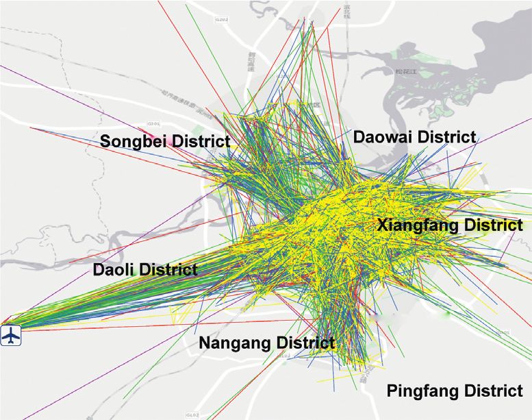
Journal of Advanced Transportation                                                                                        9

           Low                                          High     Low                                         High
            Airport                                                   Airport

                                      (e)                                                (f )

Figure 6: Spatial distribution of PUPs during the 6 days. (a) December 9, (b) December 10, (c) December 11, (d) December 12,
(e) December 13, and (f ) December 14.

                      Low                                High   Low                                 High
                            Airport                                   Airport

                                            (a)                                   (b)

                      Low                                High   Low                                 High
                            Airport                                   Airport

                                            (c)                                   (d)

                      Low                                High   Low                                 High
                            Airport                                   Airport

                                            (e)                                   (f )

Figure 7: Spatial distribution of DOPs during the 6 days. (a) December 9, (b) December 10, (c) December 11, (d) December 12,
(e) December 13, and (f ) December 14.
10                                                                                           Journal of Advanced Transportation

                      Travel time                                 Travel time
                            120 min
                           30~60 min           Airport                 30~60 min             Airport

                                         (a)                                         (b)

                      Travel time                                 Travel time
                            120 min
                           30~60 min           Airport                 30~60 min             Airport

                                         (c)                                         (d)

                      Travel time                                 Travel time
                            120 min
                           30~60 min           Airport                 30~60 min             Airport

                                         (e)                                          (f )

Figure 8: OD distributions with different trip duration levels during the 6 days. (a) December 9, (b) December 10, (c) December 11,
(d) December 12, (e) December 13, and (f ) December 14.

and 14 (Figures 8(e) and 8(f )), the duration time gradually          Interval distribution of trip duration reflects taxi trip
returned to the level before the snowfall, implying that the       duration distribution. From Figure 9, we can see that trips
snowfall had a significant effect on travel efficiency.                within 10 minutes have higher proportions during snowy
Journal of Advanced Transportation 11
0.35
0.30
0.25
Proportion
0.20
0.15
0.10
0.05
0.00
5 8 11 14 17 20 23 26 29 32
Trip duration (min)
Dec. 08 Dec. 11
Dec. 09 Dec. 12
Dec. 10 Dec. 13
Figure 9: Interval distribution of trip durations during the 6 days.
Others Others Daoli Others Dao
Da
oli ist. Dis ist. li D
st. gD t. gD ist
Di Di
fan
an .
D
g
g
st.
f
fan
ng
an
ao
Xi
Xia
wa
ng
Da
Xia
iD
owa
ist
Daowai Dist
i Dist
S o ng b ei D
S o ng b ei D
S o ng b ei D
ist .
ist .
ist .
Pi n
Pi n
Pi n
ist
gf
ng
gf
gf
ng ng
a
D
st
a
a
Di g
Di st st. g an Di Di
st. Di Na n
st. g
ng g an
Na n g a Na n
(a) (b) (c)
Others Dao Others Others Dao
ist. li D Da li D
gD ist st. oli st.
an . Di D Di is
g
g
t.
ist
f
fan
fan
ng
.
Xia
ng
ng
Da
Da
Xia
Xia
owa
owai
i Dist
Daowai Dist
Dist
S o n gb e i D
S o n gb e i D
S on g b e i
Di s
i st .
i st .
t. P
Pi n
Pi n
in
gf
gf
ng ng an
gf
ist ist
a
a
Di Di g st
st .
a ng
D st .
a ng
D Di
st. Di
g g ng
Nan Nan N an g a
(d) (e) (f )
Figure 10: OD flows in different districts of Harbin over 6 days. (a) December 9th. (b) December 10th. (c) December 11th. (d) December
12th. (e) December 13th. (f ) December 14th.
days. It can be inferred that during snowy days people would for this may be that in snowy days the traffic flow speed
be more likely to take taxis for short distance trips while decreases due to the poor road conditions, which accounts
choosing other transportation modes for middle- or long- for higher fare, and it is uneconomical to take a taxi to travel
distance trips or they even just give up such trips. The reason far-away.12 Journal of Advanced Transportation
Different regions in the city are affected by population, (4) Since snowfall will reduce the speed of traffic flow,
geography, economy, land use, and other factors. The taxi travel time will increase significantly. Especially for
travel intensity within and between regions is different and those long-distance trips, the travel efficiency is
may be affected by snowfall. In order to reflect the OD flow further reduced.
of taxis within and between the districts, a chord diagram (5) Snowfalls not only affect the trip demand in different
was proposed in this study using a circular visualization districts to different extents, but they also affect the
package, which was well adopted in the study [52]. interaction between different districts.
It can be seen from Figure 10 that Nangang District and
(6) Although some studies have considered the autor-
Xiangfang District have the highest taxi order intensity among
egression phenomenon in traffic parameters, in the
the 6 districts, and the closest travel contact happens between
study of this paper, the autoregression phenomenon
Nangang District and Xiangfang District and between Daoli
of DAOV is not significant; that is, the DAOV of that
District and Nangang District. As the residence of Hei-
day is relatively independent from that of the pre-
longjiang provincial government and more than 20 univer-
vious days.
sities, Nangang District has active economic activities, dense
population, and large traffic demand. During the snowy days, The above conclusions are of great significance, and we
the proportion of taxi demands in Nangang met an increase, give some policy suggestions from three perspectives:
and the same thing happened to the inner Nangang District. For taxi drivers, they can adjust their operation schedules
At the same time, as the location of the only airport in Harbin, according to the hot spot distribution and weekend effect, so
Daoli District has strong relationships with the other districts. as to increase the efficiency of finding passengers and in-
However, the relationships weakened in the snowy days. This crease their benefits. For example, it is advised to relocate
can be interpreted that the snowfall accounted for the flight their taxis to residential areas after the snowfall since the
delay or even cancellation, and many passengers cancelled shopping- and entertainment-related trips decrease. And
their taxi trips to the airport. This situation returned to they are advised to find potential passengers in districts like
normal within the third day after the snowfall. Nangang, Daoli, and Xiangfang.
For municipal departments, knowing the impact
mechanism of snow on taxis, they can adjust their work plan
5. Conclusions of snow clearing and deicing to minimize the impact of snow
This paper aims to study the lag effect of snowfall on taxi on urban traffic. Although the snow clearing work of Harbin
operation through taxi GPS data. First, the paper sampled municipal department is very timely and efficient, some
and cleaned the taxi trajectory data of Harbin for 61 con- minor road segments are usually given low priority in the
secutive days, so as to extract all the pick-up points and snow clearing schedule. Since these road segments also bear
drop-off points as well as the duration time of each trip from a lot of traffic volume, the snow and ice clearing work of
the daily trajectory sample data. Then, combined with the 61 these segments should not be neglected in the 3 days after
days snowfall data, an ARDL model was built to explain the snowfalls.
lag effect. Taxi daily average order volume (DAOV), which is For transportation management departments, the results
assumed to be directly proportional to taxi drivers’ benefits, of the study can provide suggestions for developing flexible
is constructed as explained variable in the model. In order to traffic scheduling schemes to facilitate the daily travel of
better understand and demonstrate the results of the model, citizens after snowfalls. Temporary bus routes should be
some visualization methods are applied to the six days before planned to serve the long-distance trips. It is also worth
and after a snowfall. From the results of the model and paying attention to ensuring the timely operation of routine
visualization, the following conclusions can be drawn: buses.
All kinds of urban public transport interrelate and in-
(1) Snow has a significant impact on the benefits of taxi teract with each other, and the traffic demand will transfer
networks and has a significant lag effect with a lag among them. To understand the impact of snowfalls on taxi
period of 3 days. From the fourth day after the operation and the overall transportation system from a
snowfall, the impact of snowfall on taxi benefits was broader perspective, data on other modes of public trans-
basically eliminated. port, such as buses and metros, may be obtained for further
(2) The snowfall has a negative impact on taxi benefits in study in the future.
various hot areas of the city, but the impact is dif-
ferent. The impact of snowfall is greater in the areas
with business concentration and less in the areas
Data Availability
with residential communities. This shows that The experiment data used to support the findings of this
snowfall has a greater impact on the travel demand study have not been made available because of participant
for shopping and entertainment. privacy and commercial confidentiality.
(3) The DAOV on weekends is significantly higher than
that on weekdays; that is, the demand for taxis on
Conflicts of Interest
weekends is more vigorous, and taxi drivers are
expected to have higher benefits on weekends. The authors declare no conflicts of interest.Journal of Advanced Transportation 13
Acknowledgments Infrastructure Engineering, vol. 36, no. 12, pp. 1530–1548,
2021.
The study has been funded by National Key R&D Program of [16] M. Hofmann and M. O’Mahony, “The impact of adverse
China (no. 2019YFB2102702). weather conditions on urban bus performance measures,” in
Proceedings of the 2005 IEEE Intelligent Transportation Sys-
tems, pp. 84–89, Vienna, Austria, September 2005.
References [17] D. Jaroszweski and T. McNamara, “The influence of rainfall
on road accidents in urban areas: a weather radar approach,”
[1] P. Arana, S. Cabezudo, and M. Peñalba, “Influence of weather
Travel Behaviour and Society, vol. 1, no. 1, pp. 15–21, 2014.
conditions on transit ridership: a statistical study using data
[18] E. Chung, O. Ohtani, H. Warita, M. Kuwahara, and H. Morita,
from Smartcards,” Transportation Research Part A: Policy and
“Effect of rain on travel demand and traffic accidents,” in
Practice, vol. 59, pp. 1–12, 2014.
Proceedings of the 2005 IEEE Intelligent Transportation Sys-
[2] A. Singhal, C. Kamga, and A. Yazici, “Impact of weather on
tems, pp. 1080–1083, Vienna, Austria, September 2005.
urban transit ridership,” Transportation Research Part A:
[19] C. Pennelly, G. W. Reuter, and S. Tjandra, “Effects of weather
Policy and Practice, vol. 69, pp. 379–391, 2014.
on traffic Collisions in edmonton, Canada,” Atmosphere-
[3] H. Kojo, P. Leviäkangas, R. Molarius, and A. Tuominen,
“Extreme Weather Impacts on Transport Systems,” Espoo, Ocean, vol. 56, no. 5, pp. 362–371, 2018.
[20] K. El-Basyouny, S. Barua, and M. T. Islam, “Investigation of
no. 168, pp. 1–136, 2011.
[4] M. J. Koetse and P. Rietveld, “The impact of climate change time and weather effects on crash types using full Bayesian
and weather on transport: an overview of empirical findings,” multivariate Poisson lognormal models,” Accident Analysis &
Transportation Research Part D: Transport and Environment, Prevention, vol. 73, pp. 91–99, 2014.
vol. 14, no. 3, pp. 205–221, 2009. [21] D. Chen, Y. Zhang, L. Gao, N. Geng, and X. Li, “The impact of
[5] A. K. Andersson and L. Chapman, “The impact of climate rainfall on the temporal and spatial distribution of taxi
change on winter road maintenance and traffic accidents in passengers,” PloS one, vol. 12, Article ID e0183574, 2017.
West Midlands, UK,” Accident Analysis & Prevention, vol. 43, [22] P. Thaker and S. Gokhale, “The impact of traffic-flow patterns
no. 1, pp. 284–289, 2011. on air quality in urban street canyons,” Environmental Pol-
[6] B. Aamaas, J. Borken-Kleefeld, and G. P. Peters, “The climate lution, vol. 208, pp. 161–169, 2016.
impact of travel behavior: a German case study with illus- [23] H. Budnitz, L. Chapman, and E. Tranos, “Better by bus?
trative mitigation options,” Environmental Science & Policy, Insights into public transport travel behaviour during
vol. 33, pp. 273–282, 2013. StormDorisin Reading, UK,” Weather, vol. 73, no. 2,
[7] M. Hyland, C. Frei, A. Frei, and H. S. Mahmassani, “Riders on pp. 54–60, 2018.
the storm: exploring weather and seasonality effects on [24] H. Xiao, H. Sun, and B. Ran, “Special factor adjustment model
commute mode choice in Chicago,” Travel Behaviour and using fuzzy-neural network in traffic prediction,” Trans-
Society, vol. 13, pp. 44–60, 2018. portation Research Record: Journal of the Transportation Re-
[8] L. Böcker, M. Dijst, and J. Prillwitz, “Impact of everyday search Board, vol. 1879, no. 1, pp. 17–23, 2004.
weather on individual daily travel behaviours in perspective: a [25] T. Nosal and L. F. Miranda-Moreno, “The effect of weather on
literature review,” Transport Reviews, vol. 33, pp. 71–91, 2013. the use of North American bicycle facilities: a multi-city
[9] S. Najafabadi, A. Hamidi, M. Allahviranloo, and N. Devineni, analysis using automatic counts,” Transportation Research
“Does demand for subway ridership in Manhattan depend on Part A: Policy and Practice, vol. 66, pp. 213–225, 2014.
the rainfall events?” Transport Policy, vol. 74, pp. 201–213, [26] S. Zhang, H. Wang, X. Liu, and W. Quan, “Dynamic impact of
2019. meteorological factors on freeway free-flow volume and speed
[10] L. Ma, H. Xiong, Z. Wang, and K. Xie, “Impact of weather in Yanbian,” Procedia - Social and Behavioral Sciences, vol. 96,
conditions on middle school students’ commute mode pp. 2667–2675, 2013.
choices: empirical findings from Beijing, China,” Trans- [27] W. Qiao, A. Haghani, and M. Hamedi, “Short-term travel
portation Research Part D: Transport and Environment, time prediction considering the effects of weather,” Trans-
vol. 68, pp. 39–51, 2019. portation Research Record: Journal of the Transportation Re-
[11] Y. Wang, Y. Bie, and Q. An, “Impacts of winter weather on search Board, vol. 2308, no. 1, pp. 61–72, 2012.
bus travel time in cold regions: case study of Harbin, China,” [28] G. Yannis and M. G. Karlaftis, “Weather effects on daily traffic
Journal of Transportation Engineering, Part A: Systems, accidents and fatalities: a time series count data approach,” in
vol. 144, no. 11, Article ID 05018001, 2018. Proceedings of the 89th Annual Meeting of the Transportation
[12] S. A. Kashfi, J. M. Bunker, and T. Yigitcanlar, “Modelling and Research Board 2004, p. 14, MD, USA, July 2004.
analysing effects of complex seasonality and weather on an [29] D. Eisenberg, “The mixed effects of precipitation on traffic
area’s daily transit ridership rate,” Journal of Transport Ge- crashes,” Accident Analysis & Prevention, vol. 36, no. 4,
ography, vol. 54, pp. 310–324, 2016. pp. 637–647, 2004.
[13] J. Corcoran and S. Tao, “Mapping spatial patterns of bus usage [30] T. Brijs, D. Karlis, and G. Wets, “Studying the effect of weather
under varying local temperature conditions,” Journal of Maps, conditions on daily crash counts using a discrete time-series
vol. 13, no. 1, pp. 74–81, 2017. model,” Accident Analysis & Prevention, vol. 40, no. 3,
[14] J. Zhao, C. Guo, R. Zhang, D. Guo, and M. Palmer, “Impacts pp. 1180–1190, 2008.
of weather on cycling and walking on twin trails in Seattle,” [31] R. Billot, N.-E. El Faouzi, and F. De Vuyst, “Multilevel as-
Transportation Research Part D: Transport and Environment, sessment of the impact of rain on drivers’ behavior,”
vol. 77, pp. 573–588, 2019. Transportation Research Record: Journal of the Transportation
[15] Y. Bie, J. Ji, X. Wang, and X. Qu, “Optimization of electric bus Research Board, vol. 2107, no. 1, pp. 134–142, 2009.
scheduling considering stochastic volatilities in trip travel [32] T. Nosal and L. F. Miranda-Moreno, “Cycling and Weather: A
time and energy consumption,” Computer-Aided Civil and Multi-City and Multi-Facility Study in North America,” in14 Journal of Advanced Transportation
Proceedings of the Transportation Research Board annual economic growth interactions in India: the ARDL bounds
Meeting, Washington DC, USA, January 2012. testing approach,” Procedia - Social and Behavioral Sciences,
[33] N. S. Arunraj and D. Ahrens, “Estimation of non-catastrophic vol. 104, pp. 914–921, 2013.
weather impacts for retail industry,” International Journal of [49] P. Lingras, S. C. Sharma, P. Osborne, and I. Kalyar, “Traffic
Retail Distribution Management, vol. 44, no. 7, pp. 0959–0552, volume time-series analysis according to the type of road use,”
2016. Computer-Aided Civil and Infrastructure Engineering, vol. 15,
[34] Z.-Y. Zhan, Y.-M. Yu, T.-T. Chen, L.-J. Xu, S.-L. An, and no. 5, pp. 365–373, 2000.
C.-Q. Ou, “Effects of hourly precipitation and temperature on [50] Y. Zhang and Y. Zhang, “A comparative study of three
ambulance response time,” Environmental Research, vol. 181, multivariate short-term freeway traffic flow forecasting
Article ID 108946, 2020. methods with missing data,” Journal of Intelligent Trans-
[35] H. M. P. S Government, “Harbin statistical yearbook,” 2016, portation Systems, vol. 20, no. 3, pp. 205–218, 2016.
http://www.harbin.gov.cn/col/col39/index.html. [51] W. Wang, H. Zhang, T. Li et al., “An interpretable model for
[36] N. Takahashi, S. Miyamoto, and M. Asano, “Using taxi GPS to short term traffic flow prediction,” Mathematics and Com-
gather high-quality traffic data for winter road management puters in Simulation, vol. 171, pp. 264–278, 2020.
evaluation in Sapporo, Japan,” in Proceedings of Sixth Inter- [52] H. Wang, H. Huang, X. Ni, and W. Zeng, “Revealing spatial-
national Symposium on Snow Removal and Ice Control temporal characteristics and patterns of urban travel: a large-
Technology, pp. 455–469, Transportation Research Board, scale analysis and visualization study with taxi GPS data,”
Washinton DC, USA, June 2004. ISPRS International Journal of Geo-Information, vol. 8, no. 6,
[37] S. Zhang, J. Tang, H. Wang, Y. Wang, and S. An, “Revealing p. 257, 2019.
intra-urban travel patterns and service ranges from taxi
trajectories,” Journal of Transport Geography, vol. 61,
pp. 72–86, 2017.
[38] L. Wu, S. Hu, L. Yin et al., “Optimizing cruising routes for taxi
drivers using a spatio-temporal trajectory model,” ISPRS
International Journal of Geo-Information, vol. 6, no. 11, p. 373,
2017.
[39] Y. Wang, K. Qin, Y. Chen, and P. Zhao, “Detecting anomalous
trajectories and behavior patterns using hierarchical clus-
tering from taxi GPS data,” ISPRS International Journal of
Geo-Information, vol. 7, no. 1, p. 25, 2018.
[40] L. Tang, F. Sun, Z. Kan, C. Ren, and L. Cheng, “Uncovering
distribution patterns of high performance taxis from big trace
data,” ISPRS International Journal of Geo-Information, vol. 6,
no. 5, p. 134, 2017.
[41] G. Yang, C. Song, H. Shu, J. Zhang, T. Pei, and C. Zhou,
“Assessing patient bypass behavior using taxi trip origin-
destination (OD) data,” ISPRS International Journal of Geo-
Information, vol. 5, no. 9, p. 157, 2016.
[42] P. S. Castro, D. Zhang, and S. Li, “Urban traffic modelling and
prediction using large scale taxi GPS traces,” in Proceedings of
International Conference on Pervasive Computing, pp. 57–72,
CA, USA, May 2012.
[43] C. Yang and E. J. Gonzales, “Modeling taxi demand and
supply in New York city using large-scale taxi GPS data,” in
Springer Geography Seeing Cities through Big Data, pp. 405–425,
Springer, Berlin, Germnay, 2017.
[44] P. K. Narayan, “Fiji’s tourism demand: the ARDL approach to
cointegration,” Tourism Economics, vol. 10, no. 2, pp. 193–206,
2004.
[45] S. A. Hassan and M. Nosheen, “The impact of air trans-
portation on carbon dioxide, methane, and nitrous oxide
emissions in Pakistan: evidence from ARDL modelling ap-
proach,” International Journal of Innovation and Economic
Development, vol. 3, no. 6, pp. 7–32, 2018.
[46] P. Stamolampros and N. Korfiatis, “Airline service quality and
economic factors: an ARDL approach on US airlines,” Journal
of Air Transport Management, vol. 77, pp. 24–31, 2019.
[47] M. K. Khan, J.-Z. Teng, and M. I. Khan, “Effect of energy
consumption and economic growth on carbon dioxide
emissions in Pakistan with dynamic ARDL simulations ap-
proach,” Environmental Science and Pollution Research,
vol. 26, no. 23, Article ID 23490, 2019.
[48] R. P. Pradhan, N. R. Norman, Y. Badir, and B. Samadhan,
“Transport infrastructure, foreign direct investment andYou can also read