Households income and the cushioning effect of fiscal policy measures during the Great Lockdown

Households´ income and the cushioning
effect of fiscal policy measures during
the Great Lockdown

 JRC Working Papers on
 Taxation and Structural
 Reforms No 06/2020

 Vanda Almeida, Salvador Barrios, Michael
 Christl, Silvia De Poli, Alberto Tumino and
 Wouter van der Wielen

 August 2020

This p ublication is a Technical re port by the Joint Research Ce ntre (JRC), the European Commission’s science and knowledge service. It
aims to p rovide evidence-based scientific support to the European p olicymaking process. The scientific output e xpressed does not imp ly a
p olicy p osition of the European Commission. Neither the European Commission nor any p erson acting on behalf of the Commission is
re sp onsible for the use that might be made of this publication. For information on the me thodology and quality underlying the data used
in this p ublication for which the source is neither Eurostat nor other Commission service s, users should contact the re ferenced sou rce. The
de signations employed and the p resentation of material on the maps do not imp ly the exp ression of any opinion whatsoever o n the p art
of the European Union concerning the le gal status of any country, territory, city or are a or of its authoritie s, or concernin g the delimitation
of its frontie rs or boundaries.

EU Science Hub
http s://ec.europa.eu/jrc

JRC121598

Se ville : European Commission, 2020

© Europ ean Union, 2020

The re use p olicy of the European Commission is imp le mented by the Commission Decision 2011/833/EU of 12 December 2011 on the
re use of Commission documents (OJ L 330, 14.12.2011, p . 39). Exce pt otherwise noted, the re use of this document is authorised under
the Cre ative Commons Attribution 4.0 International (CC BY 4.0) lice nce (http s://cre ativecommons.org/licenses/by/4.0/). This me ans that
re use is allowed p rovided appropriate cre dit is give n and any changes are indicated. For any use or re production of photos or other
mate rial that is not owned by the EU, permission must be sought directly from the copyright holders.

All conte nt © European Union, 2020.

How to cite this re p ort: Alme ida V., Barrios S., Christl M., De Poli S., Tumino A. and van der Wie le n W. (2020), Households´ income and the
cushioning effect of fiscal p olicy me asures during the Gre at Lockdown, JRC Working Papers on Taxation and Structural Reforms No
06/2020, European Commissio n, Joint Research Ce ntre, Seville . JRC121598

Households´ income and the cushioning effect of
fiscal policy measures during the Great Lockdown1

Vanda Almeida, Salvador Barrios, Michael Christl,
Silvia De Poli, Alberto Tumino and Wouter van der Wielen
Joint Research Centre, European Commission.

Abstract

We analyse the impact of the COVID-19 crisis on EU households´ income and assess the cushioning
effect of discretionary policy measures taken by the EU Member States. Our assessment is bas ed on
the European Commission Spring 2020 forecasts and counterfactual scenarios under a no policy-
change assumption. Our analysis suggests that over the course of 2020, on average, households’
disposable income in the EU would fall by -5.9% due to the COVID-19 crisis without discretionary
policy measures, and by -3.6% with policy intervention, pointing to a significant cushioning effec t of
these measures in protecting households against income losses. Furthermore, our results confirm that
the impact of the COVID-19 crisis is likely to be highly regressive, with the poorest households´
being the most severely hit. However, discretionary policy measures are expected to contain the
regressive effects of the recession, resulting in a quite homogeneous impact along the income
distribution. Poverty, as measured by the at risk of poverty (AROP) rate, would increase significantly,
even in presence of policy measures (+1.7pp), although this result depend on whether we anc hor the
poverty line to its pre-crisis level. When not doing so, the impact of the COVID crisis on poverty
becomes very close to the one observed in the aftermath of the financial crisis (i.e. +0.1pp) once
policy measures are considered. Given the sheer size of the COVID shock, we might consider that the
anchored poverty line may provide a more reliable assessment of the impact of the Great lockdown on
poverty, however. Policy interventions are therefore seen as instrumental in cushioning against the
impact of the crisis on inequality and poverty. Finally, our results suggest that the social impact of the
Great Lockdown is likely to be much larger than the one experienced during the 2008/2009 financ ial
crisis, at least for what concerns the immediate impact of the crisis.

1
 Corresponding author: Michael.CHRISTL@ec.europa.eu.
 We are thankful to comments on earlier preliminary results received from Olivier Bontout, Peter Benc zur ,
 Daniel Daco, Lucie Davoine, Giulio Paso and Sergio Torrejón Pérez. The views expressed in this paper should
 not be attributed to the European Commission.

 1

1. Introduction

Preliminary indicators on job destruction and unemployment benefits claims across European
Union (EU) countries suggest that the impact of the COVID-19 pandemic on households will
in all likelihood be exceptionally high (OECD, 2020).2 Early findings suggest that the risk of
job loss is highest in southern Europe and France (Doerr and Gambacorta, 2020). At the
country level, young, low-educated, low-income workers appear to face the highest income
and employment risk (see Pouliakas and Branka (2020) for the EU; Galasso (2020) for Italy;
Adams-Prassl et al. (2020b) for Germany; Bradley et al. (2020) for the UK; Beland et al.
(2020), Cajner et al. (2020), Cho and Winters (2020), Mongey et al. (2020) and Shibata
(2020) for the US; and Aum et al. (2020) for South Korea).3 For example, Joyce and Xu
(2020) find that low earners in the UK are seven times as likely as high earners to have
worked in a sector shut down following the lockdown. The consequences of the COVID-19
crisis on households´ income in particular, although unknown with precision yet, raise serious
concerns.

Policies aimed at protecting those most directly hit by the crisis, either through discretionary
measures (e.g., income subsidies or tax rebates), or through automatic stabilisation (e.g.
unemployment benefits or lower taxes paid as a result of job loss and/or decrease in market
incomes), could partly reduce the toll on household income and consumption.4 Recent
evidence from Denmark (Bennedsen et al., 2020), for instance, shows that without
government support, in the form of labour subsidies, firms are expected to have proceeded
with layoffs instead. In addition, Chetty et al. (2020) find that stimulus payments to low-
income households in the US increased consumer spending sharply.5

The existing evidence suggests that Covid-19 crisis will lead to an increase in both poverty
and wage inequality in all European countries. Palomino et al. (2020), for instance, estimate
the Gini coefficient to increase 2.2% in all Europe. Moreover, historic data suggest that past
events of this kind, even though much smaller in scale, have led to significant, persistent
increases in the net Gini coefficient (by 1.25% five years after the pandemic) and raised the
income shares of higher income deciles (Furceri et al., 2020). Therefore, a micro-based

2 OECD (2020), Evaluating the initial impact of COVID-19 containment measures on economic activity,
Organisation for Economic Cooperation and Development, Paris.
3 Two groups moreover seem relatively more affected by the Great Lockdown vis-à-vis the Gl obal Financial

Crisis (Shibata, 2020): (i) Women were about one third more likely to work in a sector that is now shut down
(Joyce and Xu, 2020); and (ii) Non-whites (i.e. Hispanics and blacks), see e.g. Bel a nd et a l . (2 0 20), Cho a nd
Winters (2020), Cowan (2020) and Fairlie et al. (2020), and immigrants, see e.g. Borjas & Cassidy (2020), all for
the US. Platt and Warwick (2020) document a similar vulnerability of Pakistanis and Bangladeshis in the UK.
4 Nevertheless, many individuals would remain vulnerable if ensured 50% of thei r gr oss pr ivatel y ea r ned

income (Midões, 2020). In the EU, at least 99 million individuals live in households that cannot cover for two
months of the most basic expenses only from their savings in bank accounts.
5 The authors find none to modest short-run employment effects. One possible explanation is that firms have

almost entirely stopped posting new vacancies; see e.g. Costa Dias et al. (2020) for the UK and Campello et a l .
(2020) for the US. Similarly, many of those losing their jobs are currently also not (yet) looking for new ones
(Coibion et al., 2020).

 2

distributional analysis of the Great Lockdown and the cushioning policies – like the one done
by Figari and Fiorio (2020) for Italy, Bronka et al. (2020) and Brewer and Tasseva (2020) for
the UK and O’Donogue et al. (2020) and Breine et al. (2020) for Ireland – covering the whole
EU is warranted to inform policy decisions.

This paper provides an assessment of the potential impact of policy measures adopted in the
wake of the COVID-19 crisis on household income, poverty and inequality in the EU in
2020. We take into account the macroeconomic scenarios included in the European
Commission Spring 2020 forecasts. These forecasts embed the impact of discretionary policy
measures taken or announced by governments, including those financed thanks to EU
support, following the COVID-19 outbreak, and of automatic stabilisers reflecting the
existing features of each member state’s tax and transfer system. To obtain estimates for GDP
growth in a world with no discrete policy measures, we construct a counterfactual no policy-
change scenario based on estimates for the budgetary impact of these measures (taken from
the Stability and convergence programmes) together with estimates on spending and revenue
fiscal multipliers taken from the literature. For each of these scenarios, we compute and
compare households’ income, inequality and poverty indexes, which allows us to estimate the
overall impact of the crisis and the cushioning effect of discretionary measures.

We use EUROMOD, the microsimulation model for the EU, to compute the impact of
aggregate GDP and employment changes on households’ incomes. One of the many
advantages of EUROMOD is that it enables a consistent EU-wide application and
comparison. The lack of up-to-date household survey data on incomes for each of the
scenarios, however, poses a methodological challenge. We overcome this by applying a
reweighting approach (somewhat similar to O’Donogue et al., 2020; and Breine et al., 2020),
which reweights the underlying EUROMOD survey micro data from the European Statistics
on Income and Living Conditions (EU-SILC) to mimic the aggregate employment and
unemployment figures, as well as other macroeconomic targets in each scenario. The
advantage of our approach is that we can precisely introduce changes in the population
structure of the survey data, introducing observed labour market trends into our micro data.
This allows us to analyse the impact of not only employment and unemployment changes, but
also the micro impact of the wage compensation schemes covered by the macro information
(e.g. total wage compensation). It is important to note that EUROMOD is a static model, i.e.
it only measures the impact of policy and income changes without making assumption about
behavioural effects. Given that our analysis focuses on the immediate consequences of the
COVID crisis, this seems a rather reasonable assumption.

Our main findings are twofold. First, our simulations show that EU member states’ policy
interventions have been instrumental in cushioning against the early impact of the crisis on
inequality and poverty. Second, to put our results into perspective, we also provide a direct
comparison of the simulated impact of the Great Lockdown to the social impact experienced
during in the aftermath of the Great Recession starting in 2008. Our results suggest that the
social impact of the Great Lockdown is expected to be much larger than experienced during
the Great Recession, at least for what concerns the immediate impact of the crisis.
 3

The rest of the paper is organised as follows. Section 2 describes the methodology used in the
analysis. Section 3 presents the main findings. Section 4 concludes and discusses some policy
implications.

2. Methodology

2.1. Macroeconomic scenarios

We build two alternative macroeconomic scenarios expressed in terms of differences to a
scenario in which COVID-19 did not happen. First, we compare the Commission 2020
Spring forecasts and the Commission 2019 Autumn Forecast to derive information on the
estimated impacts of the COVID-19 crisis, including the shutdown of major parts of the
economy, as well as policy measures taken by Member States to counteract the strong impact
of the pandemic. In detail, we compare the changes in employment, unemployment and total
wage compensation, expected for 2020 in the Spring 2020 forecast with those expected for
the same year in the Autumn 2019 forecast.

Second, we consider a counterfactual “COVID without discretionary fiscal policy measures”,
or no policy-change, scenario, which allows us to gauge the effect of policy measures taken
by EU countries to cushion the impacts of the COVID-19 crisis. This counterfactual no
policy-change scenario consists of estimating GDP growth and changes in employment if no
discretionary policy measures had been taken to mitigate the socio-economic consequences
of the COVID-19 pandemic, and only automatic stabilisers would be at play. Consistent with
the first scenario, the changes in employment from the counterfactual scenario are compared
to those reported in the Commission 2019 Autumn forecasts to derive the effects of the
COVID-19 pandemics in absence of discretionary policy measures.

Both these scenarios are analysed by reweighting the baseline 2019 EUROMOD simulations,
applying the predicted changes in target variables. Our results are then reported in terms of
difference between the scenarios with (or without) discretionary policy measures and the
hypothetical scenario without COVID-19.6

To construct the counterfactual policy scenario, we start by estimating the GDP growth that
would be observed in the absence of policy measures. We do this by removing the expected
economic effect of COVID-19 related discretionary measures from the Commission Spring
Forecasts for GDP growth in 2020, in three main steps. The first step involves obtaining
estimates of the budgetary impact of COVID-19 related discretionary policy measures. For
national spending and revenue measures, we use the 2020 Stability and Convergence

6Intuitively, the scenario is equivalent to the following: i) reweight EUROMOD 2019 Baseline using the 2 0 19
Commission Autumn Forecast; ii) reweight EUROMOD 2019 Baseline using the 2 0 2 0 Commission Spring
forecast; iii) reweight EUROMOD 2019 Baseline using the predicted changes i n the a l ter native s cenario;
compare ii) with i) and iii) with i).

 4

Programmes (SCP) submitted by the EU Member States.7 In the same vein, we include EU-
funded public spending through the European Structural and Investment Funds (ESIF) and
the Coronavirus Response Investment Initiative (CRII), since they make up a significant
share of spending measures in some Member States. 8 The exact amounts for the EU-funded
spending by Member States were obtained from the European Commission (EC)’s
Directorate General (DG) BUDG. Loans and guarantees ensuring businesses’ liquidity are
disregarded as either they have no direct budgetary impact or their economic impact is highly
uncertain. A summary of the budgetary impact of all the discretionary policy measures
removed in the counterfactual scenario is presented in Figure 1.

Figure 1: COVID-19 related discretionary measures with a budgetary impact in 2020

Note: includes spending and revenue measures and EU-level spending, excludes guarantees

It is important to note that the counterfactual scenario solely corrects for discretionary
measures taken in response to the pandemic, which include only newly introduced policies or
significant change to existing policies. For example, for countries that already had wage
compensation schemes in place before the crisis (e.g. the Cassa Integrazione in Italy) and did

7 The only exception is the Netherlands, since the Dutch Stability Programme did not report any es timates of
COVID-19 related measures. Instead, data were taken from the Nether l ands Bur eau for Ec onomic Policy
Analysis (CPB) her June projections.
8
 As this mainly concerns a re-orientation of existing EU funds – in contrast to the future rec overy pac kage –
their distribution across Member States follows the existing agreements, wi th a foc us on newer Member
States.

 5

not change the scheme significantly, the automatic changes in spending with these schemes is
not included in Figure 1. Similarly, some countries reported large volume effects in the
existing unemployment scheme (e.g. Belgium), which are not included. Therefore, the no-
policy counterfactual does not allow for conclusions on the impact of automatic stabilisers.
Nevertheless, we follow this approach for two important reasons. First, using one, heavily
standardized, source (cf. the SCPs) allows for the best possible consistent comparison across
countries of our final results. Second, since the counterfactual builds on the Spring 2020
Forecast, it is suitable to rely on the same set of information used to construct said forecast.

The second step involves obtaining estimates of fiscal multipliers, using results from well-
established academic contributions, in order to obtain a set of representative small, average
and large multipliers. 9 This results in an average multiplier close to, but below, one for public
spending – in line with the calibration of the QUEST model. Similarly, the resulting average
multiplier for the overall budget balance (0.8) is closely in line with, although slightly above,
the average multiplier used in the recommendations under the EU’s excessive deficit
procedure in the recent past. 10 Using the annual values for the multipliers obtained from the
literature, we estimate quarterly values, by making assumptions on the intensity of the impact
of policy measures in each stage of the observed/expected progression of lockdown
measures. We consider three possible scenarios for the quarterly evolution of the multipliers,
a low, a medium and a high scenario. The multipliers considered in each quarter in each of
the three scenarios are presented in Figure 2.

We start from an average multiplier in the first quarter of 2020 as no or little lockdown
measures were in place. In the second quarter, the multiplier is assumed to drop considerably
in the low scenario, slightly drop in the medium scenario and stay the same in the high
scenario, reflecting different possibilities for the severity of the impact of lockdown
measures. The impact of discretionary fiscal measures is then expected to strengthen in the
third quarter, as lockdown measures are lifted and a possible overshooting of consumption
may be observed, with a small increase in the multiplier in the low scenario, a big increase in
the medium scenario, and a very big increase in the high scenario. Finally, the situation is
assumed to reverse to values closer to the average in the fourth quarter, staying exactly on
average in the low scenario, slightly above average in the medium scenario and well above
average in the high scenario.

The third step involves multiplying the estimated budgetary impact of the discretionary
budget measures (as a percentage of GDP) by the estimated fiscal multipliers, to obtain the

9 For example, Gechert (2015) provides a comprehensive meta-analysis of spending and revenue mul tipliers
estimated using both macroeconometric models as well as structural models. Coenen et al. (20 12 ) r ec oncile
the fiscal multipliers from seven prominent structural policy models, including those by the European Centr al
Bank (NAWM), the European Commission (QUEST), the IMF (GIMF) and the OECD (OECD Fiscal). Kilponen et al.
(2019), in their turn, look across the dynamic macro models used by the member institutions of the European
System of Central Banks. Finally, van der Wielen (2020) documents recent, empirical estimates, with a
particular focus on the EU.
10 As documented by Gόrnicka et al. (2018), the average multiplier between 2012 and 2015 amounted to 2/3.

 6

GDP impact of these measures, for each of the three multiplier scenarios, low, medium and
high. The result of this multiplication is subtracted from DG ECFIN’s Spring Forecasts for
GDP growth, resulting in three no policy-change scenarios for GDP growth, as summarised
in Figure 3. As can be seen, discretionary policy measures are expected to play a considerable
role in mitigating the recessionary impact of the pandemic, with GDP growth for the EU
average being between 1.4 and 3.5 percentage points lower in the no policy-change scenario.

Figure 2: Budget balance multipliers used for 2020 no policy-change scenarios

Figure 3: 2020 GDP growth - Commission 2020 Spring Forecast vs. No Policy-change
Scenarios

 7

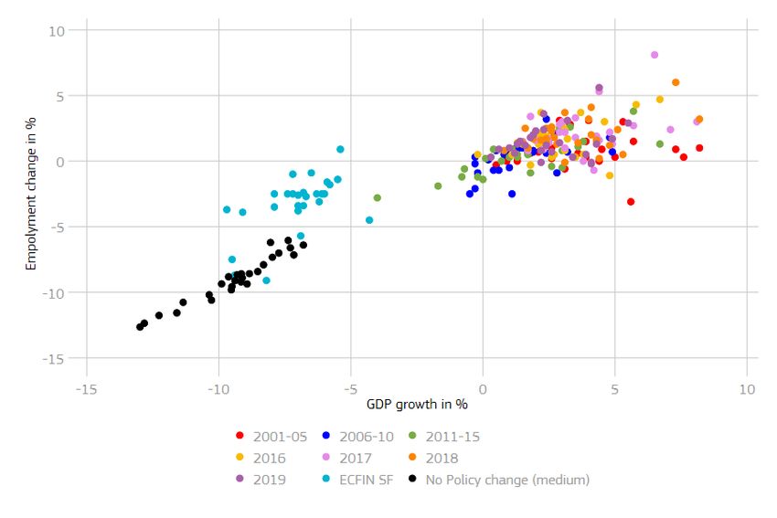
Finally, to implement the no policy-change scenario in the microanalysis, the estimated GDP
growth values are translated into an expected impact on employment (expressed in
comparison to employment changes reported in the Commission 2019 Autumn forecast). The
Trade-SCAN model – see e.g. Román et al. (2019) – is used twice to do this. First, the whole
economy GDP estimates are brought to the sectoral level using the latest sectorial distribution
estimated in Trade-SCAN, e.g. accounting for the relatively large burden of the overall shock
on sectors such as “Accommodation and food services”. Second, using the GDP -employment
relationship by sector inherent in the Trade-SCAN model, the sectoral GDP changes are
translated into sectoral employment changes. Lastly, the sectoral employment changes are
aggregated to obtain aggregate employment changes for each Member State. The results for
the aggregate employment changes in each of the scenarios, together with the employment
changes considered in the Commission Spring forecasts can be seen in Table A2 in the
Annex, together with a depiction of the relationship between GDP growth and employment
changes underlying the estimates in the different scenarios in Figure A1.

2.2. EUROMOD

Our analysis makes use of EUROMOD, the EU microsimulation model, version I2.0+.
Making use of representative survey data from the European Statistics on Income and Living
Conditions (EU-SILC), the model is a static tax-benefit calculator, designed to provide results
which are representative at the country-level and validated against aggregate national
statistics. The model simulates the personal income taxes, social benefits and social security
contributions in all EU countries and can be used to study the effect of actual and perspective
policy reforms on household incomes, inequality, poverty and the government’s fiscal
balance11.

The scope of EUROMOD simulations includes direct taxes and non-contributory benefits in
place in each country as of 30 June 2019. Some contributory benefits, such as unemployment
benefits, are also simulated in most countries, making assumptions on working history for
eligibility purposes where needed. In countries where simulations of unemployment benefits
are not satisfactory, the value recorded in the underlying EU-SILC data is used instead.
Consistent with the 2020 Spring forecasts, this paper takes into account the impact of short
term working (STW) schemes on wages.

We apply our reweighting methodology to EUROMOD simulations based on data from 2017
EU-SILC, containing incomes of 2016, and 2019 policy system (see Annex 4 for further
details on this approach).12 Non simulated tax-benefit instruments are uprated to their 2019

11For a detailed description of EUROMOD and of the scope of its simulation see Figari and Sutherland (2013).
12In a number of countries, the national version of SILC has been used either directly or to c omplement the
information contained in the EU-SILC UDB distributed by EUROSTAT.

 8

values making use of specific uprating factors (see EUROMOD Country Reports 2019 for
more information on the data used and uprating factors). 13

2.3. Reweighting – Introducing the macro shock at the micro level

To perform the analysis using EUROMOD, we reproduce the 2020 macroeconomics
scenarios previously described in the EU-SILC data, which underlies the datasets used by
EUROMOD. To do this, we rely on a reweighting approach, using it to translate the changes
in several aggregate variables present in the macroeconomic scenarios into changes at the
microeconomic level.

To estimate the size of the aggregate shock in the scenario with discretionary policy changes,
we consider the differences between the Commission Autumn forecasts (before the COVID-
19 outbreak) and the Spring forecast (after the outbreak) for the year 2020. The
counterfactual scenario focuses on differences between Commission Autumn forecasts for the
year 2020 and “modified” Spring forecast for the same year, i.e. excluding the employment
consequences of the discretionary policy changes. We then introduce these shocks into the
micro data, following the reweighting approach proposed by Pacifico (2014), which we
summarise below

Formally, let us consider a survey of N individuals and K individual-level variables, such as
income, gender, working status and age: , = ( ,1 , ,2 , … , , ). The survey weight is
defined as a vector = ( 1 , 2 , … , ) of all individual weights. The estimated 1 × K vector
of survey totals is given by:
 
 = ∑ ∗ 
 =1

Since we are interested in introducing a shock into our data, we are particularly interested in
changes to specific group totals (while other population characteristics might stay the same)
to get a realistic dataset for 2020 that includes our shock. It is possible to compute a new
vector of survey weights = ( 1 , 2 ,… , ) that is as close as possible to the original
weights and that respects the following calibrating conditions,
 
 = ∑ ∗ 
 =1

where is the 1 × K vector of projected total values including the shock. Let us assume
that the distance between the original and the new weights is following a distance function
 ( , ), then the new weights can be obtained by minimising a Lagrangian function with
respect to the new weights:

13
 https://www.euromod.ac.uk/using-euromod/country-reports.

 9

 

 = ∑ ( , ) + ∑ ∗ ( − ∑ ∗ , )
 =1 =1 =1

where = ( 1 , 2 , … , ) are the Lagrange multipliers. The solution of the minimization
problem depends on the properties of the chosen distance function. We use the distance
function proposed by Deville and Särndal (1992) which keeps the calibrated weights within a
known range set.14

In sum, the proposed approach follows the three steps below:

 1) The macroeconomic forecast scenarios are used to change the micro data used in
 EUROMOD in accordance with the employment shock in each country. The number
 of employed is reduced accordingly, while the number of unemployment recipients is
 increased. Additionally, to account for wage compensation schemes and potential
 wage losses, in the scenario with discretionary policy changes we also adjust for the
 expected change in total wage compensation of employees and self-employed in each
 country. In the alternative scenario, i.e. in absence of discretionary policy changes, the
 total wage bill will change only as a consequence of the unemployment increase.

 2) Reweighting at the household level is used to introduce a new micro structure in the
 unemployed population that reflects the micro structure of the shock scenario. The
 target number of unemployed, as derived in the first step, is recreated in the EU-SILC
 data. Detailed information can be found in Table 1.

  We reweight total employment and total wage receivers, given the changes
 that are projected by the differences in the Autumn 2019 and Spring 2020
 forecasts.
  We reweight total unemployment and total unemployment benefit receivers,
 given the reduction in employment observed.
  In the scenario with discretionary policy changes, we adjust the wage
 compensation of employees in our data given the expected shock on wages.
 This measure accounts for wage compensation schemes. We also adjust the
 total wage compensation of self-employed.
  We ensure that the population structure stays the same, by controlling for
 several age groups (0-15 years, 16 to 40, 41-65 years, as well as 65+) as well
 as for gender shares.

 3) Individual unemployment benefits as well as personal income taxes, social insurance
 contributions and other benefits from the reweighted simulation of EUROMOD are
 aggregated at the country level to analyse the impact of the changes on the labour
 market (unemployment, wage loss) on households’ income. This leads to a forecast of
 the macro statistics that correspond to the given shock.

14
 For more information, see Pacifico (2014).

 10

Our approach allows us to generate a new dataset that is not only similar in expected
employment shocks due to COVID-19, but also in terms of the impact on wages, including
wage compensation schemes. Our EUROMOD baseline policy system is 2019. We do the
reweighting based on the expected percentage change in the macro-economic variables of
interest.

Table 1: Shock translation into EUROMOD
 Information EUROMOD shock/constant
 employment increase (farmer, self- les=1,2,3 shock
 employed, employees)
 employment income receivers yem>0 & shock
 yem>ils_b1_bun
 Unemployment les=5 shock
 unemployment benefit receivers ils_b1_bun>0 shock
 Labour market
 structure Pensioners les=4 constant
 Students les=6 constant
 Inactive les=7 constant
 sick or disabled les=8 constant
 other labour market status les=9 constant
 Wage Yem Shock
 wage self employed Yse Shock
 Gender Dgn constant
 demographic population group (0-15) Dag constant
 characteristics population group (16-40) Dag constant
 population group (41-65) Dag constant
 population group (>65) Dag constant

 11

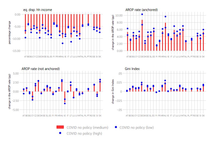
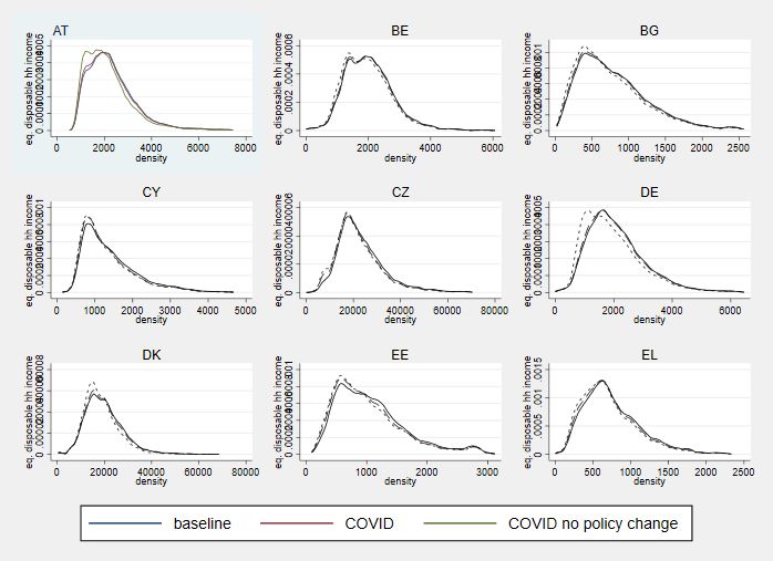
3. Main findings

In this section, we present the main results of our analysis on the impact of the COVID-19
crisis, obtained by comparing the two COVID scenarios, with and without discretionary
policy measures. Section 3.1 contains EU level analysis, excluding Poland and Romania due
to data limitation.15 Section 3.2 contains country specific results. Here we consider only the
medium scenario for the “COVID without policy changes” scenario, leaving the analysis of
the low and high scenarios for future work.

3.1. Impact of COVID-19 on household income, inequality and poverty at the EU-level

Figure 4 provides results on the impact of COVID-19 on households´ equivalised disposable
income by income decile in the EU, for the two COVD scenarios considered. On average,
household income would fall by -5.9% due to the impact of COVID-19 without policy
measures, while policy intervention reduces this impact to -3.6%. In absence of policy
responses, the COVID-19 pandemic would have a clear regressive effect on households´
income, with the poorest households´ being the most hardly hit. The first three lowest income
deciles would experience a fall in net disposable income oscillating between -9.0% and 8.6%.
The fall in income for the highest income deciles (deciles 8-10) would represent
approximately only half of the falls experienced by the bottom income deciles: between -
5.2% and -3.9%. The COVID pandemic would therefore affect households disproportionally,
affecting poorest household much more severely, although all households would potentially
experiment a fall in their disposable income. Looking at the policy change scenario, we can
see that the measures taken by government lead to a reduction of the regressive effect,
resulting in a homogeneous impact of about -4% all along the income distribution. This
highlights that policy measures taken by the governments to counteract the regressive effect
of the COVID crises are likely to be quite effective.

Figure 4 shows that observations in the richest decile would be worse off in the scenario
taking into account discretionary policy changes than in the one not taking them into account.
The result is driven by the fact in the latter scenario only changes in
employment/unemployment are taken into account in the reweighting, while in the scenario
with discretionary policy changes also the changes in the total wage compensation are
considered. Intuitively, in the scenario with discretionary policy changes households suffer
less from unemployment, but more from the reduction in wage compensation. This explains
why richest households experience, in our setting, a larger reduction in disposable income
that they would in absence of discretionary policy changes.

15
 The analysis excludes Poland and Romania. Romania is excluded because of the significant underreporting of
unemployment benefits in the EUROMOD input datasets. Poland is excluded because the dr op in the tota l
wage compensation arising from the comparison between Commission Autumn 2019 and Spring 2020
Forecasts significantly outweighs the predicted change in employment. This appears to be at odds with theor y
and the observed trends in other countries.

 12

Figure 4: Impact of COVID-19 on household disposable income in the EU

Note: The impact of COVID-19 concerns 2020 (source: EUROMOD simulation) and is estimated using household
net disposable income by income decile. Households ranking is based on the income distribution of each
scenario (baseline, Counterfactual and Spring forecast). Results are weighted (population) average of co u ntry
results.

Figure 5 provides a synthetic view on the impact of the COVID crisis on income inequality
by reporting the Gini index obtained according to the two simulated scenarios, and comparing
these results with the impact of the 2008/2009 financial crisis. 16 This figure shows a number
of important results. First, in absence of policy responses, the COVID-19 pandemic would
trigger a substantial increase in inequality, as measured by the Gini index. This increase is
expected to be 3.6%. Policy measures, however, are able to counteract the inequality
increasing effect of the COVID pandemic to a large extent, as inequality in the scenario
including policy measures would fall by 0.7%.17 As a matter of fact, the 2008/2009, similarly
led to a small decrease in income inequality on average for the EU (-0.3%, sources: Eurostat
and authors´ calculations).

16
 Note that the starting level of the Gini index is taken from Eurostat and concerns the year 2018 (year t in the
graph) which is the latest available year covering all EU countries. The simulated percentage c hanges i n the
Gini index are obtained from EUROMOD and applied to this value. The Gini indices for the income reported in
years 2008 and 2009 are taken from the same Eurostat database.
17
 Results on Gini are likely to be influenced by the high impact of policy changes on high income households.
As explained above, this result might be driven by the fact that in the scenario with policy changes , we
consider not only changes in unemployment but also the reduction in wage compensation.

 13

Figure 5: Impact of COVID-19 on income inequality in the EU

Note: The impact of COVID-19 concerns the year 2020 (source: EUROMOD simulation). The starting level of the
Gini index is the weighted (population) average for 2018 (Source: Eurostat, EU-SILC database). The imp a ct o f
the 2008/2009 crisis compares households´ net disposable income between these two years (Source: Euro stat,
EU-SILC database). Year t corresponds to 2019 for the COVID crisis and to 2008 for the 2008/2009 crisis.

Figure 6 provides evidence on the potential impact of COVID-19 on poverty, measured by
the at risk of poverty (AROP) rate (using the 60% of median income as threshold), and
compares the simulated effect of the COVID crisis with the 2008/2009 crisis. These results
are obtained by anchoring the poverty lines to their 2019 values. According to the results, the
AROP rate would increase significantly due to the COVID pandemic, moving from 16.8%
(2018 data, source: EUROSTAT) on average in the EU, up to 21.6% (no policy change).
When we account for policy measures, this increase is less pronounced, from 16.8% to
18.5%. By comparison, the 2008/2009 crisis implied much lower increases in the AROP rate,
from 16.2 to 16.3%, i.e. +0.1 percentage point (+1% in terms of percentage variation).

Figure 7 provides evidence on the potential impact of COVID-19 on poverty, measured by
the at risk of poverty (AROP) rate (using the 60% of median income as threshold), when we
do not anchor the poverty line to the pre-crisis level. Again, the AROP rate would increase
significantly due to the COVID pandemic, but to a smaller extent. Policy measures can
almost offset this increase in the AROP rate. When analysing this results we have to keep in
mind that the poverty line drops substantially in this analysis due to the income shock of the
COVID crisis.

Given the sheer size of the COVID shock we might consider that the anchored poverty line
may provide a more reliable assessment of the impact of the Great lockdown on poverty.

 14

Figure 6: Impact of COVID-19 on poverty in the EU

Note: The impact of COVID-19 concerns 2020(source: EUROMOD simulation). The starting level o f th e A ROP
indicator is the weighted (population) average for 2018 (Source: Eurostat, EU-SILC database). The impact of the
2008/2009 crisis compares AROP indicator between these two years (Source: Eurostat, EU-SILC database). The
year t corresponds to 2019 for the COVID crisis and to 2008 for the 2008/2009 crisis.

Figure 7: Impact of COVID-19 on poverty (non-anchored) in the EU

Note: The impact of COVID-19 concerns 2020(source: EUROMOD simulation). The starting level o f th e A ROP
indicator is the weighted (population) average for 2018 (Source: Eurostat, EU-SILC database). The impact of the
2008/2009 crisis compares AROP indicator between these two years (Source: Eurostat, EU-SILC database). The
year t corresponds to 2019 for the COVID crisis and to 2008 for the 2008/2009 crisis.

3.2. Country-specific results

Additionally to the aggregate results at the EU-level, this subsection takes a closer look at the
distributional impacts of the COVID-19 crisis, considering each of the EU member states
separately. Our reweighting methodology introduces some uncertainty in the model, since we
 15

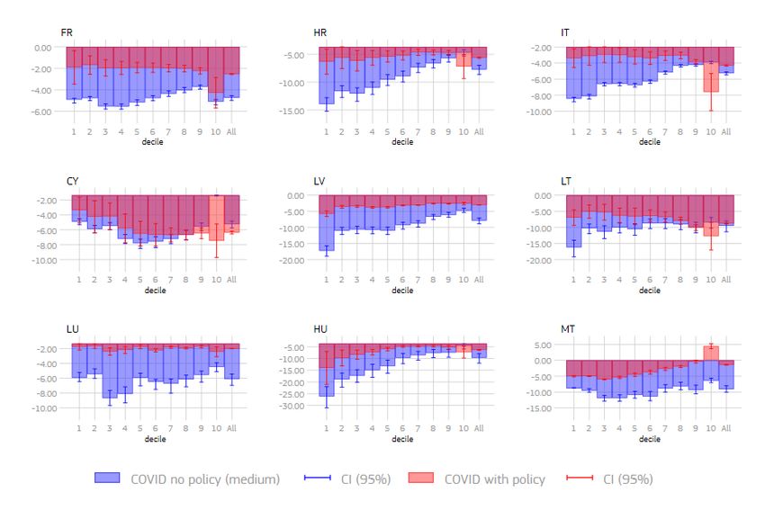
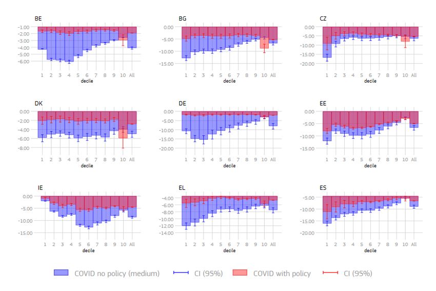
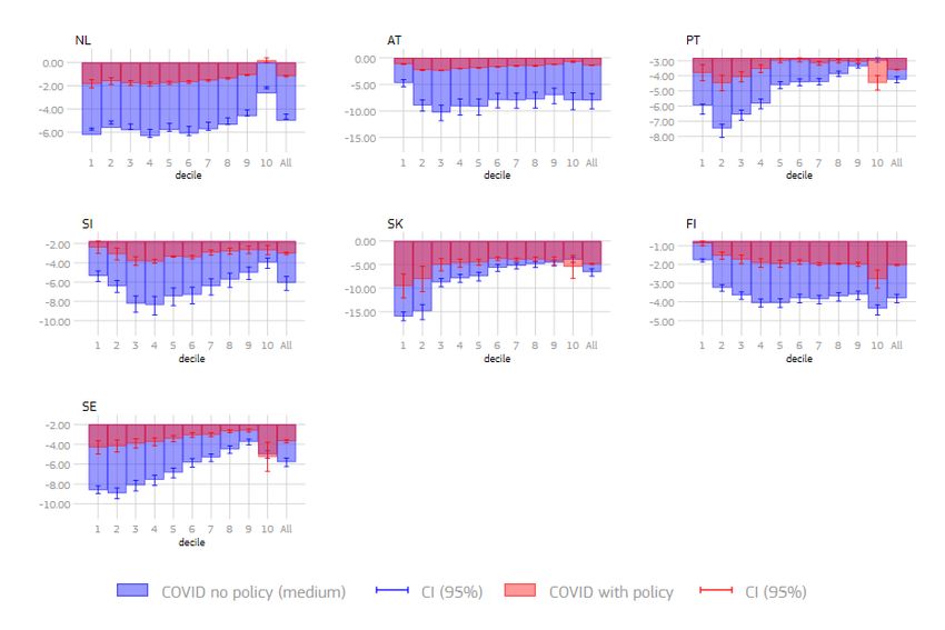
could end up with different solutions, when we reweight our population. Therefore, we report
the confidence intervals of our report by using a bootstrapping method (see section 3.3 for an
in-depth discussion).

Figure 8 shows the impact of the COVID-19 crisis on household equivalised disposable
income. We consider first the medium policy scenarios (i.e. taking average values of the
fiscal multipliers as indicated in Section 2.1). The income loss is expected to be especially
high in countries such as Austria, Germany, Denmark, Spain, Hungary, Ireland, Lithuania
and Malta. Still, policy measures can offset this income loss substantially. In countries such
as Austria, Germany, Denmark, Malta and the Netherlands, policy measures taken can reduce
the income losses substantially. Despite the policy measures, we expect the biggest impact of
the COVID pandemic on equivalised disposable household income in countries such as
Bulgaria, Spain, Estonia, Croatia, Hungary and Lithuania. For Cyprus, there is also no
difference in the replacement rate between wage compensation and unemployment benefits,
which potentially explain the results.

Figure 8: Impact of the COVID-19 crisis on equivalised disposable household income in EU
countries

Additionally, we can also see that there is substantial uncertainty in our methodology
regarding some countries (see Figure A5 in the Annex), therefore an interpretation of the
results for those countries have to be taken with extreme care. Considering the low and high
scenarios (corresponding to low and high fiscal multipliers) instead would not significantly
change the interpretation of our results concerning the no-policy change scenarios, although
in some cases the impact of the crisis would be rather pronounced under the high scenarios
 16

compared to the medium one (as in the case of Austria, Germany, Denmark, Hungary or
Lithuania, for instance).

Figure 9 shows the impact of the COVID crisis on poverty, measured by the AROP rate,
where the poverty line is anchored to the value of the 2019 EUROMOD baseline simulations.
Not surprisingly, the AROP rate jumps substantially in the counterfactual scenario, where no
policy measures are taken. This is due to a substantial household income decrease due to the
strong increase in unemployment that differs across countries. Substantial increases of over
5pp in the AROP would take place in many member states due in absence of policy
interventions. Especially high poverty rates would be observed in the hypothetical scenario
with no policy intervention (blue bars) in Germany, Bulgaria, Spain, Hungary and Latvia.
Strong increases can be also seen in Malta, Austria and Slovakia. When we consider the
policy measures taken by the governments, we can see that the impact of COVID on the
AROP rate can be alleviated in many countries and in some even almost offset, particularly in
Germany, Denmark, Finland, France and Luxemburg.18

Figure 9: Impact of the COVID-19 crisis on poverty (AROP rate) in EU countries

18
 If we consider the non-anchored poverty rate in Figure A4 in the Annex, we can see that the impa ct on the
poverty rate is not as strong as in the case of an anchored poverty rate. The results are driven by a substantial
drop of the poverty line in both, the COVID scenario with and without policy measures compared to baseline.
As Figure 7 already showed, both shock scenarios lead to a severe reduction in equivalised disposable
household income, shifting the income distribution and therefore the poverty line to the left. Keepi ng this i n
mind it is not surprising that in the case of the shock scenarios, the non-anchored poverty r ea cts l ess to the
COVID shocks than the non-anchored one.

 17

Figure 10 shows the impact of the COVID crisis on inequality, measured by the Gini index.
In most countries, policy measures are able to offset the inequality-increasing pattern of the
COVID pandemic, but there are some exceptions. For example in Austria, Denmark, Estonia,
Spain and Malta policy measures can only partially attenuate the increase in the Gini index. It
is also worth noting that in some countries, the confidence intervals are quit large, such as in
Eastern European countries, such as Bulgaria, Czechia and Hungary.

The above results are driven by the impact of the COVID shock on household income. While
in the scenario of COVID without policy measures all people losing their job are sent to
unemployment, in the case of the COVID scenario with policy measures, the government
tries to counteract the loss in household income by policies such as wage compensation
schemes. To get a clearer picture on the impacts on the income distribution, we additionally
take a closer look at the impacts on household income by income decile in each country, see
figures A5 in the Annex. We can see that in most of the countries, policy measures can offset
the regressive impact of the COVID pandemic, but still we can see that there is substantial
uncertainty in our results when it comes to the impact on the top and the bottom part of the
income distribution.

Figure 10: Impact of the COVID-19 crisis on inequality (Gini index) in EU countries

3.3. Robustness of the country specific results

We must acknowledge that our approach faces some limitations, due to the need to make
strong assumptions regarding the way the macroeconomic shock related to the COVID-19 is

 18

translated at the micro-level and in the determination of the baseline scenario. We have
conducted a number of robustness check in order to address these limitations.

First, we use the policy system of 2019, with underlying EU-SILC data from 2017 (income
year 2016) which are uprated to 2019 prices. Second, the concept of expenditures and
revenues of EUROMOD might be different to standard national accounting concepts that are
used on macro level. To overcome both problems, we stick to reporting and using percentage
changes when introducing the shock in the data.

Our method generates a new population (given the expected labour market and demographic
changes) due to reweighting. Therefore, we are not able to follow the same person in both
populations. We have to change the income deciles accordingly when comparing scenarios.
This approach is in line with comparing changes over years.
When we introduce the unemployment shock, we assume that all new unemployed have
similar characteristics as the current unemployment pool. Hence, we cannot take into account
the fact that the newly unemployed might differ from the pool of currently unemployed. It
should also be noted that reweighting may perform worse compared to a transition approach
in times of rapid economic changes, e.g. if individuals entering in unemployment have
characteristics completely different from the characteristics of the unemployed observed in
the base year.
Furthermore we do not have information on which employees are especially hit by a wage
loss (that also stems from short-time working schemes). By using a reweighting approach, the
survey weights of employees with higher wages are shifted to employees with lower wages.
This approach does not take into account any distributional pattern that wage loss could
potentially have. Other studies show, that essential workers are often based in the lower
income deciles, while home-office possibilities are typically more likely for high-income
earners, see for instance Galasso (2020) for an analysis specific to the COVID pandemic on
labour markets. Hence, there is evidence that people in the middle-upper part of the
distribution are more likely to move to short-time work. Additionally, since we do not
explicitly simulate compensation schemes but we rather reweight to take them into account,
the potentially heterogeneous effect of these schemes across the income distribution (like e.g.
upper limits in the wage compensation schemes, which lead to higher wage drops in the
upper income distribution) are also not considered in our approach.

To ensure the robustness of our results, we introduce a bootstrapping procedure that allows
the algorithm to be more flexible in the weight choice. In the baseline, the algorithm specifies
the upper and lower bound of the ratio between the new and the original weight when the
Deville and Sarndal's distance function is used. To ensure that the choice of the boundaries
does not affect our solution, we do bootstrapping on randomly chosen bounds in the

 19

algorithm.19 Therefore, we get a sequence of results that allow us to build an average effect
with a standard error.

The bootstrapping procedure allows us to test the statistical significance of our results. The
confidence intervals are represented in all the country specific figures, and additionally, Table
A4 in the Annex summarizes the standard errors in the EU-27 for specific indicators. We can
see that these standard errors are especially high in countries such as Cyprus, Lithuania,
Czechia and Hungary. Additionally, we can see that when looking at the distributional
country-specific analysis, the uncertainty of the results is especially high in those countries
and especially in the higher deciles. This is driven by the fact that the share of employees,
who are those hit by the crises (either by losing their job or going into wage compensation) is
the highest in the upper deciles in most countries. This limitation must be taken into account
when considering our results on the distributional effects of our different scenarios.

We must also keep in mind that our approach randomly reduces wages, although the COVID-
shock might hit specific groups of worker (high-skilled vs low-skilled, male vs. female,
young vs. old), and sectors differently. Our simulations capture sector composition of the
change in employment/unemployment when converting the GDP shock into employment
shocks without considering the differential wage impact across sectors, see Section 2.

Using information available in the EU-SILC data on sector of activity we can partially
account for these effects. In such case the differential impact of the crisis by worker category
would reflect only the sectoral differences in skill/gender/age composition of the workforce.
This is consistent with Fana et al. (2020) who argue that the sectorial impact of the crisis
affects substantially the distributional impact. These authors show that those sectors that were
closed or only partly active have on average lower wages than those that were likely to be
essential or where teleworking was possible. Consequently, the sectorial structure of the
shock can potentially have an important impact on the income distribution that we do not
account for.

Those patterns seem to be quite similar across countries, as highlighted in Table A3 in the
Annex. Therefore, as an additional robustness check, we consider the impact on the wage loss
(wage compensation) only in those sectors that are mostly affected by the COVID-19
pandemic. Following Fana et al. (2020) those are: Construction, Wholesale and retail, Hotels
and restaurants and Transport and communication.

Figure 11 compares the results of our simulations on the impact of COVID-19 on
households´ income in our main scenario (including policy measures) with a scenario where
the sector dimension is considered as described above. In some cases the simulated change in
households´ disposable income is larger or smaller than in our main results. These differences
are arguably very small, however. For instance, the largest difference in results can be
observed for Sweden (+0.33pp) indicating a larger (in absolute terms) decrease in

19
 In the baseline, the value default for the upper bound is 3 and for the lower bound 0.2.

 20

households´ disposable income, which represents only a very small portion of the simulated
fall (-3.68%) in our main results. Results at decile level reveal the same type of results and
leave the distributional pattern of COVID across countries broadly unchanged compared to
our main results too20.

Figure 11: Accounting for sector specific shocks: differences in households´ disposable
income in benchmark results vs. results incorporating sector-specific impact of COVID-19

Figure 12 highlights the impact of the sector allocation on the AROP rate as well as on the
Gini compared to our benchmark results incorporating the impact of policy change. Not
surprisingly, the impact on both measures is quite similar in all countries, since both, the
AROP and the Gini are measures of income inequality. While in most countries, the sector
specific shock would lead to a higher AROP rate and Gini coefficient, in some the opposite
holds true. While the increase in both measures is especially high for Bulgaria, Spain, Ireland,
Latvia, for Czechia, Germany and Hungary we see a substantial decrease in both the Gini and
the AROP rate, when we use a sector specific shock.

Additionally to those robustness checks, Figure A3 in the Annex highlights the impact of the
assumptions underlying the macroeconomic scenario on which the counterfactual scenario in
section 2.1 is constructed. We conclude that the country-specific impact can differ
substantially depending on the choice of the multipliers when creating the counterfactual
scenarios. Using multipliers to the higher end of the spectrum (as often found for recessions
in narratively identified empirical models), for instance, would result in considerably more
negative growth rates in the counterfactual scenario. Nonetheless, the physical lockdown of

20
 Only for the 1 st and 10th decile results can vary more for some countries.

 21

economies is likely to have temporarily limited marginal propensities to consume and, thus,
the size of the multiplier for the fiscal impulses enacted in this period.

Figure 12: Accounting for sector specific shocks: differences in inequality and poverty in
benchmark results vs. results incorporating the sector-specific impact of COVID-19

4. Conclusion

The consequences of the COVID-19 crisis on households´ income, although still unknown
with precision, raise serious concerns. In this paper, we provided an assessment of the
potential impact of the policy measures adopted in the wake of the COVID-19 crisis on
household income, poverty and inequality in the EU in 2020. In particular, we used the
EUROMOD microsimulation model for the EU to compute the impact of aggregate GDP and
employment changes on households’ incomes.

We built our results around two macroeconomic scenarios. The first scenario corresponds to
the Commission 2020 Spring Forecast, including the estimated impacts of the COVID-19
crisis, such as the shutdown of major parts of the economy as well as policy measures taken
by Member States to counteract the strong impact of the pandemic. The second scenario is a
no policy-change scenario, excluding discretionary fiscal policy measures. This hypothetical
scenario is built to gauge the effect of the policy measures taken by EU countries. Both
scenarios are evaluated in terms of differences with the economy in absence of COVID-19.

 22

Next, we reweighted the underlying EUROMOD survey micro data from the European
Statistics on Income and Living Conditions (EU-SILC) to mimic the aggregate employment
figures in each scenario. In particular, we make use of the information on employment and
unemployment changes in the forecasts, as well as changes in the total wage compensation
for employees and the self-employed to simulate the impact of COVID on (un)employment,
as well as on wage compensations.

Our analysis suggests that over the course of 2020, on average, households’ disposable
income in the EU would fall by -5.9% due to the COVID-19 crisis without discretionary
policy measures, and by -3.6% with policy intervention, pointing to a significant cushioning
effect of these measures protecting households against income losses. Furthermore, our
results confirm that the impact of the COVID-19 crisis is likely to be highly regressive, with
the poorest households´ being the most severely hit. However, discretionary policy measures
are expected to contain the regressive effects of the recession. Policy interventions are
therefore instrumental to cushion against the impact of the crisis on inequality and poverty.

In addition to the aggregate results at EU-level, we presented results for each of the EU
member states. Despite some exceptions, member states’ policy measures prove their worth
in limiting poverty and inequality at the country level. Poverty, as measured by the at risk of
poverty rate (AROP) rate, would increase significantly in absence of policy measures.
However, when accounting for the policy measures taken by the governments we observe
that the impact of COVID on the AROP rate can be alleviated in many countries and in some
almost offset, especially in Germany, Denmark, Finland, France and Luxemburg. In most
countries, policy measures are able to offset the inequality-increasing pattern of the COVID
pandemic, with some exceptions. For example, in Estonia and Spain policy measures can
only partially alleviate the increase in the Gini index.

Finally, our results suggest that the social impact of the Great Lockdown is likely to be much
larger than experienced during the Great Recession, at least for what concerns the immediate
impact of the crisis. According to our results, we expect the AROP rate to increase
significantly due to the COVID pandemic: from 16.8% to 18.6% with or 21.4% without
policy measures. By comparison, the 2008/2009 crisis implied much lower increases in the
AROP rate, from 16.2% to 16.3%. Finally, it should be noted that these results are obtained
when anchoring the poverty rate to its pre-crisis level, which seems the most appropriate way
of measuring it given size of the COVID shock. When considering a non-anchored poverty
line, our results suggest that the increase in poverty would be much more contained and
comparable to the one observed in the immediate aftermath of the 2008/2009 crisis, however.

 23

References

Adams-Prassl, A., Boneva, T., Golin, M., and Rauh, C. (2020). Inequality in the Impact of the Coronavirus
 Shock: Evidence from Real Time Surveys . IZA Working Paper 13183, IZA - Institute for Labor Eco n omics ,
 Bonn.
Aum, S., Lee, S. Y. and Shin, Y. (2020). COVID-19 doesn’t need lockdowns to destroy jobs: The effect of local
 outbreaks in Korea, NBER Working Paper 27264, National Bureau of Economic Research, Cambridge (US).
Beirne, K., Doorley, K., Regan, M., Roantree, B. and Tuda, D. (2020). The Potential Costs and Dis t rib ut io nal
 Effect of Covid-19 Related Unemployment in Ireland. EUROMOD Working Paper 05/20, Institute for So cial
 and Economic Research, University of Essex, Essex, UK.
Beland, L.-P., Brodeur, A. and Wright, T. (2020). COVID-19, Stay-At-Home Orders and Employment:
 Evidence from CPS Data, IZA Working Paper 13282, IZA - Institute for Labor Economics, Bonn.
Bennedsen, M., Larsen, B., Schmutte, I. and Scur, D. (2020). Preserving job matches during the COVID-19
 pandemic: Firm-level evidence on the role of government aid, Covid Economics, 27, 1-30.
Borjas, G. J. and Cassidy, H. (2020). The adverse effect of the COVID-19 labor market shock on immigrant
 employment, NBER Working Paper 27243, National Bureau of Economic Research, Cambridge (US).
Bradley, J., Ruggieri, A., and Spencer, A. H. (2020). Twin peaks: Covid -19 and the labor market, Covid
 Economics, 29, 164-192.
Brewer, M. and Tasseva, I. (2020). Did the UK policy response to Covid -19 protect household incomes?.
 EUROMOD Working Paper 12/20, Institute for Social and Economic Research, University of Es s ex, Es s ex,
 UK.
Bronka, P., Collado, D., and Richiardi, M. (2020). The Covid-19 crisis response helps the poor: The
 distributional and budgetary consequences of the UK lockdown, Covid Economics, 26, 79-106.
Cajner, T., Crane, L. D., Decker, R. A., Grigsby, J., Hamins -Puertolas, A., Hurst, E., Kurz, C. and Yildirmaz, A.
 (2020). The U.S. Labor Market During the Beginning of the Pandemic Recession, BFI Working Pap er 2020-
 58, Becker Friedman Institute, University of Chicago, Chicago (US).
Campello, M., Kankanhalli, G. and Muthukrishnan, P. (2020). Corporate hiring under COVID-19: Labour
 market concentration, downskilling, and income inequality, NBER Working Paper 27208, National Bureau o f
 Economic Research, Cambridge (US).
Chetty, R., Friedman, J. N., Hendren, N., Stepner, M. and the Opportunity Insights Team (2020). How Did
 COVID-19 and Stabilization Policies Affect Spending and Employment? A New Real-Time Economic
 Tracker Based on Private Sector Data. Opportunity Insights Working Paper.
Cho, S. J. and Winters, J. V. (2020). The Distributional Impacts of Early Employment Losses from COVID-19,
 IZA Working Paper 13266, IZA - Institute for Labor Economics, Bonn.
Coenen, G., Erceg, C. J., Freedman, C., Furceri, D., Kumhof, M., Lalonde, R., Laxton, D., Lindé, J.,
 Mourougane, A., Muir, D., Mursula, S., de Resende, C., Roberts, J., Roeger, W., Snudden, S., Trab an d t, M .
 and in ‘t Veld, J. (2012). Effects of Fiscal Stimulus in Structural Models, American Economic Journal:
 Macroeconomics, 4(1): 22-68.
Coibion, O., Gorodnichenko, Y. and Weber, M. (2020). Labor markets during the COVID-19 crisis: A
 preliminary view, NBER Working Paper 27017, National Bureau of Economic Research, Cambridge (US).
Costa Dias, M., Norris Keiller, A., Postel-Vinay, F., and Xu, X. (2020). Job vacancies during the Covid-19
 pandemic, IFS Briefing Note 289, Institute for Fiscal Studies, London.
Cowan, B. W. (2020). Short-run effects of COVID-19 on U.S. worker transitions, NBER Working Paper 27315,
 National Bureau of Economic Research, Cambridge (US).
Deville, J.-C., and C.-E. Särndal. 1992. Calibration estimators in survey sampling.Journal of the American
 Statistical Association87: 376–382

 24