House Price Determinants and Market Segmentation in Boulder, Colorado: A Hedonic Price Approach
←
→
Page content transcription
If your browser does not render page correctly, please read the page content below

House Price Determinants and Market
                                                   Segmentation in Boulder, Colorado:
arXiv:2108.02442v1 [econ.GN] 5 Aug 2021

                                                       A Hedonic Price Approach
                                                                         Mahdieh Yazdani†
                                                                           August 6, 2021

                                                                               Abstract
                                                   In this research we perform hedonic regression model to examine the
                                               residential property price determinants in the city of Boulder in the state
                                               of Colorado, USA. The urban housing markets are too compounded to
                                               be considered as homogeneous markets. The heterogeneity of an urban
                                               property market requires creation of market segmentation. To test whether
                                               residential properties in the real estate market in the city of Boulder are
                                               analyzed and predicted in the disaggregate level or at an aggregate level we
                                               stratify the housing market based on both property types and location and
                                               estimate separate hedonic price models for each submarket. The results
                                               indicate that the implicit values of the property characteristics are not
                                               identical across property types and locations in the city of Boulder and
                                               market segmentation exists.

                                               keywords: Urban housing market, Real estate market appraisal, House
                                               price indexes.

                                            † Department of Economics,    Colorado University at Boulder.         Email contact:
                                          mahdieh.yazdani@colorado.edu
Contents

1 Introduction                                1

2 Related Literature                          2

3 Hedonic Price Model                         3

4 Data                                        5

5 Aggregate and Disaggregate Market Levels   10

6 Results                                    16

7 Conclusion                                 23

References                                   25

A Appendix                                   A1

1    Introduction
    House is one of the essentials for human beings to rest and gather with
family. In most families dwelling is one of the most important components
of a household’s wealth (see e.g., Arvanitidis (2014)). Consequently, to make
informed decisions the need for efficient and accurate real estate market price
prediction models is apparent.

    The price of any residential property is affected by many property factors
such as its structural, neighbourhood, and spatial attributes. To predict future
dwelling valuations the development of accurate housing valuation and prop-
erty price prediction models is essential (see e.g., Fan et al. (2018)). Hedonic
price models have been a common approach to analyze and predict real estate
assets. A hedonic method is trying to explain the value of a composite good
by decomposing its attributes and estimating their marginal contribution or
implicit valuations (see e.g., Rosen (1974)). The hedonic price approach has
been extensively employed in many different fields of research, and these studies
are often used by policy makers and economists for the analysis of differentiated
goods like housing whose individual features do not have explicit market prices.

    Rosen (1974) used the hedonic regression models in the field of real estate
and urban economics. Thereafter, residential hedonic analysis has become widely
used as an assessment tool to model real estate markets (see e.g., Blomquist
and Worley (1981), Milon et al. (1984), Haase et al. (2013), Jiang et al. (2014),
Del Giudice et al. (2017), Waltl (2018), and Król (2020)). The residential hedonic
price approach has been utilized in the property market literature to investigate
the relationship between house prices and housing attributes. The primary inter-
ests for such an application are improving the precision of house price indexes
and providing methods for property value estimates (see e.g., Sheppard (1999)).

   In this paper we follow the hedonic price approach to develop property ap-
praisal models in the city of Boulder, Colorado. In the city of Boulder, a popular
mountain city, with nearly 16, 701 inhabitants, buying a house is considered as
one of the most profitable investments and most people in Boulder know the
benefit of owning a house.

    Development of a dwelling price prediction method can significantly improve
the efficiency of the housing market. This study brings about some general
implications for actual and potential homeowners, property developers, investors,
tax assessors, appraisers, brokers, mortgage lenders, banks, and policy mak-
ers (see e.g., Frew and Jud (2003)). The contributions of this paper are as follows:

• Collecting real estate datasets from different resources consisting of Multiple
  Listing Service (MLS) database, Public School Ratings, Colorado Crime Rates
  and Statistics Information, CrimeReports, WalkScore, and US Census Bureau.

                                         1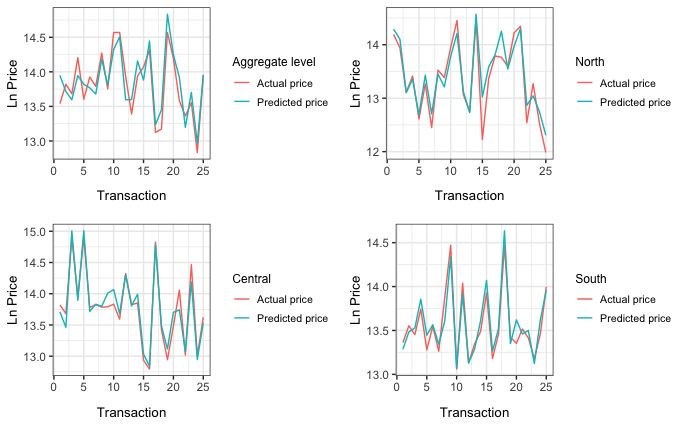
• Screening the collected data set, data cleansing, and applying imputation and
  winsorization methods.

• Detecting multicollinearity problem.

• Applying the hedonic price approach in the aggregate market level to develop
  property appraisal models and using White’s standard errors test in the
  presence of heteroskedasticity.

• Stratifying the housing market in the city of Boulder based on both prop-
  erty types and location to create a number of homogeneous submarkets and
  performing the hedonic models in different submarket levels.

    The rest of the paper is organized as follows. Section 2 provides an overview
of the literature that employs hedonic regression models. Following this, section
3 explains the empirical models, section 4 presents the data set and the variables,
and section 5 elaborates the methodologies used in this paper. The results
obtained from performing hedonic regression methods described in section 6.
Finally, conclusions and implications are provided in section 7.

2    Related Literature
    Hedonic price analysis originates from Waugh (1928), Court (1939), Stone
(1954), Adelman and Griliches (1961), and Lancaster (1966). Lancaster (1966)
states that “the good, per se, does not give utility to the consumer; it possesses
characteristics, and these characteristics give rise to utility”. For example a
house can be viewed as an aggregation of individual attributes such as (lot size,
number of bedrooms, bathrooms, and garages) which are implicitly embodied in
the house and its utility is generated by characteristics of the house.

    The hedonic regression model has numerous applications. Hedonic approaches
have been used to construct quality-adjusted price indexes for differentiated
goods. Namely, hedonic price model has been applied to estimate agricultural
commodities value (see e.g., Ethridge and Davis (1982) and Wilson (1984)).
Several studies have verified the ability of the hedonic regression model to ex-
plain the property rental prices determinants (see e.g., Zhang and Yi (2017),
and Gluszak and Zygmunt (2018)). Hedonic regression models have been used
to explain variations in dwelling prices and to determine the impact of specific
attributes on house prices. Many studies explored the influence of distance to
the central business district (CBD), employment centers, park, shopping center,
or school on housing values using hedonic housing price models. Examples of
these literature include Malpezzi et al. (1981), Adair et al. (2000), Söderberg
and Janssen (2001), Chin and Foong (2006), Ottensmann et al. (2008), Cao
and Hough (2012), and Tong and Gunter (2020). All found an overall declining
pattern of property values with distance from these locations. In addition, a

                                         2
number of studies have applied the hedonic price technique to quantify the effects
of environmental features like air, river, and noise pollution on house values (see
e.g., Anselin and Lozano-Gracia (2008), Mei et al. (2020), Chen (2017), Chang
and Kim (2013), and Bishop et al. (2020).

    Butler (1980) argues that the implicit assumption in hedonic price methods
is that all potential house buyers and suppliers interact in a single market and
the market can be characterised by a single hedonic equation determined by the
interaction of a supply and demand in a unitary market. However, the urban
housing markets are too compounded to be considered as homogeneous goods.
Some studies examined heteroscedasticity in hedonic house price models (see
e.g., Fletcher et al. (2000), Stevenson (2004), and Kestens et al. (2006)). The
evidence indicated the presence of heteroscedasticity.

    The heterogeneity of an urban property market gives rise to its likely seg-
mentation. Real estate market is spatial in nature and many property markets
may exist simultaneously within a single urban area. Day (2003) states the
property market is not a global or even a national market. It is argued that to
obtain unbiased estimates of the implicit prices identifying segmentation of the
property market is essential. Some studies, namely, Adair et al. (1996), Watkins
(2001), Berry et al. (2003), Lipscomb and Farmer (2005), Tu et al. (2007), Liu
et al. (2020), and Nishi et al. (2021) utilized hedonic price techniques to test
for market segmentation. They recognised the importance of both spatial and
structural characteristics when defining submarkets and observed greater levels
of homogeneity in the sample at a submarket level. They conclude that dividing
the market into the submarkets normally improves the predictive power of the
hedonic regression models.

   In this study we stratify the housing market in the city of Boulder into a
number of distinct submarkets to create a number of homogeneous submarkets
from the aggregate heterogeneous dwelling market based on both property types
and location.

3    Hedonic Price Model
    The hedonic housing price regression model is essentially a function of a
bundle of property characteristics such as structural attributes, socio-economic
status of the neighbourhood, environmental amenities, and location. The hedonic
housing price method is constructed by regressing the price of dwellings on a
vector of housing attributes. Various functional forms have been applied in
the literature to estimate the hedonic-price function including linear, semi-log,
log-log, quadratic, and Box-Cox transformations. Here, we estimate hedonic
price models for sold houses using a log-log specification. The advantage of
a log-log specification over other models is that the log transformation of the

                                        3
dependent variable (house price) often mitigates heteroskedasticity. The log
transformation reduces the problem of heteroskedasticity associated with the use
of the highly-skewed sales price variable. Figure 1 plots the distribution of house
prices before and after applying the log-transformation. Another important
advantage of the log-log model is in obtaining a constant elasticity. In a log-log
model the coefficients for those logarithmic terms are interpreted as elasticities.
For example, we do log transformation on the regressor “Living Area” to over-
come non-linearity problems. The estimated coefficient on “Ln(Living Area)”
measures the elasticity of property value with respect to the size of living area.
In a log-log model a coefficient on a dummy variable such as a swimming pool
that takes the value of 1 if the house has one and zero otherwise, represents on
average an approximate percentage difference in the prices of houses that have a
swimming pool compared to those that do not.

Figure 1: Distribution of House Prices before and after Applying the Log-
transformation.

   The hedonic model using a log-log specification for houses sold over a year
can be written as follows:

   Ln(P ) = Xβ +

where P is a [N × 1] vector and denotes house prices. X is a [N × K] matrix
of K independent variables describing the quantities of K characteristics of a
property’s structure, neighbourhood characteristics, and location.  is a [N × 1]
vector of random error terms and β is a corresponding [K × 1] vector of unknown
parameters named regression coefficients. By using an ordinary least squares

                                        4
estimation method (OLS), the regression coefficients are estimated as:
β̂ = (X T X)−1 X T Y
The price of any residential property is affected by many property factors,
namely, its structural, neighbourhood, and spatial attributes. Omitting impor-
tant attributes from the hedonic regression model might bias estimates of implicit
prices. To avoid misspecification biases a wide range of physical, neighborhood,
locational and accessibility factors are controlled in the above hedonic model
of residential property value. Here, to capture the structural attributes of the
properties features such as number of bedrooms, bathroom, parking, and HOA
fees (the annual fees for community costs) are included in our model. The
dummy variables are used to represent the presence or absence of particular
physical features and amenities such as a swimming pool, sauna, jacuzzi, or
tennis court. The value 1 indicates the presence of a swimming pool, jacuzzi, or
tennis court; a value of 0, represents otherwise. Other variables including house
value, size of the living area, and lot area, are defined in natural logarithmic
forms. The age of a property (in years) is computed from its date of completion
to the year sold. The relationship between price and age is not expected to be
linear. We are capturing the non-linear association between age and the house
price by adding a quadratic term for property age. To explore the influence
of propertie’s distance to the important amenities namely employment centers,
shopping centers, and schools we made use of Google Maps. For instance, to
measure the accessibility of the property to employment centers and shopping
centers we use driving time to the Boulder central business district (CBD) in
downtown measured in minutes. In addition, to measure the accessibility of a
house to the educational establishments we are adding the walking distance to
primary, middle, and high school measured in time (minutes). To include the
quality of the property’s neighborhood we are adding school ratings; primary
School, middle School, and high School Rates as well as the crime rate to our
model. In addition, we are entering the socio-economic variables such as median
household income and population density to our model.
4 Data
The data set we collected in this study to estimate the hedonic price model
consists of 1061 residential properties sold in the city of Boulder, Colorado. To
isolate the influence of time on property prices the data used in this study is
restricted to houses sold in a single year between January 1, 2019 and December
31, 2019 (see Eckert et al. (1990)). Samples used for hedonic estimation are
not necessarily random draws from the population of dwellings, but are recently
sold properties. Robinson (1979) states that “recent sales are not necessarily a
random draw from the total housing stock. If the purpose is to index the market
of available units, this may not be of great concern, but if the purpose is to index
5the total stock, we must concern ourselves with possible selection bias”. Several
studies have tested the existence of such biases. So far most studies have found
the magnitude of the bias to be modest (see e.g., Gatzlaff and Haurin (1998)).
We collected real estate datasets from different resources consisting of Multi-
ple Listing Service database1 , Public School Ratings2 , Colorado Crime Rates
and Statistics Information3 , CrimeReports4 , WalkScore5 , and US Census Bu-
reau6 . Before proceeding with the estimation of our models we merged all
data sets obtained from these websites. We screened our collected data set.
Among these transactions 4 houses were in rough shape and needed to be rebuilt.
Consequently, we deleted those 4 observations. All houses except one; which
has lots of luxury furniture, have been sold unfurnished. So, we dropped the
only furnished property. 30 properties were reported as horse properties. We
eliminated those associated records. We checked for duplicate records. We found
4 duplicate transactions and eliminated those. In a number of observations we
faced missing data points for some characteristics. For example, in some records
the information for variables “Bedroom”, “Full Bathroom”, “Parking”, “Lot Area”,
“HOA Fees”, “Solar Power” and “Pool, Bath tub, Sauna, or Jacuzzi” were missing.
We updated some of these missing data points by visiting different websites
and looking up for the correct information. Finally, a few observations left
with missing data points for the continuous variable “Lot Area” and the dummy
variables “Solar Power” and “Pool, Bath tub, Sauna, or Jacuzzi”. To deal with
missing data points we could eliminate from the model any attributes that have
missing values, or alternatively we could drop all those properties with missing
attributes. However, deleting observations due to an incomplete list of attributes
can cause sample size reduction and sample selection bias (see e.g., Hill (2013)).
Instead, to avoid losing the samples from analysis we imputed missing values
in the variable “Lot Area” with its mean. Similarly, we imputed missing values
for the dummy variables “Solar Power” and “Pool, Bath tub, Sauna, or Jacuzzi”
with their mode. Another problem we encountered is the presence of outliers.
The outliers were identified by calculating the 95% percentile. To mitigate the
influence of outliers on the analysis, we applied one-sided 95% or two-sided 90%
Winsorization. That means outliers were set to the value of the 95% percentile.
The data cleaning process left us with a final sample of 1018 observations. The
structural, spatial, and neighborhood attributes that are used in our analysis,
are summarized in Table 1 and 2. In addition to the mean, standard deviation,
minimum and maximum, information about the relative standard deviation (the
coefficient of variation (CV = σµ ), which represents the extent of variability in
relation to the average of the variable has been reported in Table 1.
1 https://realtyna.com/blog/list-mls-us
2 https://www.greatschools.org
3 https://www.neighborhoodscout.com/co/crime
4 https://www.cityprotect.com
5 https://www.walkscore.com
6 https://data.census.gov/cedsci
6Table 1: Descriptive Statistics for Numerical Variables.
Aggregate Level
Variables
Mean St. Dev. Min Max Coefficient of Variation (CV)
House Price ($) 896, 332 679,195.8 112,897 7,200,000 76%
Ln(House Price) 13.49 0.57 12.18 14.57 4%
Ln(Lot Area) (SqFt) 6.21 4.37 0.00 14.27 70%
(Ln(Lot Area))2 57.67 43.97 0.00 203.68 76%
Ln(Living Area) (SqFt) 7.54 0.61 6.03 9.25 8%
(Ln(Living Area))2 57.27 9.24 36.37 85.47 16%
Age (year) 43.12 21.46 1 98 50%
Age2 2,319.19 2,253.79 1 9,604 97%
Full Bathroom 1.55 0.76 0 3 49%
Half Bathroom 0.41 0.51 0 2 124%
4 Bathroom 0.64 0.69 0 2 108%
3
Parking 1.68 0.71 0 3 42%
HOA Fees (annually) ($) 1,693.32 2,033.16 0 7,113 120%
Drive to CBD (minute) 11.42 6.91 1 26 61%
Walk to E.School (minute) 21.37 17.31 2 68 81%
Walk to M.school (minute) 33.21 27.72 2 96 83%
Walk to H.school (minute) 46.94 32.92 4 122 70%
Married (%) 42.97 16.87 9.90 70.30 40%
Median Household Inc. ($) 61,137.44 20,891.56 19,985 96,406 34%
Neighborhood’s Population 43,641.85 46,872.42 888 99,081 107%
Sample size 1018
City of Boulder is divided into seven different geographical locations; central
Boulder, downtown Boulder, old north Boulder, north Boulder, south Boulder,
east Boulder, Gunbarel, and rural areas. Figure 2 plots the city of Boulder on
the map. With city development, the old north Boulder neighborhood is in
central Boulder. Therefore, we are merging the data for the central Boulder and
old north Boulder. We explored the geographical location of each property by
making use of Google Maps. For example, in the north Boulder region there
are 238 transactions. 200 dwellings sold in the east Boulder. There are only
49 transactions in downtown Boulder. Because the number of transactions in
downtown Boulder is limited we are merging the data for the central Boulder
and downtown Boulder. Finally, we are considering six different geographical
areas in the city of Boulder as central Boulder, north Boulder, south Boulder,
east Boulder, Gunbarel, and rural areas. Table A.5 in the appendix provides
more information about the number of transactions in different geographical
locations in 2019.
The property types in the housing market in the city of Boulder are classified
as condominiums, town-homes, and single-family houses. The town-home prop-
erties in the city of Boulder have been classified into the west of the Broadway
7Table 2: Descriptive Statistics for Categorical Variables.
Aggregate Level
Variables
Levels Description Frequency Percent
0 No 724 71.12
Pool, Bath tub, Sauna, or Jacuzzi 1 Yes 360 35.36
0 No 658 64.64
Solar Power 1 294 28.88 Yes
1 A 334 32.81
Nearest E.School Rank 2 B 548 53.83
3 C 136 13.36
1 A 125 12.28
Nearest M.School Rank 2 B 633 62.18
3 C 260 25.54
Nearest H.School Rank 1 A 1018 100
1 Central 230 22.59
2 North 238 23.38
3 South 143 14.05
Region 4 East 200 19.65
5 Gunbarrel 125 12.28
6 Rural 82 8.06
0 0 bedroom 3 0.29
1 1 bedroom 72 7.07
2 2 bedrooms 253 24.85
Number of Bedrooms 3 3 bedrooms 285 28.00
4 4 bedrooms 249 24.46
5 5 bedrooms 127 12.48
6 6 bedrooms 27 2.65
7 7 bedrooms 2 0.20
1 Condominum 324 31.83
Property Type 2 Town - Home 90 8.84
3 Single Family 604 59.33
1 Highest crime rate 82 8.06
Neighborhood’s Crime Level 2 Middle crime rate 505 49.61
3 Lowest crime rate 431 42.34
Sample size - 1018 100 -
8Figure 2: City of Boulder.
highway and downtown, and the east of the Broadway highway and all other
areas in the city of Boulder7 . There are only 22 town-homes to the west of
the Broadway highway and downtown and 69 town-homes to the east of the
Broadway highway and all other areas in the city of Boulder. Small number of
observations makes the creation of reliable and robust models difficult. Malpezzi
(2002) states that if sample sizes are small, it is normally best to avoid disaggre-
gating the market. Consequently, we are combining the sold town-homes to the
west and east of the Broadway highway and the downtown.
Before proceeding with our models we should test for multicollinearity prob-
lems, the common issue in hedonic regression models. In the presence of high
correlation the estimated coefficients may be unreliable (see e.g., Sheppard
(1999)). Due to high correlation, the corresponding coefficients might be esti-
mated as statistically insignificant when in fact they are statistically significant.
Consequently this problem poses an inaccurate interpretation of coefficients and
makes it difficult to recognize important regressors. To ensure the robustness of
our model, the Pearson correlation coefficient is computed. Figure 3 summarizes
this information. Positive correlations are shown in red color and negative
correlations in dark blue color. The color intensity and the size of the circle are
7 https://www.bouldercounty.org/property-and-land/assessor/sales/comps-2019/
residential
9Figure 3: Correlation Plot.
proportional to the correlation coefficients. We drop variables which generate
pairwise correlation coefficients greater (smaller) than the common thresholds
0.8 (-0.8). In the citywide housing market we observed that variables “Walk to
H.school”, “Drive to CBD”, “Married” and “Median Household Inc.” are highly
correlated. To avoid multicollinearity problems we dropped “Walk to H.school”
and “Married” and calculated the Pearson correlation coefficient one more time.
In addition, we calculated √
the generalized
√ variance inflation factors (GVIF). The
accepted GVIF cutoff is V IF = 5 = 2.24. In the aggregate level data set
no GVIF is above the defined thresholds. Therefore, we keep the rest of the
variables in the model.
5 Aggregate and Disaggregate Market Levels
We first estimate the hedonic price equation at the citywide market level;
over all 1018 houses sold in the city of Boulder in 2019. To control for property
type and location differences we are adding categorical variables into the hedonic
pricing model. We use a non-stepwise regression method and keep both statis-
10tically significant and non-statistically significant regressors in our regression
model. An underlying problem with stepwise regression is that in the presence
of heteroscedasticity, the results of the t-tests are unreliable. Consequently,
some regressors that have causal effects on the dependent variable may not be
statistically significant, although some other regressors may be significant by
chance. Therefore, using a stepwise regression method may fit the model well
over our sample (overfitting), but nonetheless, do poorly over an unseen data
set (see e.g., Smith (2018)). Initially, we are employing an ordinary least square
(OLS) estimation method to provide information of the attributes affecting the
housing market in Boulder, Colorado. Table 3 summarizes this information.
The urban property markets contain high variation in the structural, loca-
tional, neighbourhood, and environmental attributes. We both graphically and
statistically detected heteroskedasticity in the aggregate market level. In the
presence of heteroskedasticity OLS estimators are unbiased, while the standard
error and the statistics we used to test hypotheses based on ordinary least square
estimation method will be inefficient. Following Fletcher et al. (2000) we use
White’s standard errors test to correct the issue of incorrect standard errors
and test statistics. The robust standard errors and heteroskedasticity-consistent
estimates are reported in Table 4.
In the presence of heteroscedasticity a single model over the pooled property
data set is not reliable. A model over the aggregate housing data set is assessing
the whole city and would hold in high variation in houses characteristics. Less
difference in house attributes lead to a more homogeneous market which may
provide more efficient and reliable estimates. In the light of these facts, we
stratify the market into a number of distinct submarkets to create a number of
homogeneous submarkets from the aggregate heterogeneous dwelling data set.
Normally, a submarket composed of groups of relatively homogenous dwellings
that are recognised as close substitutes to potential house buyers (see e.g., Good-
man and Thibodeau (1998), Bourassa et al. (2003), Taylor (2008), Páez et al.
(2008), Wheeler et al. (2014), and Wu et al. (2020)). There is no consistent
definition for housing submarkets. Some researchers suggested that housing
submarkets compose of all houses with similar environmental characteristics.
Others have defined dwelling submarkets based on socio-economic attributes (see
e.g., Palm (1978)). Some analysts have defined dwelling submarkets based on
the structural characteristics (see e.g., Watkins (1999), Adair et al. (2000), and
Carriazo and Gomez-Mahecha (2018)). Others have defined dwelling submarkets
as a collection of houses within a specific location (see e.g., Straszheim (1975),
and Keskin and Watkins (2017)). Interestingly, some other researchers have
realized the importance of both structural and locational factors in determining
housing market segmentations (see e.g., Adair et al. (1996), Watkins (2001),
Alkana et al. (2015), Xiao et al. (2016), and Bello et al. (2020)).
To test for market segmentation we first stratify the housing market in the
city of Boulder based on both property type and location. Next, we nest housing
11Table 3: Hedonic Model Estimates
OLS Method.
Aggregate Level
Independent Variables
Coeff. Std. Error T-Statistics
(Intercept) 13.49 1.65 8.20∗∗∗
Ln(Lot Area) 0.38 0.06 5.79∗∗∗
(Ln(Lot Area)) 2
-0.004 0.003 -1.36
Ln(Living Area) -0.48 0.45 -1.08
(Ln(Living Area)) 2
0.07 0.03 2.30∗∗
Age -0.02 0.01 -3.95∗∗∗
Age2 0.0001 0.0000 7.39∗∗∗
Number of Bedrooms
(Bedrooms)2 0.06 0.04 1.73∗
(Bedrooms)3 0.02 0.05 0.52
(Bedrooms)4 -0.02 0.05 -0.46
(Bedrooms)5+ -0.05 0.06 -0.96
Full Bathroom 0.08 0.02 4.69∗∗∗
Half Bathroom 0.01 0.02 0.85
3
4 Bathroom 0.06 0.02 3.54∗∗∗
Parking 0.04 0.01 3.12∗∗
HOA Fees 0.0000 0.0000 1.74∗
School Ranking
(Nearest E.School Rank)2 -0.06 0.02 -2.84∗∗∗
(Nearest E.School Rank)3 -0.17 0.03 -5.04∗∗∗
(Nearest M.School Rank)2 -0.18 0.04 -4.06∗∗∗
(Nearest M.School Rank)3 -0.14 0.05 -2.76∗∗∗
(Pool, Bath tub, Sauna, or Jacuzzi)1 0.04 0.02 2.21∗∗
(Solar Power)1 0.09 0.03 3.17∗∗∗
Drive to CBD -0.02 0.003 -7.32∗∗∗
Walk to E.School -0.0003 0.001 -0.48
Walk to M.school -0.001 0.001 -1.45
Median Household Inc. -0.0000 0.0000 -0.62
Neighborhood’s Population -0.0000 0.0000 -1.21
12Table 3: (Continued.)
Aggregate Level
Independent Variables
Coeff. Std. Error T-Statistics
Crime Levels (Base: Level 3)
Neighborhood’s Crime Level: 1 -0.09 0.03 -2.61∗∗∗
Neighborhood’s Crime Level: 2 -0.03 0.02 -1.70∗
Property Type
Single Family Houses -1.05 0.24 -4.35∗∗∗
Town-Home Houses -1.10 0.23 -4.84∗∗∗
Regions (Base: Central)
(North)2 -0.16 0.03 -4.88∗∗∗
(South)3 -0.14 0.05 -3.00∗∗∗
(East)4 -0.22 0.04 -6.26∗∗∗
(Gunbarrel)5 -0.18 0.06 -3.01∗∗∗
(Rural)6 -0.30 0.06 -4.94∗∗∗
Ln(Lot Area):Ln(Living Area) -0.02 0.01 -3.70∗∗∗
Ln(Living Area):Age 0.001 0.001 2.01∗∗
Sample size 1018
R 2
0.865
Adj. R 2
0.86
F-statistic (p−value) 169.7 (0.000)
Dependent variable: Ln(Price)
Note: ∗ ∗ ∗, ∗ ∗, and ∗ indicate p < 0.01, p < 0.05, and p < 0.1 respectively.
Base group in the citywide housing market: condominium houses, with one
bedroom or less, no pool, bath tub, sauna, or jacuzzi, no solar power, in the
central Boulder region with crime level 3.
13Table 4: Hedonic Model Estimates
White Correction.
Aggregate Level
Independent Variables
Coeff. White’s Std. Error White’s T-Statistics
(Intercept) 13.49 1.62 8.32∗∗∗
Ln(Lot Area) 0.38 0.10 3.78∗∗∗
(Ln(Lot Area)) 2
-0.004 0.005 -0.85
Ln(Living Area) -0.48 0.44 -1.10
(Ln(Living Area)) 2
0.07 0.03 2.34∗∗
Age -0.02 0.01 -3.00∗∗∗
Age 2
0.0001 0.0000 5.73∗∗∗
Number of Bedrooms
(Bedrooms)2 0.06 0.04 1.71∗
(Bedrooms)3 0.02 0.05 0.49
(Bedrooms)4 -0.02 0.06 -0.44
(Bedrooms)5+ -0.05 0.06 -0.89
Full Bathroom 0.08 0.02 4.68∗∗∗
Half Bathroom 0.01 0.02 0.80
3
4 Bathroom 0.06 0.01 3.76∗∗∗
Parking 0.04 0.01 2.74∗∗∗
HOA Fees 0.0000 0.0000 1.38
School Ranking
(Nearest E.School Rank)2 -0.06 0.02 -2.67∗∗∗
(Nearest E.School Rank)3 -0.17 0.03 -5.27∗∗∗
(Nearest M.School Rank)2 -0.18 0.04 -4.35∗∗∗
(Nearest M.School Rank)3 -0.14 0.05 -2.83∗∗∗
(Pool, Bath tub, Sauna, or Jacuzzi)1 0.04 0.02 2.08∗∗
(Solar Power)1 0.09 0.03 2.46∗∗
Drive to CBD -0.02 0.003 -5.94∗∗∗
Walk to E.School -0.0003 0.001 -0.47
Walk to M.school -0.001 0.001 -1.22
Median Household Inc. -0.0000 0.0000 -0.53
Neighborhood’s Population -0.0000 0.0000 -1.08
submarkets based on property type within spatially defined housing market
segmentation.
To avoid violating the classical linear model assumptions we estimate the
hedonic price regression model for each submarket separately using the OLS
14Table 4: (Continued.)
Aggregate Level
Independent Variables
Coeff. White’s Std. Error White’s T-Statistics
Crime Levels (Base: Level 3)
Neighborhood’s Crime Level: 1 -0.09 0.03 -2.65∗∗∗
Neighborhood’s Crime Level: 2 -0.03 0.02 -1.61
Property Type
Single Family Houses -1.10 0.41 -2.68∗∗∗
Town-Home Houses -1.05 0.43 -2.45∗∗
Regions (Base: Central)
(North)2 -0.16 0.04 -4.36∗∗∗
(South)3 -0.14 0.05 -3.02∗∗∗
(East)4 -0.22 0.04 -5.48∗∗∗
(Gunbarrel)5 -0.18 0.07 -2.55∗∗
(Rural)6 -0.30 0.07 -4.33∗∗∗
Ln(Lot Area):Ln(Living Area) -0.02 0.01 -3.37∗∗∗
Ln(Living Area):Age 0.001 0.001 1.65∗
Chi-squared (p−value) 115 (0.002)
Dependent variable: Ln(Price)
Note: ∗ ∗ ∗, ∗ ∗, and ∗ indicate p < 0.01, p < 0.05, and p < 0.1 respectively.
estimation methods. In the submarkets based on property type to control for
location differences categorical variables are added into the hedonic pricing
models. Similarly, in the submarkets based on spatial attributes to control for
property type differences categorical variables are included into the hedonic
pricing models. In a number of submarkets due to the limited number of houses,
some of the categorical variables were removed.
Next, we perform Chow test to examine if there is significant difference
between hedonic price regression models across distinct submarkets (see e.g.,
Watkins (1999), Yu (2006), Taylor (2008), Gavu and Owusu-Ansah (2019), and
Yang et al. (2020)).
Finally, we nest structural submarkets within spatial submarkets and focus
on the joint importance of both structural and locational attributes in classifying
submarkets.
156 Results
In this section we first provide summary statistics about the houses in the
aggregate level. Among the 1018 residential properties sold during 2019 in the
city of Boulder, the asset prices range between $112, 897 and $7, 200, 000, with an
average price of $896, 332 and a median price of $729, 500. The average “Living
Area” and “Lot Area” are 2, 264 and 18, 367 square feet respectively. The average
age of the dwellings is approximately 43 years old. In this data set the houses
have 3.16 bedrooms on average with 0.29% of them having no bedroom and
15.32% of them having 5 bedrooms or more. Moreover, 28.88% of the dwellings
have solar power and 35.36% of them have a pool, bath tub, sauna, or jacuzzi.
More information about the descriptive statistics of the variables in the citywide
housing market level can be found in Table 1 and 2.
Next, we bring descriptive statistics about the houses in the disaggregate
level. Amongst the 1018 dwellings in our data set, 604 are single family houses,
324 are condominiums, and 90 are town-homes. The single family property prices
range between $216, 575 and $7, 200, 000, with an average price of $1, 160, 321.
In the town-home submarket the house prices range between $115, 000 and
$1, 421, 000, with an average price of $627, 960. In the condominium submarket
the dwelling prices range between $112, 897 and $2, 600, 000, with an average
price of $478, 751. In the single family housing submarket the dwellings have
3.82 bedrooms on average with 0.17% of them having no bedroom and 24.51%
of them having 5 bedrooms or more. The houses in the town-home submarket
have 2.97 bedrooms on average with 7.78% of them having 5 bedrooms or more.
In the condominium submarket the houses have 1.98 bedrooms on average with
0.62% of them having no bedroom and 0.31% of them having 5 bedrooms or
more. In the single family housing submarket 3.31% of the houses have solar
power and 18.05% of the houses have a pool, bath tub, sauna, or jacuzzi. We do
not have much information about the existence of solar power, pool, bath tub,
sauna, or jacuzzi in the town-home or condominium submarkets.
In the locational submarkets the average age of the dwellings are almost
30 years old in north Boulder, 59 years old in central Boulder, 53 years old in
south Boulder, 40 years old in east Boulder, 37 years old in Gunbarrel, and 41
years old in the rural region. In addition, in the spatial submarkets, namely,
north Boulder region with 238 transactions the house prices range between
$134, 306 and $4, 500, 000, with an average price of $807, 214. Amongst the 230
dwellings sold in the central Boulder the house values range between $115, 000
and $7, 200, 000, with an average price of $1, 256, 235. Table A.5 in the appendix
provides more information about the descriptive statistics of the house prices in
different submarkets. From Table A.5 we learn that the deviation in residential
property prices is lower in the north, south, east, Gunbarrel submarkets, than
the aggregate market level. However, the house price difference is higher in
central Boulder and rural areas.
16Given the descriptive statistics of the houses attributes we will now focus on
the outcomes from performing the hedonic models in different submarket levels.
Initially, to ensure the robustness of our models at the disaggregate levels, the
Pearson correlation coefficients have been computed in each submarket. Namely,
in the central Boulder submarket the variables “HOA Fees” and “Ln(Living
Area)” are greatly correlated (0.88). In south Boulder, VIF for the regressors
“Median Household Inc.” and “HOA Fees” is 16.27 and 8.20 respectively. Vari-
ables “Ln(Lot Area)” and “Ln(Living Area)” are highly correlated in Gunbarrel
(0.83). In addition, the correlation between variables “Drive to CBD” and “Walk
to E.School” is 0.81. In the rural submarket the correlation between “Walk
to E.School” and “Walk to M.School” is 0.91. In consideration of these high
correlations, to prevent multicollinearity problems we excluded these explanatory
variables from the hedonic models in these submarkets.
Based on the outcomes from the hedonic models in different submarkets,
we observe that the estimated marginal contribution of the residential property
features on house values vary. However, in general, the sign of the marginal
effect of the dwellings’ characteristics are consistent with our expectations. For
instance, as anticipated the higher the size of the lot area the higher the house
prices are or the existence of solar power significantly raises the house value.
Age of the property is negatively associated with the dwelling value, but the
age-squared term is positively related to the house price. Moreover, commuting
time to the CBD negatively impacts the property prices. Allocation of the
dwellings in the neighborhoods with lower crime rate add to their values except
in Gunbarrel and south Boulder. Additionally, the presence of a swimming pool,
sauna, or jacuzzi add to the dwelling values. For more details see Table A.6 and
A.7 in the appendix.
To compare the explanatory power of the hedonic regression models at the
aggregate and disaggregate levels we rely on values of adjusted R2 which are
ranged from 0.73 to 0.91. The values of adjusted R2 from the models in the struc-
tural submarkets are smaller than the model in the citywide level. This could
be due to smaller sample sizes and fewer regressors in the models. Nevertheless,
in the spatial submarkets the models in all submarkets, but rural submarket,
have higher adjusted R2 and higher explanatory powers than the model in the
citywide level. The higher levels of explanation in the spatial submarkets might
represent the importance of locational characteristics in determining housing
market segmentations in the city of Boulder. More information about the ex-
planatory power of these models can be learned from the bar-plots in Figure 4.
In addition to measuring the explanatory power of the hedonic regression
models, we checked for the homogeneity assumption in different models. We
observed a higher level of homogeneity in most housing submarkets compared
to the citywide housing market level. The p-value from the Breusch-Pagan test
is represented in Table A.8. Moreover, to evaluate the performance of hedonic
17Figure 4: Comparison of the Performance of Hedonic Regression Models in
Different Submarkets.
models over different market levels, we computed the performance metric, the
mean squared error (MSE). The values of the MSE are lower for all submarkets
except central Boulder and rural submarkets. Given the level of homogeneity in
the housing submarkets and also the house price variability these outcomes have
been expected. The values of MSE in the aggregate and disaggregate levels, are
depicted in Figure 5.
Furthermore, to visualize the accuracy of our housing price prediction models
we plotted dwellings’ actual and predicted prices in the aggregate and disaggre-
gate levels (Figure 6 and 7).
To examine if there are significant differences between hedonic models across
distinct segments we performed Chow test. The results from Chow test are
presented in table A.9 in the appendix. These results indicate that significant
structural differences exist between single family and condominium submarkets.
Similarly, we observe significant structural differences across single family and
town-home segments. Nonetheless, the results from the chow test implies no
sufficient evidence of market segmentation between town-home and condominium
submarkets. Considering this, we merged these two submarkets and considered
them as a single homogeneous market (condo-town-home).
18Figure 5: Comparison of the Mean Squared Errors in Different Submarket Levels
with the Citywide Market Level.
Furthermore, the results from chow test, shown in table A.10 in the appendix
confirms that spatial differences exist across most of the submarkets. For in-
stance, the central Boulder differs from all other submarkets at 1% significance
level. The north and south Boulder submarkets vary from east Boulder. The east
Boulder submarket differs from Gunbarrel. For those special submarkets that
indicate no significant house price differences such as north and the rural area,
south and Gunbarrel we combined these submarkets and named this merged
submarket, north south Gunbarrel rural (NSGR) submarket.
Finally, we nested structural housing submarkets within spatial housing seg-
mentations. We observed that in the nested single family home submarket within
the NSGR submarket (NSGR-single family) the variables “Walk to M.school”
and “Drive to CBD” are highly correlated (0.83). The variable “HOA Fees” is
also highly correlated with “Ln(Lot Area)” (0.81). In the nested central Boulder
submarket within the condo-town-home submarket (central-condo-town-home),
GVIF for the regressor “Neighborhood’s Crime Level” is 2.49. In the nested east
and condo-town-home submarket variables “Walk to M.school” and “Drive to
CBD” are highly correlated (-0.94). In addition, the GVIF for the categorical
variable “Nearest E.School Rank” is 3.83. In the nested NSGR and condo-town-
home submarket GVIF for variable “Nearest E.School Rank” is 3.13. In the
nested NSGR and single family housing submarket GVIF for the categorical vari-
1920
Figure 6: The Predicted Prices Obtained by Hedonic Regression Model in Structural Submarket and the Actual Prices.21
Figure 7: The Predicted Prices Obtained by Hedonic Regression Model in Spatial Submarket and the Actual Prices.22
Figure 7: (Continued) - The Predicted Prices Obtained by Hedonic Regression Model in Spatial Submarket and the Actual
Prices.able “Nearest M.School Rank” is 3.26. Consequently, to prevent multicollinearity
problems we excluded these explanatory variables from the hedonic models in
these nested submarkets. Table A.11 in the appendix represents a summary of
results for the hedonic models in different nested submarkets. Furthermore, we
compared hedonic price regression models for different nested submarkets us-
ing Chow test. Table A.12 in the appendix provides us with a summary of results.
7 Conclusion
In this paper we implemented hedonic price regression models, to predict
house prices in the city of Boulder, Colorado. In the urban property markets the
houses have heterogeneous characteristics. They differ in structural, locational,
neighbourhood, and environmental attributes. Consequently, in urban housing
markets stratification could improve the performance of housing price prediction
models. In this study, we stratified the real estate market in the city of Boulder
into the structural and spatial submarkets.
We compared several performance measurements for the predictions of the
house prices in the aggregate and disaggregate market levels. We observe higher
levels of homogeneity and explanatory power and lower values of the MSE in
most housing submarkets compared to the citywide housing market. In addition,
the results obtained from the Chow tests confirm the structural and spatial
differences across most of the submarkets. Considering these performance metrics
we are anticipating that the housing market in the city of Boulder should be
necessarily classified into the structural and spatial submarkets.
The hedonic models have great advantages. One major supremacy of the
hedonic model is its simplicity in interpreting the estimated parameters. Another
advantage of the hedonic methods is that the marginal values of the attributes
can be obtained by differentiating the price function with respect to each char-
acteristic (see e.g., McMillan et al. (1980)). Despite these advantages, hedonic
models have been mainly applied on the residential real estate market and
barely been implemented in other real estate markets. It would be interesting
to perform hedonic models over non-residential real estate markets, including
business, industrial, or commercial properties such as hotels, clubs, educational
properties, hospitals, and farms.
In addition, it would be interesting to compare the performance of the hedo-
nic approach with the machine learning and deep learning algorithms such as
artificial neural network, random forest, k nearest neighbor, and support vector
regression which have been offered for the house price valuation and real estate
property price prediction model.
23Acknowledgements
Thanks goes to Dr. Nicholas E. Flores8 for his comments.
8 Department Chair of Economics, Colorado University at Boulder
24References
Adair, A., McGreal, S., Smyth, A., Cooper, J., and Ryley, T. (2000). House
prices and accessibility: The testing of relationships within the belfast urban
area. Housing studies, 15(5):699–716.
Adair, A. S., Berry, J. N., and McGreal, W. S. (1996). Hedonic modelling,
housing submarkets and residential valuation. Journal of property Research,
13(1):67–83.
Adelman, I. and Griliches, Z. (1961). On an index of quality change. Journal of
the American Statistical Association, 56(295):535–548.
Alkana, L. et al. (2015). Housing market differentiation: the cases of yenima-
halle and çankaya in ankara. International Journal of Strategic Property
Management, 19(1):13–26.
Anselin, L. and Lozano-Gracia, N. (2008). Errors in variables and spatial effects
in hedonic house price models of ambient air quality. Empirical economics,
34(1):5–34.
Arvanitidis, P. A. (2014). The economics of urban property markets: an institu-
tional economics analysis. Routledge.
Bello, M. Z., Sanni, M. L., Mohammed, J. K., et al. (2020). Conventional
methods in housing market analysis: A review of literature. Baltic Journal of
Real Estate Economics and Construction Management, 8(1):227–241.
Berry, J., McGreal, S., Stevenson, S., Young, J., and Webb, J. (2003). Estimation
of apartment submarkets in dublin, ireland. Journal of Real Estate Research,
25(2):159–170.
Bishop, K. C., Kuminoff, N. V., Banzhaf, H. S., Boyle, K. J., von Gravenitz, K.,
Pope, J. C., Smith, V. K., and Timmins, C. D. (2020). Best practices for using
hedonic property value models to measure willingness to pay for environmental
quality. Review of Environmental Economics and Policy, 14(2):260–281.
Blomquist, G. and Worley, L. (1981). Hedonic prices, demands for urban housing
amenities, and benefit estimates. Journal of Urban Economics, 9(2):212–221.
Bourassa, S. C., Hoesli, M., and Peng, V. S. (2003). Do housing submarkets
really matter? Journal of Housing Economics, 12(1):12–28.
Butler, R. V. (1980). Cross-sectional variation in the hedonic relationship for
urban housing markets. Journal of Regional Science, 20(4):439–453.
Cao, X. and Hough, J. A. (2012). Hedonic value of transit accessibility: An
empirical analysis in a small urban area. In Journal of the Transportation
Research Forum, volume 47.
25Carriazo, F. and Gomez-Mahecha, J. A. (2018). The demand for air quality:
evidence from the housing market in bogotá, colombia. Environment and
Development Economics, 23(2):121–138.
Chang, J. S. and Kim, D.-J. (2013). Hedonic estimates of rail noise in seoul.
Transportation Research Part D: Transport and Environment, 19:1–4.
Chen, W. Y. (2017). Environmental externalities of urban river pollution and
restoration: A hedonic analysis in guangzhou (china). Landscape and Urban
Planning, 157:170–179.
Chin, H. C. and Foong, K. W. (2006). Influence of school accessibility on housing
values. Journal of urban planning and development, 132(3):120–129.
Court, A. (1939). Hedonic price indexes with automotive examples.
Day, B. (2003). Submarket identification in property markets: A hedonic housing
price model for glasgow. CSERGE Working Paper EDM.
Del Giudice, V., Manganelli, B., and De Paola, P. (2017). Hedonic analysis of
housing sales prices with semiparametric methods. International Journal of
Agricultural and Environmental Information Systems (IJAEIS), 8(2):65–77.
Eckert, J. K., Gloudemans, R. J., and Almy, R. R. (1990). Property appraisal
and assessment administration. International Assn of Assessing Office.
Ethridge, D. E. and Davis, B. (1982). Hedonic price estimation for commodities:
an application to cotton. Western Journal of Agricultural Economics, pages
293–300.
Fan, C., Cui, Z., and Zhong, X. (2018). House prices prediction with machine
learning algorithms. In Proceedings of the 2018 10th International Conference
on Machine Learning and Computing, pages 6–10.
Fletcher, M., Gallimore, P., and Mangan, J. (2000). Heteroscedasticity in hedonic
house price models. Journal of Property Research, 17(2):93–108.
Frew, J. and Jud, G. (2003). Estimating the value of apartment buildings.
Journal of Real Estate Research, 25(1):77–86.
Gatzlaff, D. H. and Haurin, D. R. (1998). Sample selection and biases in local
house value indices. Journal of Urban Economics, 43(2):199–222.
Gavu, E. K. and Owusu-Ansah, A. (2019). Empirical analysis of residential
submarket conceptualisation in ghana. International Journal of Housing
Markets and Analysis.
Gluszak, M. and Zygmunt, R. (2018). Development density, administrative
decisions, and land values: An empirical investigation. Land Use Policy,
70:153–161.
26Goodman, A. C. and Thibodeau, T. G. (1998). Housing market segmentation.
Journal of housing economics, 7(2):121–143.
Haase, D., Piorr, A., Schwarz, N., Rickebusch, S., Kroll, F., van Delden, H.,
Zuin, A., Taylor, T., Boeri, M., Zasada, I., et al. (2013). Tools for modelling
and assessing peri-urban land use futures. In Peri-urban futures: Scenarios
and models for land use change in Europe, pages 69–88. Springer.
Hill, R. J. (2013). Hedonic price indexes for residential housing: A survey,
evaluation and taxonomy. Journal of economic surveys, 27(5):879–914.
Jiang, L., Phillips, P. C., and Yu, J. (2014). A new hedonic regression for real
estate prices applied to the singapore residential market.
Keskin, B. and Watkins, C. (2017). Defining spatial housing submarkets: Explor-
ing the case for expert delineated boundaries. Urban Studies, 54(6):1446–1462.
Kestens, Y., Thériault, M., and Des Rosiers, F. (2006). Heterogeneity in hedonic
modelling of house prices: looking at buyers’ household profiles. Journal of
Geographical Systems, 8(1):61–96.
Król, A. (2020). The Application of Hedonic Methods in Quality-Adjusted Price
Indices. Wydawnictwo Uniwersytetu Ekonomicznego we Wrocławiu.
Lancaster, K. J. (1966). A new approach to consumer theory. Journal of political
economy, 74(2):132–157.
Lipscomb, C. A. and Farmer, M. C. (2005). Household diversity and market
segmentation within a single neighborhood. The Annals of Regional Science,
39(4):791–810.
Liu, Z., Cao, J., Xie, R., Yang, J., and Wang, Q. (2020). Modeling submarket
effect for real estate hedonic valuation: A probabilistic approach. IEEE
Transactions on Knowledge and Data Engineering, 33(7):2943–2955.
Malpezzi, S. (2002). Hedonic pricing models: a selective and applied review.
Housing economics and public policy, pages 67–89.
Malpezzi, S. et al. (1981). The flight to the suburbs: Insights gained from an
analysis of central-city vs suburban housing costs. Journal of Urban Economics,
9(3):381–398.
McMillan, M. L., Reid, B. G., and Gillen, D. W. (1980). An extension of
the hedonic approach for estimating the value of quiet. Land economics,
56(3):315–328.
Mei, Y., Gao, L., Zhang, J., and Wang, J. (2020). Valuing urban air quality: a
hedonic price analysis in beijing, china. Environmental Science and Pollution
Research, 27(2):1373–1385.
27Milon, J. W., Gressel, J., and Mulkey, D. (1984). Hedonic amenity valuation
and functional form specification. Land Economics, 60(4):378–387.
Nishi, H., Asami, Y., and Shimizu, C. (2021). The illusion of a hedonic price
function: Nonparametric interpretable segmentation for hedonic inference.
Journal of Housing Economics, 52:101764.
Ottensmann, J. R., Payton, S., and Man, J. (2008). Urban location and housing
prices within a hedonic model. Journal of Regional Analysis and Policy,
38(1100-2016-89822).
Páez, A., Long, F., and Farber, S. (2008). Moving window approaches for hedonic
price estimation: an empirical comparison of modelling techniques. Urban
Studies, 45(8):1565–1581.
Palm, R. (1978). Spatial segmentation of the urban housing market. Economic
Geography, 54(3):210–221.
Robinson, R. (1979). Housing economics and public policy. Springer.
Rosen, S. (1974). Hedonic prices and implicit markets: product differentiation
in pure competition. Journal of political economy, 82(1):34–55.
Sheppard, S. (1999). Hedonic analysis of housing markets. Handbook of regional
and urban economics, 3:1595–1635.
Smith, G. (2018). Step away from stepwise. Journal of Big Data, 5(1):32.
Söderberg, B. and Janssen, C. (2001). Estimating distance gradients for apart-
ment properties. Urban Studies, 38(1):61–79.
Stevenson, S. (2004). New empirical evidence on heteroscedasticity in hedonic
housing models. Journal of Housing Economics, 13(2):136–153.
Stone, R. (1954). The measurement of consumer behavior and expenditure in the
united kingdom, 1920-1938. Studies in the National Income and Expenditure
of the United Kingdom, 1.
Straszheim, M. R. (1975). Front matter," an econometric analysis of the urban
housing market". In An Econometric Analysis of the Urban Housing Market,
pages 16–0. NBER.
Taylor, L. O. (2008). Theoretical foundations and empirical developments in
hedonic modeling. In Hedonic methods in housing markets, pages 15–37.
Springer.
Tong, B. and Gunter, U. (2020). Hedonic pricing and the sharing economy:
How profile characteristics affect airbnb accommodation prices in barcelona,
madrid, and seville. Current Issues in Tourism, pages 1–20.
28Tu, Y., Sun, H., and Yu, S.-M. (2007). Spatial autocorrelations and urban housing
market segmentation. The Journal of Real Estate Finance and Economics,
34(3):385–406.
Waltl, S. R. (2018). Estimating quantile-specific rental yields for residential
housing in sydney. Regional Science and Urban Economics, 68:204–225.
Watkins, C. (1999). Property valuation and the structure of urban housing
markets. Journal of Property Investment & Finance.
Watkins, C. A. (2001). The definition and identification of housing submarkets.
Environment and Planning A, 33(12):2235–2253.
Waugh, F. V. (1928). Quality factors influencing vegetable prices. Journal of
farm economics, 10(2):185–196.
Wheeler, D. C., Paez, A., Spinney, J., and Waller, L. A. (2014). A bayesian
approach to hedonic price analysis. Papers in Regional Science, 93(3):663–683.
Wilson, W. W. (1984). Hedonic prices in the malting barley market. Western
Journal of Agricultural Economics, pages 29–40.
Wu, Y., Wei, Y. D., and Li, H. (2020). Analyzing spatial heterogeneity of housing
prices using large datasets. Applied Spatial Analysis and Policy, 13(1):223–256.
Xiao, Y., Orford, S., and Webster, C. J. (2016). Urban configuration, accessibility,
and property prices: A case study of cardiff, wales. Environment and Planning
B: Planning and Design, 43(1):108–129.
Yang, L., Chen, Y., Xu, N., Zhao, R., Chau, K., and Hong, S. (2020). Place-
varying impacts of urban rail transit on property prices in shenzhen, china:
Insights for value capture. Sustainable Cities and Society, 58:102140.
Yu, K. (2006). Studies in hedonic resale housing price indexes*.
Zhang, L. and Yi, Y. (2017). Quantile house price indices in beijing. Regional
Science and Urban Economics, 63:85–96.
29You can also read