Global Ecology and Conservation - SILVIS Lab
←
→
Page content transcription
If your browser does not render page correctly, please read the page content below
Global Ecology and Conservation 29 (2021) e01718
Contents lists available at ScienceDirect
Global Ecology and Conservation
journal homepage: www.elsevier.com/locate/gecco
Habitat connectivity for endangered Indochinese tigers
in Thailand
Naparat Suttidate a, b, Robert Steinmetz c, Antony J. Lynam d,
Ronglarp Sukmasuang e, Dusit Ngoprasert f, Wanlop Chutipong g,
Brooke L. Bateman a, Kate E. Jenks g, Megan Baker-Whatton g, Shumpei Kitamura h,
Elżbieta Ziółkowska i, Volker C. Radeloff a, *
a
SILVIS Lab, Department of Forest and Wildlife Ecology, University of Wisconsin-Madison, 1630 Linden Drive, Madison, WI 53706, USA
b
Department of Biology, Walailak University, 222 Thaibusi, Thasala, Nakhon Si Thammarat 80161, Thailand
c
World Wild Fund for Nature, 87 Phaholyothin 5, Samsen Nai, Phayathai, Bangkok 10400, Thailand
d
Wildlife Conservation Society, Global Conservation Program, 2300 Southern Boulevard, Bronx, NY 10540, USA
e
Department of Forest Biology, Faculty of Forestry, Kasetsart University, 50 Ngamwongwan Road, ChatuChak, Bangkok 10900, Thailand
f
Conservation Ecology Program, King Mongkut’s University of Technology Thonburi, 49 Soi Tientalay 25, Bangkhuntien-Chaitalay Road, Thakham,
Bangkhuntien, Bangkok 10150, Thailand
g
The Nature Conservancy, 4245 Fairfax Drive, Arlington, VA 22203, USA
h
Department of Environmental Science, Faculty of Bioresources and Environmental Sciences Ishikawa Prefectural University, 1-308, Suematu,
Nonoichi, Ishikawa 921-8836, Japan
i
Insitute of Environmental Sciences, Jagiellonian University in Kraków, Gronostajowa 7, 30-387 Kraków
A R T I C L E I N F O A B S T R A C T
Keywords: Habitat connectivity is crucial for the conservation of species restricted to fragmented populations
Carnivores within human-dominated landscapes. However, identifying habitat connectivity for apex preda
Circuit theory tors is challenging because trophic interactions between primary productivity and prey species
Dispersal corridor
influence both the distribution of habitats, and predator movement. Our goal was to assess habitat
Dynamic habitat indices
Graph theory
connectivity for Indochinese tigers (Panthera tigris) in Thailand. We quantified suitable habitat
Mammal conservation and dispersal corridors based an ensemble species distribution model that included prey distri
MODIS fPAR satellite data butions, primary productivity, and abiotic variables and was based on camera-trap data from
1996 to 2013 in 15 protected areas. We employed graph theory to evaluate the relative impor
tance of habitat patches and dispersal corridors to the overall connectivity network. We found
that tiger occurrence models with and without prey distributions performed well (Area Under the
Curve: 0.932–0.954). However, inclusion of prey distributions significantly improved model
performance (P < 0.001). Protected areas with tigers at the time of our surveys were highly
isolated with high resistance to movement within the dispersal corridors, and four of them have
lost their tiger populations since. Potential habitat patches outside of protected areas were also
mostly isolated, but it was encouraging to find that there is ample potential habitat that tigers are
not occupying. The Huai Kha Kaeng - ThungYai habitat patch and Kaeng Krachan dispersal
corridor were the most important for overall habitat connectivity. Generally, integrating prey
distributions into assessments of connectivity is a promising approach that can be widely applied
* Corresponding author.
E-mail address: radeloff@wisc.edu (V.C. Radeloff).
https://doi.org/10.1016/j.gecco.2021.e01718
Received 21 November 2020; Received in revised form 19 June 2021; Accepted 3 July 2021
Available online 5 July 2021
2351-9894/© 2021 The Authors. Published by Elsevier B.V. This is an open access article under the CC BY-NC-ND license
(http://creativecommons.org/licenses/by-nc-nd/4.0/).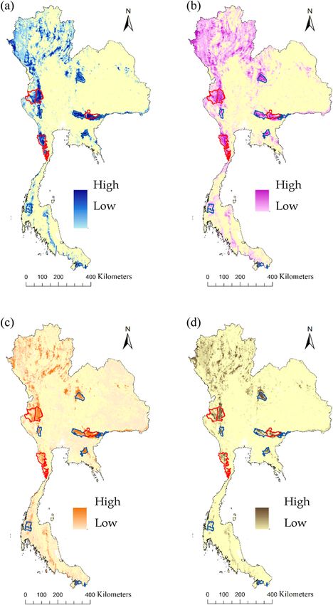
N. Suttidate et al. Global Ecology and Conservation 29 (2021) e01718
to predict species occurrence and delineate dispersal corridors, thereby supporting conservation
planning of tigers and other large carnivores.
1. Introduction
The loss and fragmentation of habitat poses an imminent threat to the viability of many species (Breckheimer et al., 2014; Hanski
and Triantis, 2015). Survival of species with fragmented habitat depends upon maintaining connectivity between isolated populations
(Hanski and Triantis, 2015; Carvajal et al., 2018). Landscape connectivity is defined as the degree to which a landscape facilitates or
impedes individual dispersal among habitat patches (Taylor et al., 1993), and connectivity can mitigate effects of climate change by
allowing species to track their fundamental niches (Hannah, 2011; Hamilton et al., 2018; Dickson et al., 2019). Therefore, connectivity
plays a crucial role in conservation planning where the goal is to preserve resilient habitat networks and design corridors that connect
remnant patches or protected areas (Rathore et al., 2012). However, models identifying habitat connectivity networks typically focus
on a single species, and do not capture species interactions such as competition and trophic interactions (Beier et al., 2011; Dutta et al.,
2018).
Trophic interactions shape the realized niche thereby affecting movement and dispersal success, and hence affect functional habitat
connectivity (Hebblewhite et al., 2014; Zarnetske et al., 2017). Carnivores require sufficient densities of prey, and herbivores need
plant resources (Bateman et al., 2012; Wisz et al., 2013). Thus, the distributions and abundance of species depends on both prey
distributions and abiotic factors, and both affect how species respond to landscape heterogeneity, and where dispersal corridors are
located (Araújo and Luoto, 2007; Guisan et al., 2013). However, studies of habitat connectivity for carnivores tend to focus only on
abiotic factors due to a paucity of data on prey abundance and occurrence, such as studies for jaguar (Panthera onca) (Rabinowitz and
Zeller, 2010; Ramirez-Reyes et al., 2016), banded civet (Hemigalus derbyanus), Sunda clouded leopard (Neofelis diardi), and sun bear
(Helarctos malayanus) (Brodie et al., 2015). Such models ignore food available, which also affects species distributions. Yet, if food
availability is not explicitly included, it is possible that maps of both habitat patches and dispersal corridors lack ecological realism
(Bateman et al., 2012; Jenks et al., 2012; Ngoprasert et al., 2012). Indeed, previous studies have demonstrated that the incorporation of
prey into occurrence models for large carnivores improve predictions of occurrence and habitat connectivity. For example, in the case
of Bengal tigers in the Terai Arc Landscape of India and Nepal, including major prey species such as chital and sambar provided the
best-performing occurrence model for assessing connectivity (Kanagaraj et al., 2011, 2013; Harihar and Pandav, 2012). However,
while studies of large carnivore connectivity have included food resources into occurrence models, studies of connectivity studies that
include interactions between predators, their prey, and ultimately primary productivity, which affects the food availability for un
gulate prey, are lacking.
Different methods have been proposed to estimate habitat connectivity, depending on the landscape structure, the scientific
questions, and the species of interest (Kindlmann and Burel, 2008; Ziółkowska et al., 2012; Albert et al., 2017). Each method has
drawbacks, and none alone can completely guide efforts to maintain or improve connectivity. Thus, it is often necessary to integrate
multiple approaches, such as least-cost path analysis, circuit theory, graph theory, and metapopulation modeling (Muratet et al., 2012;
Rayfield et al., 2016; Marrotte et al., 2017), different combination of which have been successfully applied to restore or preserve
habitat connectivity for species-level conservation (Rabinowitz and Zeller, 2010; Ziółkowska et al., 2012; Brodie et al., 2016).
Least-cost path analysis focuses on the permeability of matrix between patches and an individual’s movement within a landscape
(Adriaensen et al., 2003; Parks et al., 2013). The limitation of least-cost path analysis is that only a single path is identified, even
though alternative paths with comparable costs may exist (Pinto and Keitt, 2009; Rayfield et al., 2009). Focusing on optimum routes
thus fails to incorporate variation in an organisms’ behavior (Lechner et al., 2017). Circuit theory can provide multiple pathways for
connectivity and that enhances assessments how individuals move through corridors (Mcrae and Beier, 2007; Boyle et al., 2017;
Dickson et al., 2019). Graph theory evaluates the relative importance of individual landscape elements in maintaining an overall
habitat connectivity network (Minor and Urban, 2008; Beier et al., 2011; Saura et al., 2011). Graph-based metrics can quantify
landscape elements as a source or a stepping stone based on habitat availability and species traits (e.g., dispersal distance), making
them well suited for the evaluation of functional connectivity (Rubio and Saura, 2012; Ziółkowska et al., 2014). However, corridor
locations derived from least cost modelling and circuit theory are sensitive to the relative cost values assigned (i.e., ecological costs
associated with individuals dispersing through a landscape), and to the spatial configuration of habitat patches (Rayfield et al., 2016).
A number of studies thus have applied a combined approach to the analysis of landscape connectivity in order to guide conservation
and restoration efforts, such as European bison (Bison bonasus) (Ziółkowska et al., 2012), jaguar (Panthera onca) (Rabinowitz and
Zeller, 2010; Ramirez-Reyes et al., 2016), and Bengal tiger (Panthera tigris) (Harihar and Pandav, 2012; Roca et al., 2014; Dutta et al.,
2015), and we used a combined approach for the same reasons.
Tigers (Panthera tigris) now occupy only 7% of their historical range, and have declined precipitously over the last century due to
habitat loss, degradation and fragmentation, poaching, and decreased prey availability (Linkie et al., 2006; Seidensticker, 2010;
Duangchantrasiri et al., 2016). Long-term persistence of tigers depends on large, well-connected habitat patches. Thus, it is imperative
to assess connectivity of suitable habitat for tigers to inform conservation planning and projects such as habitat restoration, trans
locations, and reintroductions (Kanagaraj et al., 2013). Tigers in Thailand are at risk of extirpation, even though Thailand occupies the
historical center of the tiger’s range, with recent estimate showing only 190–250 tigers remaining in Thailand. Tiger subpopulations
are vulnerable to extirpation due to deforestation, illegal trade, and insufficient prey due to poaching (Steinmetz et al., 2006; Lynam,
2010; Rayan and Linkie, 2015). In 2010, the Global Tiger Initiative identified priority areas for tiger conservation. However,
2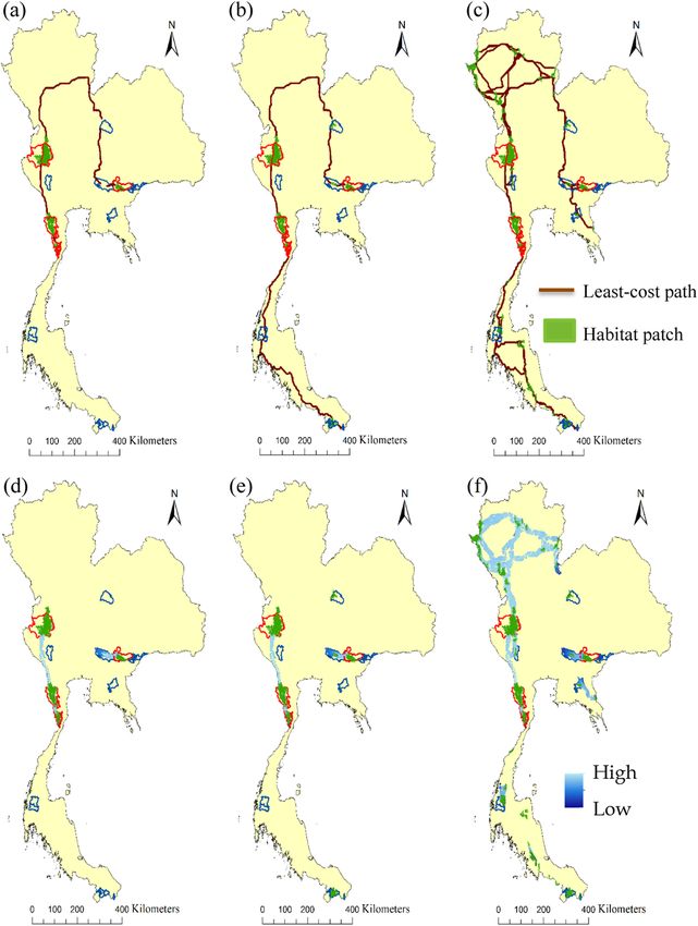
N. Suttidate et al. Global Ecology and Conservation 29 (2021) e01718
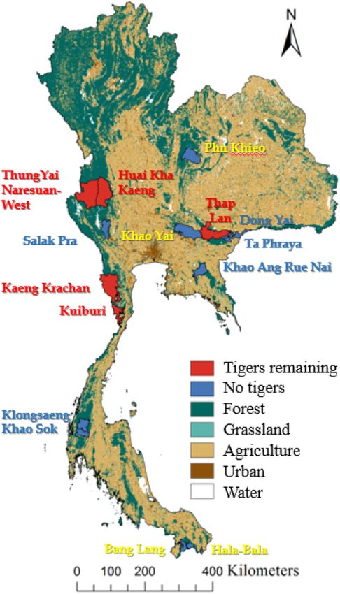
Fig. 1. Land cover across Thailand, and the 15 protected areas across Thailand where we conducted our surveys. Protected areas where tiger remain
are shaded in red. Protected areas where they no longer occur are shaded in blue and include areas where they were lost since our survey (yellow
label), and those without tiger at the time of our survey (blue label). (For interpretation of the references to colour in this figure legend, the reader is
referred to the web version of this article.)
3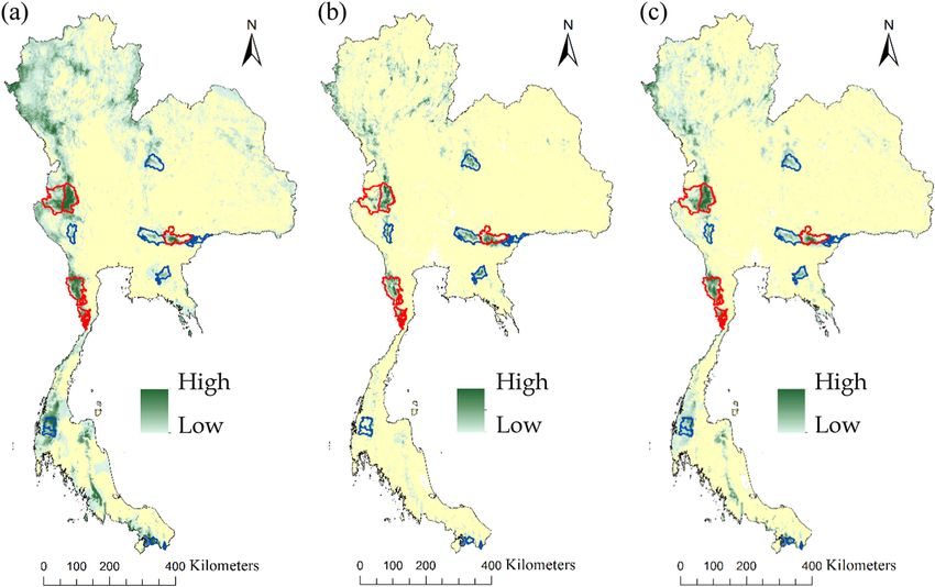
N. Suttidate et al.                                                                                      Global Ecology and Conservation 29 (2021) e01718

incomplete assessments of tiger distribution and habitat connectivity in many regions hamper conservation efforts. Thailand is one of
the regions that still needs better understanding of the patterns of tiger distributions and habitat connectivity (Duangchantrasiri et al.,
2019).
    To assess habitat connectivity for tigers, landscape elements (i.e., patches, and corridors) must allow the species to survive and
reproduce, and provide shelter, prey, absence of human disturbances which cause mortality, and connectivity to other occupied
patches for dispersal and maintenance of genetic diversity (Harihar and Pandav, 2012; Rathore et al., 2012; Joshi et al., 2013). Tigers
prefer a mosaic of forest and grassland habitats that maximize prey density, and offer cover to hunt, breed, and raise cubs. In Thailand,
such habitat is largely restricted to protected areas (Lynam, 2010; Ngoprasert et al., 2012). In terms of species interactions, tiger
distribution is primarily driven by prey availability, rather than competition with potential competitors (i.e., by leopard, cloud
leopard, and dhole) (Jenks et al., 2012; Steinmetz et al., 2013). The major prey species of tiger are wild pig, red muntjac, sambar deer,
gaur, and banteng (Ngoprasert et al., 2012; Simcharoen et al., 2018; Duangchantrasiri et al., 2019). Although tiger’s natural history is
well known, it remains unclear how prey distributions and abiotic factors together affect habitat connectivity patterns.
    Our goal was to assess habitat with tiger occurrences and potential habitat plus its connectivity for the tigers in Thailand. Our
specific objectives were to:

    (i) test our prediction that including information on primary productivity and prey results improves predictions of tiger
        occurrence;
   (ii) identify patches with tiger occurrences and potential habitat patches and dispersal corridors;
  (iii) evaluate the relative importance of habitat patches and dispersal corridors in maintaining an overall habitat connectivity
        network in order to identify priority sites for tiger and prey reintroduction.

2. Methods

   We modeled the distribution of both tigers and their prey and combined this with connectivity analyses to understand the
mechanism underlying patterns of habitat connectivity for tigers in Thailand. We employed least-cost modelling, circuit theory, and
graph theory to assess and predict habitat connectivity across Thailand. The cost-path analyses (i.e., least-cost modeling and circuit
theory) based on predicted occurrence, together with spatial data on dispersal barriers, yielded potential dispersal corridors, and graph
theory allowed us to evaluate the relative importance of habitat patches and dispersal corridors for overall connectivity.

2.1. Study area

   Thailand covers 513,000 km2 of land area between latitudes 5◦ 45 ´and 20◦ 27 ´N and longitudes 97◦ 22 ´and 105◦ 37 ´E (Fig. 1).
Elevation ranges from 0 to 2565 m. The climate is influenced by seasonal monsoons and varies by region. Only 31.6% of natural forest

Table 1
Summary of the photo camera survey data that we analyzed. Protected areas are grouped into those that had already no tigers at the time that we
conducted our surveys, those that lost tigers since our surveys, and those that had tigers when this manuscript was submitted in 2021.
                            Protected area                 Years       Trap nights   Camera            Number of photos
                                                                       (no.)         locations (no.)
                                                                                                       Tiger   Wild       Muntjac     Sambar     Gaur
                                                                                                               boar

  Areas where tigers        Huai Kha Kaeng Wildlife        1999–2011   4155          230                89     367        397         564        116
      remain                Sanctuary
                            Kaeng Krachan National         2003–2004   6893          72                  9     94         423         133        210
                            Park
                            Kuiburi National Park          2007–2011   5007          80                 25     109        58          8          77
                            Thap Lan National Park         2009–2013   2456          23                 90     2496       196         12         148
                            ThungYai Naresuan Wildlife     2007–2012   11,518        196                34     108        334         160        86
                            Sanctuary-West
  Areas that lost tigers    Bang Lang National Park        1998        803           25                 17     19         35          32         15
      since our surveys     Hala-Bala Wildlife             2004–2007   11,384        53                  3     481        399         0          0
                            Sanctuary
                            Khao Yai National Park         1999–2011   12,623        273                10     529        652         234        397
                            Phu Khieo Wildlife             1998        1486          43                  3     50         99          0          34
                            Sanctuary
  Areas without tigers in   Dong Yai Wildlife Sanctuary    2012        629           21                  0     41         10          27         8
      our surveys           Khao Ang Rue Nai Wildlife      2008–2009   6399          246                 0     41         165         254        55
                            Sanctuary
                            Khao Sok National Park         1996        246           10                  0     3          0           2          0
                            Klongsaeng Wildlife            1996        35            1                   0     3          0           0          0
                            Snactuary
                            Salak Pra Wildlife Sanctuary   2012        2688          70                  0     36         28          27         4
                            Ta Phraya National Park        1998–2012   3723          136                 0     43         94          0          23
                                                           Totals:     70,045        1479              280     4420       2890        1453       1173

                                                                             4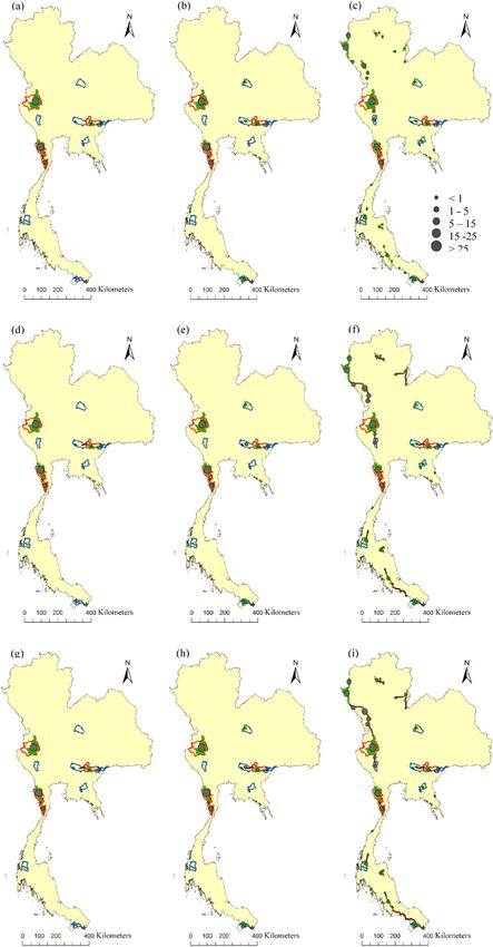
N. Suttidate et al. Global Ecology and Conservation 29 (2021) e01718
remains, mostly within protected areas at higher elevations (RFD 2017). Thailand is a global biodiversity hotspot, and home to more
than 300 mammal species, including endangered tigers (Goodrich et al., 2015).
2.2. Camera trap survey data
We collected camera trap data from 1996 to 2013 in 15 protected areas (Table 1, Fig. 1), and used the presence data of tiger and
ungulate s pecies to predict tiger occurrence and assess habitat connectivity. Cameras were located to maximize chances of capturing
animals, particularly where animal signs were found (i.e., prints and scats), on wildlife trails, stream beds, and ridges, Camera lo
cations spanned gradients in elevation (ranging from 0 to 1351 m), and habitat conditions (hill evergreen forests, mixed deciduous
forest, dry dipterocarp forest, and grassland). We attached the cameras to the base of trees about 50 cm aboveground with a minimum
distance of 0.5 km between cameras. We operated cameras 24 h per day, and cameras recorded time and date for each exposure. We
did not use baits or lures. Based on photo records, we determined for each camera location the presence or absence of tiger and their
four major ungulate prey species: Eurasian wild boar (Sus scrofa), Gaur (Bos gaurus), Red muntjac (Muntiacus muntjac), Fea’s muntjac
(M. feae), and Sambar deer (Rusa unicolor). Muntjac species were lumped for analysis. In total, we analyzed data from 70,045 trap
nights obtained from 1479 camera locations, that contained 10,216 photos of our species of interest, 280 of which were for tiger
(Table 1).
2.3. Habitat variables
We modeled tiger occurrence based on prey distributions and abiotic variables that are critical to tiger reproduction and survival.
We included (1) the probability of occurrence of the four ungulate prey species; (2) primary productivity; (3) proportion of different
habitat types; (4) mean elevation; (5) slope; (6) terrain ruggedness; (7) distance to nearest rivers and streams; (8) mean annual
precipitation; (9) distance to nearest forest edge; (10) distance to nearest human settlement and roads. We calculated values of habitat
variables at 1-km resolution (e.g., we calculated the proportion of habitat types in 1-km grid cells) and assigned them to each camera
location. This grain scale has been previously applied in the calculation of habitat variables in studies of mammalian carnivores and
ungulate prey species in Thailand (Jenks et al., 2012; Duangchantrasiri et al., 2019).
Variables associated with food availability included the probability of occurrence of four prey ungulate species, and primary
productivity. To capture primary productivity, we included cumulative annual productivity and seasonal variation in productivity,
which are two of the three Dynamic Habitat Indices (DHIs), and we used the DHIs derived from the MODIS fPAR (fraction Photo
synthetically Active Radiation) product (Hobi et al., 2017; Radeloff et al., 2019), and which we obtained from https://silvis.forest.
wisc.edu. We calculated the probability of occurrence of four prey ungulate species as a proxy for prey availability and abundance
(Ngoprasert et al., 2012; Hebblewhite et al., 2014; Simcharoen et al., 2018).
Abiotic variables included habitat types, elevation, slope, terrain ruggedness, distance to nearest rivers or streams, mean annual
precipitation, and human disturbance variables. We computed the proportion of eight habitat types: grassland, secondary forest,
bamboo forest, mixed deciduous forest, dry dipterocarp forest, hill evergreen forest, moist evergreen forest, and dry evergreen forest
according to the Thailand land cover map of 2000 provided by the Thailand Department of National Parks, Wildlife, and Plant
Conservation, which was derived from Landsat TM and ETM+ using supervised classification at a scale of 1:50,000. We calculated
mean elevation, slope (in degrees, 0–90), and terrain ruggedness from the Shuttle Radar Topography Mission (SRTM, http://srtm.csi.
cgiar.org, (Jarvis et al., 2008)). We extracted mean annual precipitation derived from averages for 1961–1990 from the WorldClim
data (https://www.worldclim.org/, (Hijmans et al., 2005)). We also calculated distance to nearest rivers or streams, forest edge, and
human settlement or road using the Thailand land cover map of 2000. We chose distance to the nearest forest edge and human set
tlement or road as a surrogate for human hunting pressure assuming that hunting intensity is inversely related to the distance that
poachers have to travel to access to wildlife habitat (Jenks et al., 2012; Lynam et al., 2012; Ngoprasert et al., 2012).
2.4. Tiger occurrence
To estimate tiger occurrence, we parameterized an ensemble model based on the camera trap data and environmental variables. An
ensemble model combines multiple Species Distribution Models (SDMs) to reach a consensus outcome for probability of species
occurrence to account for variability among SDM algorithms (Thuiller et al., 2009; Martinez-Freiria et al., 2013; Puddu and Maiorano,
2016). Initially, we included ten different species distribution modelling algorithms implemented within the BIOMOD2 package
version 3.1–64 in R (R Development Core Team 2015): three regression methods (generalized linear model, GLM; generalized additive
model, GAM; and Multiple Adaptive Regression Splines, MARS), two classification methods (flexible discriminant analysis, FDA and
classification tree analysis, CTA), and four machine-learning methods (artificial neural networks, ANN; generalized boosted model,
GBM; random forests, RF; and maximum entropy MAXENT), and a climate envelope method (surface range envelope, SRE) (Thuiller
et al., 2009; Thuiller, 2013, 2014). We applied model algorithms with default parameters. The SDM algorithms require background
data, we therefore combined true absences and generated pseudo-absences from within 70 km2 of each presence location based on
average home range size for female Indochinese tigers (Simcharoen et al., 2014). We generated 10,000 pseudo-absence location (Elith
et al., 2011).
In order to evaluate the predictive performance of the SDMs for prey species and tigers, we calculated Area Under the Curve scores
(AUC), with 10-fold cross-validation (Elith et al., 2011; Bateman et al., 2016). To provide an unbiased measure of model performance
and obtain standard deviations for evaluation metrics, we replicated data splitting 10 times (90:10 split) with the two pseudo-absence
5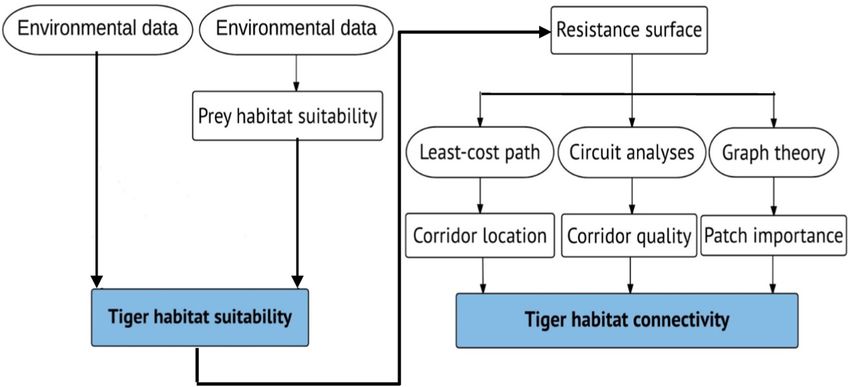
N. Suttidate et al. Global Ecology and Conservation 29 (2021) e01718
replicates (a total of 20 replicates for each model algorithm). To ensure that all replicates were comparable, we rescaled each replicate
within BIOMOD2 using a binomial GLM. We considered AUC values above 0.7 to be indicative of useful models (Thuiller et al., 2009;
Thuiller, 2014), and conducted bias-corrected null model tests. To obtain the consensus distribution for ungulate prey and tigers, we
selected the top five performing models and calculated their weighted mean distributions. In order to transform the probabilistic
consensus distribution from the ensemble model to a binary suitable/non-suitable habitat for each prey species and tigers, we
considered suitability values above the sensitivity-specificity sum maximization threshold (Phillips and Dudík, 2008; Guisan et al.,
2013).
To compare occurrence models for tigers with and without prey availability, we modeled tiger distribution with three different sets
of variables: abiotic variables alone, prey alone, or abiotic plus prey. For the tiger model with prey, we first computed species dis
tributions for the four prey ungulate species as a function of primary productivity (i.e., cumulative productivity, and seasonality in
productivity as proxies for forage availability) plus the other abiotic variables described above. To obtain the importance of the
variable for each model and each species, BIOMOD2 applies a randomization approach as one minus the correlation between the
standard predictions and predictions with randomized variables (Thuiller et al., 2009; Thuiller, 2014).
To test if prey availability significantly improved the prediction of the occurrences of the Indochinese tiger in Thailand, we
examined: (a) if the best fit model included abiotic, prey, and primary productivity variables; (b) and if model performance (i.e., AUC
values) differed significantly between the models based on abiotic model, prey model, and abiotic and prey model. We tested for
significant differences in model outputs with Wilcoxon signed-rank tests for related samples (Bateman et al., 2012).
2.5. Identifying habitat patches and dispersal corridors
We combined three methods to assess habitat connectivity for tigers: least cost modelling, circuit theory, and graph theory (Fig. 2).
We applied these methods to three sets of habitat patches. The first set included the 9 protected areas that had tigers during the time
span of our surveys (1996–2013). We included all of these protected areas, even though four have lost tigers by 2019 (Fig. 1) because
we were interested to see if the ones that lost tigers were more isolated. The second set included all 15 protected areas that we surveyed
to identify which of the ones that lacked tigers already at the time of our survey might be good candidates for reintroductions based on
their connectivity. The third set included all potential habitat patches throughout Thailand that were greater than 70 km2 based on
average home range size for female tigers in Thailand (Simcharoen et al., 2014). Similar to the second set, the third set identified
potential habitat patches that may be good candidates for reintroductions based on their connectivity.
To identify locations of dispersal corridors, we employed least-cost path modeling. We used a probabilistic occurrence map for
tigers derived from the model including prey distributions to generate least-cost path corridors for tigers. A cost surface is derived by
quantifying the resistance of different land cover classes and summing the travel cost over the route of least resistance when in
dividuals move between two patches (Adriaensen et al., 2003; Parks et al., 2013; Kaim et al., 2019). We inverted the occurrence map
for tigers with a linear function as a measure of resistance surfaces, rescaled from 1 (lowest resistance) to 100 (highest) (Ziółkowska
et al., 2012). Dispersing tigers avoid agricultural areas and human disturbance, but may travel through a mosaic of forest and grassland
with disturbed and undisturbed tracts of forest offering cover for movement (Dutta et al., 2015; Duangchantrasiri et al., 2019). We
therefore included potential dispersal barriers for tigers: agriculture area, settlement, highways, major roads, and large rivers into the
resistance surface map. To determine the position of least-cost path locations, we used the cost distance tool in ArcGIS 10.1 (ESRI
2011) with scripts written in Python 2.7 (Python Software Foundation 2013).
Fig. 2. Flowchart describing our approach to assess habitat connectivity for the Indochinese tigers in Thailand.
6
N. Suttidate et al.                                                                                 Global Ecology and Conservation 29 (2021) e01718

    To complement the least-cost path analyses, we conducted a connectivity analysis based on circuit theory. Least-cost path can
identify a corridor location, but least-cost path algorithms do not calculate optimum width for corridors, nor rank corridors in terms of
their ability to facilitate movements (Boyle et al., 2017; Dickson et al., 2019). Therefore, we applied circuit theory using Circuitscape
software (v. 4; McRae et al., 2013) to identify other potential movement routes near the least-cost path corridor and quantify how
individual tigers (i.e., electrical current) would move across the landscape within a corridor width. We buffered the least-cost paths by
10 km on each side to define dispersal corridors that are wide enough to support the tiger movement, and assessed the current between
each pairwise combination of suitable habitat patches (Brodie et al., 2015; Dutta et al., 2015).

2.6. Assessing the importance of habitat patches and dispersal corridors

     To evaluate the relative importance of individual patches and dispersal corridors for the overall connectivity network, we used the
Probability of Connectivity index (PC) based on graph theory (Pascual-Hortal and Saura, 2006; Saura and Pascual-Hortal, 2007; Saura
and Torné, 2009). PC is a graph-based metric that indicates the probability that two tigers randomly placed in the study area fall into
habitat patches that are connected. The probability of individual tigers moving between habitat patches depends on both the amount of
suitable habitat (nodes of the graph), and the distance and resistance to movement (resistance surface) across landscape matrix (links
of the graph). A graph component composed of a set of nodes corresponding to the suitable habitat patches with an area of > 70 km2.
Each pair of nodes was connected through links (least-cost paths), which indicated the potential movement paths of tigers.
     To assess the probability of connectivity, we used effective distances, that is, we replaced Euclidean distances by the cost-distance,
to calculate inter-patch-cost-dispersal probabilities (pij) as a decreasing exponential function of the effective distance between nodes
(dij) and dispersal abilities of tigers (k) (Saura and Pascual-Hortal, 2007), as follows:

         pij = e−     kd
                           ij                                                                                                                  (1)

    We set k = 0. 028, 0.012, and 0.011, which corresponds to dispersal distance of three individual tigers of 25, 58, and 64 km, and a
dispersal probability of 0.5 for each distance. These three distances correspond to three observed tiger dispersal event from Huai Kha
Kaeng Wildlife Sanctuary to Mae Wong and Klong Lan National Parks (WWF Thailand, unpublished data). These are minimum
observed distances traveled by dispersing tigers and are likely less than the actual maximal dispersal distance for tiger. Therefore, we
set the dispersal probability to 0.5 for those three distances, and conducted our analysis three times to assess how uncertainty about
actual maximum dispersal distances may have affected our results. We then computed the PC index for each landscape element (i.e.,
habitat patches, and dispersal corridors), and for each dispersal distance (Saura and Pascual-Hortal, 2007). PC index summarizes the

Fig. 3. Occurrence models for Indochinese tigers in Thailand derived from an ensemble of species distribution models showing the probability of
occurrence, (a) occurrence models based on tiger ~ abiotic variables, (b) tiger ~ prey, (c) tiger ~ prey + abiotic variables.

                                                                      7
N. Suttidate et al. Global Ecology and Conservation 29 (2021) e01718
contribution of all habitat patches to tiger movements across the whole study area, as follows
∑n ∑n
j− 1 ai aj pmax
(2)
i− 1 ij
PC =
A2L
where ai and aj are the areas of habitat patches i and j, pmax
ij is the maximum product probability of all the possible paths between habitat
patches i and j (including the direct route between the two patches), and AL is the study area.
To assess the relative importance of habitat patches and dispersal corridors to overall connectivity, we calculated d(PC)k where ‘d′
is the percentage of the importance of a given node for the connectivity according to a given index (Saura and Pascual-Hortal, 2007).
We partitioned d(PC)k into three fractions that quantify the role of each habitat patch and dispersal corridor in maintaining or
enhancing the movements of tigers with respect to habitat availability, connectivity, and stepping stone, as follows.
dPCk = dPCintrak + dPCfluxk + dPCconnectork (3)
The intra term (dPCintra k) is the contribution of habitat patch k given by the suitable habitat that it contains. The flux term
(dPCflux k) measures the degree of connection of a habitat patch k with the other habitat patches. The connector term (dPCconnector k)
corresponds to the contribution of a habitat patch and dispersal corridor k to the connectivity between other habitat patches as a
stepping-stone or connectivity facilitating dispersal between them. All three measures are reported as percentages, and larger values
indicate that a given patch or connector is more important for overall connectivity. We used Conefor 2.6 software for the graph-theory-
based analyses (Saura and Torné, 2009).
3. Results
3.1. Tiger occurrence
Our three occurrence models for the Indochinese tiger in Thailand, i.e., the abiotic model, prey model, and abiotic and prey model,
all performed well based on model accuracy for protected areas (Fig. 3). However, the incorporation of food availability significantly
improved model performance (Table 1). Of all three tiger habitat models, model accuracy was highest for abiotic and prey model (AUC
= 0.954, SD = 0.06) followed by abiotic-only model (AUC = 0.939, SD = 0.06) and prey-only model (AUC = 0.932, SD = 0.05). Model
performance was significantly different (Wilcoxon signed-rank test, P < 0.001) for all model comparisons. These results supported our
expectation that including variables that capture both primary productivity and prey distributions provides better predictions of tiger
occurrence (Table 1).
Prey occurrence was more important than abiotic factors for predicting tiger occurrences. Occurrence of tigers increased with the
probability of occurrence of wild boar (variable importance score = 0.38) and gaur (score = 0.15), the proportion of mixed deciduous
forest (score = 0.15), distance to human settlement (score = 0.17), and distance to forest edge (score = 0.12). For the abiotic model,
tiger occurrence was greater at higher proportion of mixed deciduous forest (score = 0.26), and further distance to human settlement
(score = 0.37), and forest edge (score = 0.26). The occurrence of wild boar was the best predictor of tiger occurrence in both the prey-
only and the prey plus primary productivity model.
The effect of variables on predictions of occurrence for ungulate prey varied among species. Occurrences of wild boar, gaur,
muntjac, and sambar were highly correlated with cumulative productivity, seasonality in productivity, annual precipitation, and
distance to forest edge. Occurrences of all four species increased with higher cumulative productivity. Occurrences of wild boar and
gaur were highest at a moderate level of seasonality in productivity, while seasonality in productivity had less effect on muntjac and
sambar. Occurrences of all four species were highest where annual precipitation was 1000–1500 mm, and decreased as annual pre
cipitation increased. All prey species had higher probabilities of occurrence within 1000–1500 m from forest edge.
3.2. Habitat patches
Tiger occurred in nine habitat patches during the time span of our surveys, but those patches were highly isolated (Fig. 5a). Indeed,
by 2019, four of the protected areas that had tigers at the time of our survey, and where we captured them with our cameras, no longer
Table 2
Mean model performance and ensemble measures (AUC scores) of top performing occurrence models for Tiger based on a) abiotic variables only, b)
prey variables only), and c) prey & abiotic variables, and for wild boar, gaur, muntjac, and sambar. The significance values (*** P < 0.001)are based
on Wilcoxon signed-rank test for the abiotic versus prey model, and the abiotic versus the prey & abiotic model.
Model Generalized Linear Generalized Additive Generalized Boosted Random Forest MAXENT Ensemble
Tiger: Abiotic only 0.763 ± 0.055 0.693 ± 0.068 0.784 ± 0.054 0.707 ± 0.070 0.774 ± 0.060 0.939 ± 0.06* **
Tiger: Prey only 0.735 ± 0.061 0.757 ± 0.061 0.761 ± 0.058 0.726 ± 0.071 0.772 ± 0.067 0.932 ± 0.052* **
Tiger: Prey & Abiotic 0.784 ± 0.055 0.692 ± 0.059 0.805 ± 0.043 0.734 ± 0.053 0.782 ± 0.058 0.954 ± 0.060* **
Wild boar 0.855 ± 0.017 0.858 ± 0.015 0.880 ± 0.016 0.854 ± 0.020 0.876 ± 0.016 0.962 ± 0.028
Gaur 0.790 ± 0.027 0.806 ± 0.038 0.844 ± 0.025 0.812 ± 0.030 0.825 ± 0.029 0.962 ± 0.047
Muntjac 0.896 ± 0.010 0.917 ± 0.011 0.932 ± 0.010 0.936 ± 0.011 0.930 ± 0.010 0.976 ± 0.018
Sambar 0.913 ± 0.013 0.929 ± 0.018 0.941 ± 0.009 0.904 ± 0.029 0.934 ± 0.013 0.981 ± 0.019
8N. Suttidate et al. Global Ecology and Conservation 29 (2021) e01718
harbored any (Fig. 1, unpublished data). During the time span of our surveys though, habitat patches with tiger occurrences covered a
total area of 8675 km2 ranging from 85 to 3665 km2 with a mean patch size of 528 km2, with 94.8% of the patches with tiger oc
currences inside protected areas. The largest patch was located in the Western Forest Complex (Huai Kha Kaeng, Thung Yai Naresuan,
and Mae Wong).
In terms of potential tiger habitat, i.e., areas outside of protected areas with suitable habitat, none of which had tiger occurrences
though, we identified 26 patches ranging from 74 to 1513 km2 with a mean area of 305 km2. Total area was 7929 km2, out of which
88.8% were located in protected areas. The largest patch was located in Salawin Wildlife Sanctuary (Fig. 5b).(Table 2).
3.3. Habitat connectivity and dispersal corridors
We identified seven potential corridors between the patches that with tiger occurrences at the time of our surveys (Fig. 5a). There
were only two dispersal corridors when we assumed that the probability of dispersal reaches 0.5 at 25 km in length (between Kaeng
Krachan and Kuiburi, and Banglang and Hala-Bala), and three when assuming that threshold occurs at 58 km, or ≤ 64 km length
(between Kaeng Krachan and Kuiburi, between Bang Lang and Hala-Bala, and Khao Yai and Thap Lan). Other potential corridors
among habitat patches with tiger occurrences were blocked by dispersal barriers (e.g., highways, agriculture, and urban) or were long
(> 64 km), making it difficult for tigers to disperse (Table 3). Among the potential habitat patches outside of protected areas, we
located 13 connections among suitable habitat patches of the probability of dispersal is 0.5 at 25 km, 20 connections if that occurs at
58 km, and 22 for 64 km. The circuit analyses quantified the resistance of movement for tigers within each corridor, and resistance to
movement for tigers varied considerably among the least-cost path corridors for both habitat patches with tiger occurrences and
potential habitat patches. Among the patches with tiger occurrences at the time of our surveys, the least-cost path corridor between the
Kaeng Krachan and Kuiburi habitat patches had the lowest resistance for tiger movement, meaning that there is little barrier separating
them. Conversely, the resistance for the Haui Kha Kaeng and Kaeng Krachan corridor, and the Khao Yai and Thap Lan corridor were
medium-high, thus likely inhibiting tiger dispersal (Fig. 5c, Table 3). For the resistance of movement in the dispersal corridors among
potential habitat patches, there was low resistance of movement among the least-cost path corridors in northern Thailand, which could
potentially serve as dispersal corridors connecting patches with tiger occurrences at the time of our survey to potential habitat patches
(Fig. 5d).
3.4. Importance of patches and dispersal corridors
Our graph theory analysis of the networks of the patches with tiger occurrences at the time of our survey, and of the potential
habitat patches showed that most patches were locally connected, but not regionally and much less nationally (Fig. 6). The relative
importance of habitat patches with tiger occurrences and the dispersal corridors in maintaining the overall connectivity for Indo
chinese tigers in Thailand were similar for all dispersal distances (Table 3). Among the patches with tiger occurrences at the time of our
survey, the habitat patch located in the Western Forest Complex was the most important for habitat connectivity (as quantified by the
percentage of contribution to overall connectivity; dPC = 61–63%, Table 4). This habitat patch is highly valuable because it covers a
large area of quality habitat (highest dPCintra). However, the Keng Kracha habitat patch was also well connected to other habitat
patches to which tiger populations could potentially disperse (highest dPCflux). The Kaeng Krachan habitat patch could serve as a
stepping-stone because it has a topological position that can sustain connectivity among other habitat patches (highest dPCconnector).
In terms of the relative importance of dispersal corridors between patches with tiger occurrences, the Kaeng Krachan to Kuiburi
dispersal corridor had the highest contribution to the connectivity network (dPCconnector = 9–11%) (Table 5), and the highest
dispersal probability and lowest resistance cost of movement.
Among the potential habitat patches and dispersal corridors, the Western Forest Complex habitat patch had the highest contri
bution to overall connectivity (dPC = 47–52%). The Kaeng Krachan to Kuiburi dispersal corridor was the most important linkage
Table 3
Cost dispersal probabilities (pij) and sum of cost of resistance movement (Resistance) calculated for each dispersal distance delineated dispersal
corridors between habitat patches that were occupied by Indochinese tigers at the time of our surveys. Higher values of cost dispersal probability
indicate a higher chance of movement between suitable patches. Higher values of cost of resistance movement indicate a lower chance of movement
between suitable patches.
a
Corridor Distance (km) pij 25 kmb pij 58 km pij 64 km Resistance
KK-KB 13 0.69 0.85 0.86 59.98
BL-HB 20 0.58 0.79 0.81 disconnected
KY-THP 36 0.37 0.65 0.68 223.14
HKK-KK 195 0.00 0.10 0.12 1551.59
PK-KY 258 0.00 0.05 0.06 disconnected
PK-HKK 605 0.00 0.00 0.00 disconnected
KB-BL 950 0.00 0.00 0.00 disconnected
a
KK-KB = Kaeng Krachan and Kuiburi, BL-HB = Bang Lang and Hala-Bala, KY-THP = Khao Yai and Thap Lan, Huai Kha Kaeng and Kaeng Krachan,
PK-KY = Phu Khieo and Khao Yai, Phu Khieo and Huai Kha Khaeng, and Kuiburi and Bang Lang.
b
When pij = 25 km, then the probability of dispersal at 25 km is 0.5, which means that tigers can potentially disperse further, but at a low like
lihood. When pij is 58 or 64 km, it means that the probability of dispersal drops to 0.5 at those distances, i.e,. that tigers can disperse further.
9N. Suttidate et al. Global Ecology and Conservation 29 (2021) e01718
Table 4
Contribution of each habitat patch with tiger occurrences to overall landscape connectivity as measured by the relative importance of the probability
of connectivity index dPC ( %) and its fractions for tigers’ movement assuming that the probability of dispersal drops to 0.5 at 64 km distance.
Node dPC dPCintra dPCflux dPCconnector
PK 0.77 0.61 0.16 0.00
WFC 62.85 53.15 9.69 0.00
KY 1.06 0.16 0.88 0.03
TL 3.30 2.36 0.94 0.00
KK 38.02 19.10 17.56 1.36
KB 13.57 1.71 11.86 0.00
BL 2.34 1.96 0.38 0.00
HB 0.41 0.03 0.38 0.00
Table 5
Contribution of each dispersal corridor to the maintenance of the overall landscape connectivity as measured by dPCconnector ( %) for all
tiger dispersal distances.
dPCconnector25 dPCconnector58 dPCconnector64
KK-KB 9.0 11.1 11.2
BL-HB 0.3 0.4 0.4
KY-TL 0.5 0.8 0.9
HKK-KK 0.4 6.2 7.2
PK-KY 0.0 0.0 0.1
PK-HKK 0.0 0.0 0.0
KB-BL 0.0 0.0 0.0
(dPCconnector = 6%). Several potential habitat patches and dispersal corridors located in the Western Forest Complex and northern
Thailand were important in maintaining the overall potential connectivity network, but they did not have tiger occurrences in our
surveys (Fig. 6).
4. Discussion
Our goal was to assess habitat connectivity for the endangered tiger in Thailand for areas with tiger occurrences at the time of our
surveys (1996 – 2013), and for habitat that could be potentially re-occupied by tigers. We found that incorporating primary pro
ductivity and prey distributions significantly improved predictions of occurrence for the tiger in Thailand. Tiger populations in
Thailand at the time of our survey were already confined to small, unconnected patches, and several of those areas have lost tigers since
(Fig. 1). Potential dispersal corridors between existing tiger populations were long and most had high resistance to movement. Indeed,
four of the nine protected areas where we found tigers have lost them since, and three of the four were high isolated according to our
network analyses. The connectivity networks within the Western Forest Complex and the Kaeng Krachan forest complex were the most
important for the overall functional connectivity for tigers in Thailand. Furthermore, we identified potential habitat patches that do
not contain tiger currently, but could serve as priority sites for reintroduction and dispersal corridors. However, these potential habitat
patches were highly fragmented, and regaining a connectivity network across Thailand may prove difficult.
4.1. Tiger occurrence
We found that incorporating prey distributions plus primary productivity significantly improved the predictive power of our
occurrence models, thereby providing more realistic occurrence maps for connectivity assessments. Our finding was consistent with
previous studies that tiger presence is highly dependent on prey availability, and that including prey occurrence enhances the pre
dictive performance of occurrence models (Ngoprasert et al., 2012; Hebblewhite et al., 2014; Duangchantrasiri et al., 2019). When
interpreting our maps of both tiger occurrences (Fig. 3) and occurrences of their prey (Fig. 4), it is important to note that the areas
outside of the protected areas contain no tigers at this point, and little of their prey, and represent potential habitat only. However, it is
encouraging that there are substantial areas where the environmental template is suitable for tigers and their prey, and where stronger
enforcement and reduction in poaching may permit recolonization.
Our findings also agree with those for other carnivores, where suitable habitat for connectivity networks is both a function of food
resources (e.g., prey availability, primary productivity, land cover types) and the absence of human disturbances (Jenks et al., 2012;
Ramirez-Reyes et al., 2016). For example, occurrence of grizzly bears in North America is correlated with forage-related variables (i.e.,
greenness, soil wetness, and nearest rivers), whereas cougar distributions are affected by terrain ruggedness, greenness, and avoidance
of roads (Chetkiewicz and Boyce, 2009). European brown bears occurrence is associated with forest cover, higher elevations, and
avoidance of roads and human activity in both the east-central Alps (Güthlin et al., 2011), and the Italian Alps (Peters et al., 2015). In
Borneo, abundance of sun bears (Helarctos malayanus), Sunda clouded leopards (Neofelis diardi), and banded civet (Hemigalus der
byanus) is related to elevation, logging, and road density (Brodie et al., 2015). Similarly, habitat connectivity for Jaguars depends on
10N. Suttidate et al. Global Ecology and Conservation 29 (2021) e01718
Fig. 4. Occurrence models for ungulate prey: (a) wild boar in blue, (b) gaur in purple, (c) muntjac in orange, (d) sambar deer in brown derived from
an ensemble species distribution model showing the probability of occurrence. (For interpretation of the references to colour in this figure legend,
the reader is referred to the web version of this article.)
11N. Suttidate et al. Global Ecology and Conservation 29 (2021) e01718
(caption on next page)
12N. Suttidate et al. Global Ecology and Conservation 29 (2021) e01718
Fig. 5. Connectivity across Thailand, (a) habitat patches with tiger occurrences at the time of our survey (green) and their least-cost path corridors
(brown line), (b) habitat patches in the fifteen protected areas that we surveyed and their least-cost path corridors (c) potential habitat patches and
their least-cost path corridors; and the same three sets of habitat patches with circuit theory corridors with 10 km (e-f), showing high probability of
tigers’ movements (light blue) and low probability of tigers’ movements (dark blue). (For interpretation of the references to colour in this figure
legend, the reader is referred to the web version of this article.)
land cover type, percent tree and shrub cover, elevation, and human disturbances (Rabinowitz and Zeller, 2010; Ramirez-Reyes et al.,
2016; Diniz et al., 2018). In addition to including prey availability, we integrated the cumulative annual productivity and seasonal
variation in productivity derived from the Dynamic Habitat Indices (DHIs), which have been successfully used for predictions of
species richness (Hobi et al., 2017; Radeloff et al., 2019; Suttidate et al., 2019), and the occurrence of moose in Canada (Michaud et al.,
2014), but not used to model large mammal occurrence patterns in the tropics. We found that primary productivity variables were
important factors in predicting the occurrence of both ungulate prey species, and therefore tigers in Thailand.
4.2. Connectivity assessment
We found that the remaining large, intact habitat patches for Indochinese tigers in Thailand were mostly located within protected
areas, and they were highly fragmented, with high resistance across dispersal corridors. The Western Forest Complex was the largest
contiguous area of suitable habitat, but, between it and other habitat patches, it had low dispersal probability and high resistance to
movement due to its isolation. Based on available information for Indochinese tigers in Thailand, individual tigers may not be able to
travel to the nearest patches with tiger occurrences because of urban and agricultural areas that are in-between (Simcharoen et al.,
2014; Duangchantrasiri et al., 2019). Moreover, the East-West economic corridor, a highway connecting Myanmar to Vietnam through
Thailand, which is currently being upgraded, may become increasingly a barrier that blocking tiger movement between the Western
Forest Complex and Kaeng Krachan Forest Complex. On the other hand, our results indicate that tiger populations in the Keng
Krachan-Kuiburi complex, though smaller, occur in well-connected patches and that potential dispersal corridors for tigers exist, or can
be restored.
Regaining connectivity across Thailand may prove to be difficult. Habitat connectivity remains intact only in protected areas within
the Western Forest Complex and Kaeng Krachan Forest Complex. By ranking the relative importance of each habitat patch and
dispersal corridor in maintaining the connectivity among existing tiger populations and potential suitable habitat for tigers’ dispersal,
we identified where future reintroduction could be considered if prey availability is sufficient and hunting pressure can be minimized.
We found that the habitat patch located in the Western Forest Complex was the most important refuge for tigers because it covers a
large area of suitable habitat with abundant prey (Steinmetz et al., 2008; Simcharoen et al., 2018; Duangchantrasiri et al., 2019).
However, this habitat patch is fairly isolated, which could eventually lead to inbreeding depression, as is the case for isolated tiger
populations in India and Nepal (Smith, 1993; Wikramanayake et al., 2004). The Kaeng Krachan patch has a smaller habitat area, but is
well connected to the Kuiburi habitat patch. Therefore, Keng Karchan is an important stepping-stone and dispersal corridor between
the Western Forest Complex and Kuiburi, and is the most important in maintaining the overall connectivity network in the country.
Other patches with tiger occurrences had low contribution to the overall connectivity network. A special case is the dispersal corridor
between Thap Lan and Khao Yai, which could connect relatively large suitable habitat areas. In our models, the resistance of movement
was medium-high partly because of highly 304, which runs right between the two areas. However, recently a wildlife overpass has
been constructed, and fences are being built to guide wildlife to this overpass, which may substantially reduce dispersal cost, and
provide important new connectivity.
4.3. Management implications
The remaining suitable habitat patches are located within protected areas because forested areas outside are increasingly degraded
by human activity. However, we found that these suitable habitat patches are fragmented and isolated, which is worrisome because of
the effects of habitat fragmentation on population survival, which can occur over decades (Gibson et al., 2013). It is therefore
imperative to act now to ensure long-term survival of the species. Our analyses identified several priority patches and dispersal
corridors for connectivity, where future introductions could contribute to existing tiger populations as long as prey availability is
sufficiently high, poaching can be controlled, and local communities are supportive. The north of Thailand seems particularly
promising for recolonization or reintroduction efforts. However, such efforts will require to first identify why tigers are no longer found
there, and to assess if the causes for their extirpation can be mitigated. While it is encouraging that there is ample potential habitat
according to our models, that information alone does not suffice to initiate reintroductions.
In terms of improving the connectivity of tiger populations in Thailand, we suggest several conservation strategies. First, it is
important enhance the quality of the areas where tigers remain, and where they were lost since our surveys, by decreasing land use
pressure in the potential habitat patches outside of protected areas, and controlling poaching. Second, we recommend protecting po
tential habitat patches and dispersal corridors identified by our study. Third, it is necessary to maintain high-value habitat patches and
dispersal corridors to ensure persistence of a connectivity network. Fourth, it will be valuable to restore degraded habitat through
strategic land-use planning so that prey species population can increase. These four steps, in addition to improving the connectivity of
tiger population in Thailand would also improve habitat quality and connectivity for their prey species, thereby providing both addi
tional conservation benefits (gaur and sambar deer are both ranked as ‘vulnerable’ by IUCN), and higher prey availability for tigers.
13N. Suttidate et al. Global Ecology and Conservation 29 (2021) e01718
14 (caption on next page)N. Suttidate et al. Global Ecology and Conservation 29 (2021) e01718
Fig. 6. The relative importance of habitat patches and dispersal corridors for the Indochinese tigers in Thailand. The importance of each habitat
patch is shown in term of its contribution to maintain the overall landscape connectivity as measured by the probability of connectivity index for
occupied at the time of our surveys, all fifteen protected areas, and potential habitat patches: (a), (b), and (c) probability of dispersal is 0.5 at 25 km
distance, (d), (e), and (f) at 58 km, (g), (h), and (i) at 64 km.
In summary, the goal for tiger conservation is to create large and well-connected populations that can persist long-term. We found
that the habitat connectivity network for the Indochinese tigers in Thailand consists of highly isolated patches. However, we highlight
priority areas for conserving existing tiger populations, and potential candidate sites for future reintroductions and potential dispersal
corridors. It is crucial to protect both remaining and potential habitat patches and corridors. Enhancing the quality of the area where
tigers remain, and reintroducing tiger populations and their prey in other areas could substantially increase the overall connectivity
among the Indochinese tiger populations in Thailand. Our connectivity analyses also highlight the importance of incorporating prey
distributions plus primary productivity interactions to quantify occurrence, and demonstrate how combining least-cost modeling,
circuit analysis, and graph theory approaches with species’ dispersal ability can improve assessments of habitat quality and con
nectivity. This information is important for understanding patterns of habitat connectivity and for developing management strategies
to ensure long-term survival of tigers and other carnivores in Thailand.
Declaration of Competing Interest
The authors declare that they have no known competing financial interests or personal relationships that could have appeared to
influence the work reported in this paper.
Acknowledgments
We are thankful for funding from the NASA Biodiversity Program, The NASA Program for the Science of Aqua and Terra, and the
Royal Thai Government. We are grateful to the following institutions for allowing us to used field survey data: the Wildlife Conser
vation Society Thailand, Keidanren Nature Conservation Fund, The Rhino and Tiger Conservation Fund (U.S. Fish and Wildlife Ser
vice), Sheila and Francois Brutsch, WWF Germany, WWF France, WWF US, Smithsonian Institution, Kasetsart University, and King
Mongkut’s University of Technology Thonburi. This research was carried out in collaboration with the Department of National Parks,
Wildlife, and Plant Conservation for allowing us to access the Thailand land cover map. We thank M. Dubinin for the Dynamic Habitat
Index data. We thank to A. Pidgeon, B. Zuckerberg, M. Ozdogan, and I. Baird, and two anonymous reviewers for their helpful com
ments on earlier drafts of the manuscript.
Appendix A. Supporting information
Supplementary data associated with this article can be found in the online version at doi:10.1016/j.gecco.2021.e01718.
References
Adriaensen, F., Chardon, J.P., De Blust, G., Swinnen, E., Villalba, S., Gulinck, H., Matthysen, E., 2003. The application of ‘least-cost’ modelling as a functional
landscape model. Landsc. Urban Plan. 64, 233–247.
Albert, C.H., Rayfield, B., Dumitru, M., Gonzalez, A., 2017. Applying network theory to prioritize multispecies habitat networks that are robust to climate and land-use
change. Conserv. Biol. 31, 1383–1396.
Araújo, M.B., Luoto, M., 2007. The importance of biotic interactions for modelling species distributions under climate change. Glob. Ecol. Biogeogr. 16, 743–753.
Bateman, B., VanDerWal, J., Williams, S., Johnson, C., 2012. Biotic interactions influence the projected distribution of a specialist mammal under climate change.
Divers. Distrib. 18, 861–872.
Bateman, B.L., Pidgeon, A.M., Radeloff, V.C., VanDerWal, J., Thogmartin, W.E., Vavrus, S.J., Heglund, P.J., 2016. The pace of past climate change vs. potential bird
distributions and land use in the United States. Glob. Change Biol. 22, 1130–1144.
Beier, P., Spencer, W., Baldwin, R.F., McRae, B.H., 2011. Toward best practices for developing regional connectivity maps. Conserv. Biol. 25, 879–892.
Boyle, S.P., Litzgus, J.D., Lesbarreres, D., 2017. Comparison of road surveys and circuit theory to predict hotspot locations for implementing road-effect mitigation.
Biodivers. Conserv. 26, 3445–3463.
Breckheimer, I., Haddad, N.M., Morris, W.F., Trainor, A.M., Fields, W.R., Jobe, R.T., Hudgens, B.R., Moody, A., Walters, J.R., 2014. Defining and evaluating the
umbrella species concept for conserving and restoring landscape connectivity. Conserv. Biol. 28, 1584–1593.
Brodie, J.F., Giordano, A.J., Dickson, B., Hebblewhite, M., Bernard, H., Mohd-Azlan, J., Anderson, J., Ambu, L., 2015. Evaluating multispecies landscape connectivity
in a threatened tropical mammal community. Conserv. Biol. 29, 122–132.
Brodie, J.F., Mohd-Azlan, J., Schnell, J.K., 2016. How individual links affect network stability in a large-scale, heterogeneous metacommunity. Ecology 97,
1658–1667.
Carvajal, M.A., Alaniz, A.J., Smith-Ramírez, C., Sieving, K.E., Syphard, A., 2018. Assessing habitat loss and fragmentation and their effects on population viability of
forest specialist birds: linking biogeographical and population approaches. Divers. Distrib. 24, 820–830.
Chetkiewicz, C.-L.B., Boyce, M.S., 2009. Use of resource selection functions to identify conservation corridors. J. Appl. Ecol. 46, 1036–1047.
Dickson, B.G., Albano, C.M., Anantharaman, R., Beier, P., Fargione, J., Graves, T.A., Gray, M.E., Hall, K.R., Lawler, J.J., Leonard, P.B., Littlefield, C.E., McClure, M.L.,
Novembre, J., Schloss, C.A., Schumaker, N.H., Shah, V.B., Theobald, D.M., 2019. Circuit-theory applications to connectivity science and conservation. Conserv.
Biol. 33, 239–249.
Diniz, M.F., Machado, R.B., Bispo, A.A., Brito, D., 2018. Identifying key sites for connecting jaguar populations in the Brazilian Atlantic Forest. Anim. Conserv. 21,
201–210.
15You can also read