Geometric Optimization of Nonequilibrium Adiabatic Thermal Machines and Implementation in a Qubit System
←
→
Page content transcription
If your browser does not render page correctly, please read the page content below
PRX QUANTUM 3, 010326 (2022)

                Geometric Optimization of Nonequilibrium Adiabatic Thermal Machines and
                                    Implementation in a Qubit System
                Pablo Terrén Alonso ,1,*,† Paolo Abiuso ,2,3,† Martí Perarnau-Llobet ,3 and Liliana Arrachea                    1
           1
               International Center for Advanced Studies, Escuela de Ciencia y Tecnología and ICIFI, Universidad Nacional de
                                 San Martín, Avenida 25 de Mayo y Francia, Buenos Aires 1650, Argentina
                  2
                    ICFO—Institut de Ciéncies Fotóniques, The Barcelona Institute of Science and Technology, Castelldefels,
                                                          Barcelona 08860, Spain
                           3
                             Département de Physique Appliquée, Université de Genéve, Genéve 1211, Switzerland

                 (Received 14 October 2021; revised 20 December 2021; accepted 25 January 2022; published 16 February 2022)

                     We adopt a geometric approach to describe the performance of adiabatic quantum machines, operating
                  under slow time-dependent driving and in contact with two reservoirs with a temperature bias during all the
                  cycle. We show that the problem of optimizing the power generation of a heat engine and the efficiency
                  of both the heat engine and refrigerator operational modes is reduced to an isoperimetric problem with
                  nontrivial underlying metrics and curvature. This corresponds to the maximization of the ratio between
                  the area enclosed by a closed curve and its corresponding length. We illustrate this procedure in a qubit
                  coupled to two reservoirs operating as a thermal machine by means of an adiabatic protocol.

                  DOI: 10.1103/PRXQuantum.3.010326

                        I. INTRODUCTION                                  refrigerators [17–19] are seminal examples of this type of
                                                                         operation.
   The development and implementation of thermody-
                                                                            When the WS is connected at the same time to two
namic processes in few-level quantum systems is currently
                                                                         or more thermal reservoirs, it is permanently thread by a
a very active area of research. Thermodynamic cycles con-
                                                                         heat flux. Hence, the very operation as a machine relies
ceived for macroscopic working substances (WSs), such
                                                                         on the mechanism of heat-work conversion in order to
as the Otto or Carnot cycle, are now realized in single
                                                                         overcome this effect as well as the dissipation generated
atoms [1–6] and large theoretical efforts are devoted to
                                                                         by the driving sources. The optimal machine is the one
its characterization and optimization at the microscopic
                                                                         leading to the optimal balance between these two pro-
scale [7–15]. In these standard thermodynamic cycles, the
                                                                         cesses. In quantum systems, the operation under a small
WS operates in four steps, of which two are in contact
                                                                         temperature bias and “adiabatic driving” through parame-
with reservoirs at different temperatures connected one at
                                                                         ters, which slowly vary in time, is of paramount relevance,
a time, while the other two steps consist in an evolution
                                                                         since this is an appealing scenario to control the nonequi-
decoupled from the reservoirs. It is however typically hard
                                                                         librium mechanisms. In this regime, the period of the cycle
to fully isolate a quantum WS from the environment, which
                                                                         is larger than any characteristic time of the quantum sys-
is required to emulate ideal classical cycles. This motivates
                                                                         tem, including the relaxation time between system and
the study of nonequilibrium systems, where the driven WS
                                                                         reservoirs [20–26].
is permanently in contact with two or more reservoirs.
                                                                            Recently, it was proposed that the dissipation and
Unlike standard thermodynamic cycles, these microscopic
                                                                         the heat-work conversion mechanisms are, respectively,
machines operate away from equilibrium during all the
                                                                         described by different components of the thermal geomet-
cycle. Thermoelectric devices [16] as well as autonomous
                                                                         ric tensor. Furthermore, the heat-work conversion compo-
                                                                         nent can be expressed in terms of a Berry-type phase [15],
                                                                         which has an associated Berry-type curvature [27], and
  *
      pterren@unsam.edu.ar                                               similar ideas were followed in Refs. [28,29]. Hence, a
  †
      These two authors contributed equally.                             length and an area in the parameter space can be defined.
                                                                         Besides, it is well known that dissipation and entropy
Published by the American Physical Society under the terms of            production admit a geometric description in terms of the
the Creative Commons Attribution 4.0 International license. Fur-
                                                                         concept of thermodynamic length [30–39]. This geometric
ther distribution of this work must maintain attribution to the
author(s) and the published article’s title, journal citation, and       approach has proven useful to optimize finite-time ther-
DOI.                                                                     modynamic processes (examples can be found in Refs. [9,

2691-3399/22/3(1)/010326(17)                                      010326-1               Published by the American Physical Society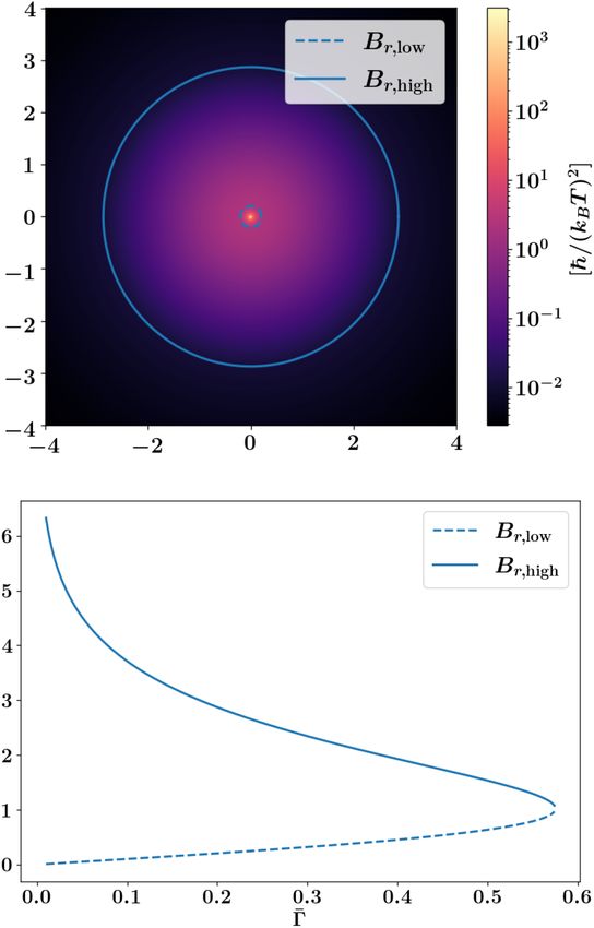
TERRÉN ALONSO, ABIUSO, PERARNAU-LLOBET, and ARRACHEA                                         PRX QUANTUM 3, 010326 (2022)

40–42] for classical and Refs. [12,43,44] for quantum                The paper is structured as follows. In Sec. II, we intro-
systems), including the finite-time Carnot cycle [11,12]           duce the setup and define the relevant thermodynamic
and slowly driven engines [45–49]. As mentioned before,           quantities to characterize the cycle. In Sec. III, we describe
these cycles are characterized by the WS being coupled to         the underlying geometry of the system. In Sec. IV we
a single reservoir or completely decoupled from reservoirs.       describe the heat engine and refrigeration modes of the
   The aim of the present work is to optimize the per-            machine, and perform the optimization with respect to the
formance of thermal machines with cycles in permanent             driving time. In Sec. V, we develop the full optimization
contact with two or more reservoirs at different tempera-          of the machine. We then compute in detail all the relevant
tures by a geometrical approach. To this end, we combine          quantities in a model of one of the most paradigmatic and
the geometrical description of the two competing mech-            simplest quantum engines, namely a driven qubit system
anisms of the nonequilibrium thermal machine (namely              (see Refs. [12,15,62]).
heat-work conversion and dissipation) in order to find
optimal protocols for maximizing power generation of                II. THE SETUP AND ITS THERMODYNAMICS
the heat-engine operation and the efficiency of the heat
                                                                     We focus on the usual configuration where the WS oper-
engine and refrigerator operational modes. We show that
                                                                  ates in contact with two reservoirs at different temperatures
the problem of finding such optimal protocols reduces to
                                                                  Th (hot) and Tc (cold), with Th = T + T and Tc ≡ T.
an isoperimetric problem [50] (also studied as the Cheeger
                                                                  A particular example, which is studied in detail in forth-
problem [51,52]), that is the task of finding the shape
                                                                  coming sections, is sketched in Fig. 1. The full system is
that maximizes the ratio between area and length. This is
                                                                  described by the Hamiltonian
one of the oldest geometric problems in history, and was
solved already by the ancient Greeks in the standard two-
                                                                            H(t) =        Hα + Hcont,α + HWS (t).          (1)
dimensional Euclidean plane [53]. Nevertheless, when the
                                                                                     α=c,h
underlying area density or length metrics are nontrivial
[54–57], no general solution is known.                            The Hamiltonian for the WS depends on time through a
   We illustrate these ideas in a prominent quantum sys-          set of control parameters Bj (t), j = 1, N , which we enclose
tem playing the role of the WS: a qubit driven by two                             = [B1 (t), . . . , BN (t)]. Hence, HWS (t) =
                                                                  in a vector B(t)
parameters slowly changing in time and asymmetrically
                                                                  HWS [B(t)]. We are interested in cycles, so that we con-
coupled to two thermal reservoirs at different tempera-            sider time-dependent protocols satisfying B    (t + τ ) = B(t),

ture (see Fig. 1). We show analytically that the limiting         being τ the period of the cycle. The reservoirs are repre-
value for the area in the parameter space is given by the         sented by the Hamiltonian
celebrated Landauer bound [58,59], which has been the
motivation of many studies including several experiments                                       †
                                                                                Hα =      εkα bkα bkα , α = c, h,              (2)
(e.g., Refs. [60,61]). We also find that, operating as a heat
                                                                                        k
engine, the qubit thermal machine offers a very good ratio
between generated power and efficiency in a wide range of                          †
                                                                  with bkα and bkα being the annihilation and creation opera-
parameters.                                                       tors of a bosonic excitation. The coupling is represented by

                                                                                                             †
                                                                               Hcont,α =      Vkα π̂α bkα + bkα ,          (3)
                                                                                              k

                                                                  where π̂α is a matrix with the dimension of the Hilbert
                                                                  space of the WS.
                                                                     The crucial concepts that characterize the operation of
                                                                  the thermal machine are the work performed and the net
                                                                  heat exchanged between the two reservoirs during the
                                                                  cycle. The operation of the driven quantum system as a
                                                                  thermal machine in the presence of a temperature bias
                                                                  relies on the mechanism of heat-work conversion. In the
                                                                  present case, we make two main assumptions:

FIG. 1. Schematic configuration of the setup. A working sub-          (i) slow driving [26], characterized by a small rate of
stance WS is in contact with two reservoirs at different temper-          change of the driving parameters with time, dt B
atures, Tc and Th . The state ρ̂ of the system changes at slow                             as well as
                                                                         [short for (d/dt)B],
but finite speed along a closed path defined by the Hamiltonian       (ii) a small temperature bias T between the two reser-

H[B(t)]  in a quasistatic process.                                       voirs.

                                                            010326-2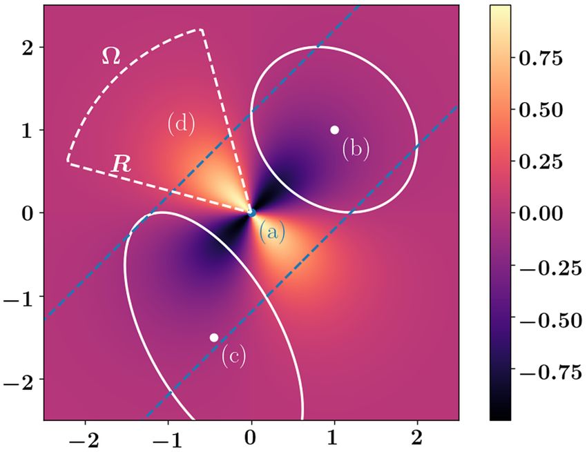
GEOMETRIC OPTIMIZATION OF NONEQUILIBRIUM. . .                                                            PRX QUANTUM 3, 010326 (2022)

This enables us to work in the linear-response regime with                        that the fundamental component for the thermal machine to
                                                                                                                                  τ
respect to dt B and T.                                                          operate is the heat-work conversion term 0 dt  · dt B.  In
    A natural theoretical framework in this context is the                        fact, without this component, the only surviving processes
adiabatic linear response theory proposed in Ref. [63] in                         are the dissipation of the energy supplied by the driving
the geometric perspective of Ref. [15]. This formalism                            forces and the trivial conduction of heat as a response to
applies to the regime where the period of the cycle is                            the thermal bias.
much larger than the longest time scale characterizing the                           The different terms in Eqs. (6) and (7) can be reinter-
WS coupled to the reservoirs. In most of the cases, such                          preted geometrically, as explained in the following Sec. III.
a time scale is determined by the relaxation time τrel of                         This allows for the optimization of the thermodynamic
the WS with the reservoirs. More precisely, the dynami-                           protocols in terms of clear geometrical quantities.
cal perturbation to the steady state ρ̂B (corresponding to                           It is important to notice that the second terms of Eqs. (6)
no driving, i.e., “frozen” value of B), can be estimated to                       and (7) have a defined sign. In our convention, is pos-
δ ρ̂ ∼ τrel (∂B ρ̂B )dt B (cf. Refs. [15,26,63] or Appendix A 1).                 itive definite since it is directly related to the entropy
Hence, this approach is useful when τ  τrel . We also con-                       production rate [15], which means that it is detrimental
sider small temperature bias, such that T/T  1. This                            for the work output. Similarly, κ can be seen to be pos-
description leads to a linear relation between the relevant                       itive, as a consequence of the fact that this component
energy fluxes operating the cycle and the components of                            of the transferred heat describes the flux from the hottest
the vector dt X = (dt B,    T/T). The relevant quantities are                   to the coldest reservoir. These are direct consequences of
the net output work and transferred heat between the hot                          the second law of thermodynamics. Instead, the line inte-
                                                                                           τ
and cold reservoirs. They are, respectively, defined as the                        gral 0 dt  · dt B may have any sign, depending on the
average over one period of the power developed by the                             driving protocol and it is enough to time reverse the func-
driving sources, and the energy flux into the α reservoir,                                 to flip the sign. As mentioned before, this term
                                                                                  tion B(t)
                                                                                describes the heat-work conversion process and its sign
                                 τ
                                                 ∂ HWS                            defines the type of operation of the machine. In fact, when
                W=−                  dt
                                                        · dt B,             (4)
                             0                     ∂ B                           it is negative, the contribution of the first term of Eq. (7)
                                        τ                                        may overcome the heat flowing into the coldest reservoir
                         i
               Qα = −                        dt[Hα , H],                  (5)   and enable the operation of the machine as a refrigerator.
                                    0                                            This has an associated cost, described by the first term of
                                                                                  Eq. (6), which must be developed by the driving sources.
where O = Tr [ρO], ρ is the global state of system and                                                                τ
                                                                                  In the opposite situation where 0 dt  · dt B ≥ 0, the first
baths (which in general will be correlated due to the
                                                                                  term of Eq. (6) may overcome the second one, enabling the
contacts). The corresponding expectations values are eval-
                                                                                  mechanism of work output. This has an associated extra
uated in linear response with respect to dt X. In such a
                                                                                  heat transfer from the hot to the cold reservoirs, which
regime Qc = −Qh ≡ Q [64]. The result is
                                                                                  is accounted for the first term of Eq. (7). This operation
                                τ                                               corresponds to a heat engine.
          T τ
       W=
                   dt · dt B −      dtdt B ·
                                                                  · dt B,   (6)
           T 0                   0
           τ                                                                            III. GEOMETRY OF THE PROBLEM
                             T τ
       Q=     dt  · dt B +         dtκ.                                   (7)
           0                  T 0                                                    We now elaborate on the geometrical interpretation of
                                                                                  the quantities presented in the previous section.
These expressions can be derived in the adiabatic linear-                            First, we factorize the total duration τ in the expres-
response regime as from Ref. [15] and we defer the reader                         sions, Eqs. (6) and (7), such to decouple the time rescaling
to that paper for further details. For the moment it is                           from the geometrical contribution to the different quanti-
enough to stress that { ,  , κ} are all local functions of                       ties. Indeed by considering an adimensional time unit θ
  while they also depend on the coupling parameters, the
B,                                                                                such that
density of states of the thermal baths and T.
   In Eq. (6), the first term represents the mechanism of                                           = B(θτ
                                                                                                        ),
                                                                                                  B(t)                   θ ∈ [0, 1],        (8)
heat-work conversion and the second one corresponds to
finite-time dissipation developed by the time-dependent
controls.                                                                         we can define, identifying from now on the adimensional
   Moreover, in Eq. (7), the transferred heat Q also contains                     time derivative B˙ ≡ ∂ B/∂θ

                                                                                                               = τ dt B,
two terms associated with two different physical processes.
The first one describes the heat exchange between the                                                             1
reservoirs related to the driving while the second one is the                                          A=                    ˙
                                                                                                                      dθ  · B,             (9)
heat transport as a response to the temperature bias. Notice                                                  0

                                                                            010326-3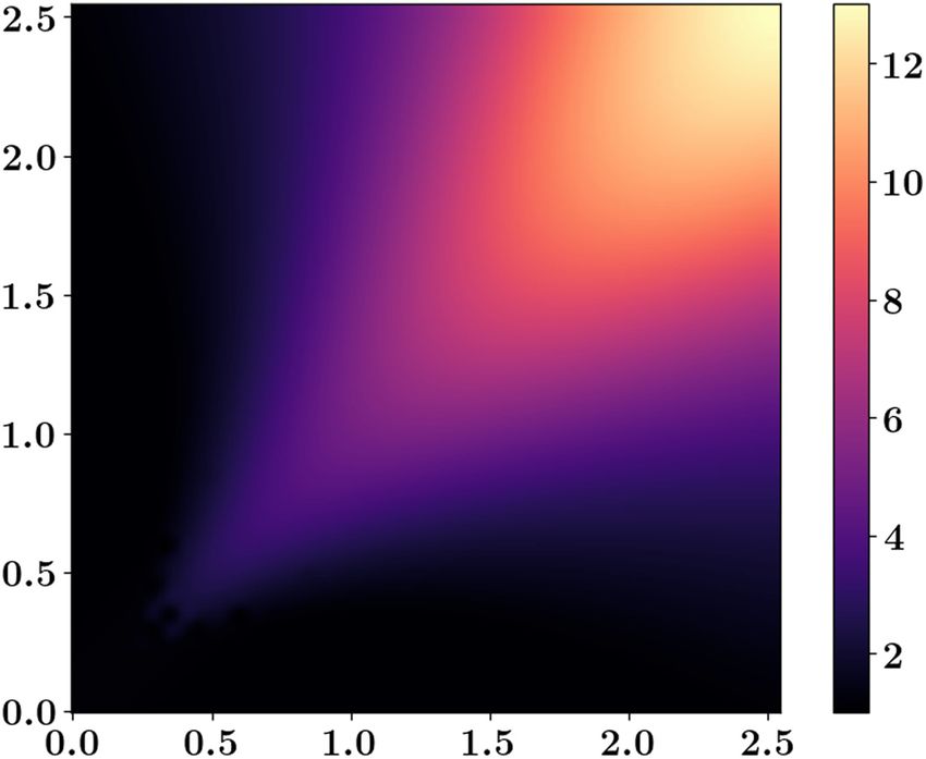
TERRÉN ALONSO, ABIUSO, PERARNAU-LLOBET, and ARRACHEA                                           PRX QUANTUM 3, 010326 (2022)
                                    1
                                         dθ B˙ ·     ˙          therefore interested in its minimum value, which can be
                     L =
                      2
                                                    · B,   (10)   obtained through a Cauchy-Schwarz inequality
                                 0
                                    1                                                               2
                                                                               1                                                        2
                     κ =
                                 0
                                         dθκ.              (11)   L ≥
                                                                   2
                                                                                   dθ B˙ ·   · B˙       =           dB ·     · dB       ≡ L2 .
                                                                           0                                    ∂

   Accordingly, Eqs. (6) and (7) can be expressed as                                                                                         (15)
follows:                                                          The lower bound L is fully geometric (it depends solely
                        T     L2                                 on ∂ ) and it is always achievable by choosing the time
                  W=       A− ,                 (12)
                        T       τ                                 parametrization θ such that B˙ · · B˙ is constant. L is a
                           T                                     natural extension of the standard thermodynamic length
                  Q=A+         τ κ.           (13)
                            T                                     [9,30–37,42,44,68] to nonequilibrium setups where the
                                                                  WS is simultaneously interacting with several baths.
   The names A and L2 are related the geometrical meaning            Finally, it is apparent that κ Eq. (11) represents the
of the quantities above, as we discuss below. The repre-          simple average of a scalar number (the heat conductance)
sentation of Eq. (9) highlights the fact that A corresponds       along the trajectory. In general, it clearly also depends on
to a Berry-type phase in the parameter space as discussed         reparametrizations of the adimensional time θ (θ ), as the
in Ref. [15]. Notice, that, in order to have a nonvanish-         average can be arbitrarily close to the maximum value κmax
ing value of A, at least two time-dependent parameters            of the trajectory, in case θ is such to spend almost all the
are necessary. This is basically the same argument widely         time close to κmax . Similarly κ can be arbitrarily close to
discussed in the literature of adiabatic charge pumping           the minimum value along the trajectory κmin .
[21,23,65,66]. In addition, it is necessary to break some
symmetries in the system to have a finite value of this                 IV. PERFORMANCE OF THE MACHINE AND
closed integral [15], as discussed below.                                       TIME OPTIMIZATION

   Given that B(θ)  represents a closed trajectory in space,
we can use Stokes’ theorem—in a three-dimensional                    In this section we discuss the different operation modes
space or its corresponding generalization in higher dimen-        of the thermal machine, and introduce the relevant figures
sions—to re-express the line integral defining A                   of merit for its characterization.
                                                                                            A. Heat engine
           A=
                       · dB = (∇   B ∧  ) · d  ,     (14)
                 ∂                                                   The system described in the previous sections can be
                                                                  used to extract work from two reservoirs with a tempera-
where      is a surface in the B space, with boundary ∂          ture bias. This is the engine operating mode of the system.
coinciding with the control trajectory. In the case of hav-       We write the power of the heat engine and its efficiency as
ing four or more parameters, Eq. (14) should be replaced
                                                                                         W   T A[1 − (τD /τ )]
by the generalized Stokes’ theorem applied to differential                             P=   =                    ,                            (16)
forms in the appropriate dimension [67]. In this represen-                               τ    T         τ
tation, A is the flux of the vector ∇ B ∧  through the area                             W      1 − (τD /τ )
                                                                                      η=   = ηC              ,                               (17)
enclosed by the control trajectory, and can be also inter-                               Q      1 + (τ/τk )
preted as the integral over this area weighted by the Berry
curvature [27]. We can therefore think of A as the area of        where we substitute Eqs. (6) and (7) and we define the
the surface defined by the control trajectory (with local         dissipation and heat-leak time scales
weight depending on the Berry curvature). Note that this
                                                                                              T L2                   T A
geometrical translation clarifies as well that A depends                               τD =         ,          τκ =          .                (18)
only on the geometry of the trajectory B(θ   ): that is, not                                 T A                   T κ
only is A independent of τ , but it is also invariant under       In the previous expressions ηC = T/T is the Carnot effi-
any reparametrization θ (θ ), which might change the local        ciency. Given the expressions above, we can optimize the
speed and time spent on different points of the trajectory.        duration of the cycles in order to maximize the power or
   Concerning L2 , it can be interpreted as a length squared      the efficiency, obtaining correspondingly
                            ), as it is clear from Eq. (10)
of the control trajectory B(θ

that it represents the integral of a quadratic form that                    τP = 2τD , τη = τD + τD (τD + τκ ).       (19)
defines a metric in the B space. At the same time, given the
presence of two time derivatives, L2 can depend in general        We see that the duration for maximum efficiency is always
on reparametrizations θ (θ ). However, L2 represents losses       larger than the duration for maximum power. The cor-
due to dissipation in the driving—see Eq. (6)—and we are          responding maximum power and efficiency at maximum

                                                            010326-4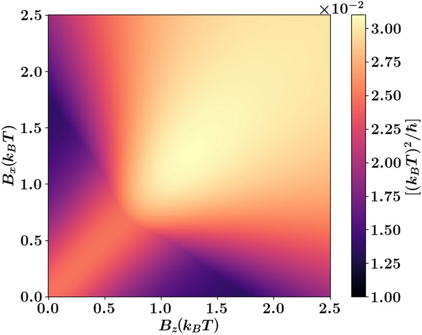
GEOMETRIC OPTIMIZATION OF NONEQUILIBRIUM. . .                                                     PRX QUANTUM 3, 010326 (2022)

        1.2                                                   1.2          the cooling power P and the coefficient of performance
        1.0                                                   1.0          (COP) η
        0.8                                                   0.8
                                                                                               −Q      1 − (τ/|τk |)
                                                                                           P =     =A                 ,             (23)
        0.6                                                   0.6                               τ            τ
        0.4                                                   0.4                              Q       1 − (τ/|τk |)
                                                                                           η =    = ηC                ,             (24)
        0.2                                                   0.2                              W       1 + (|τD |/τ )
        0.0
              1           2       3      4         5      6
                                                              0.0
                                                                           where ηC = T/T is the Carnot COP. The difference with
                                                                           the engine operating mode is that in this case both Q and
                                                                           W are negative (heat is transferred against the thermal bias
FIG. 2. Engine mode: power and efficiency versus cycle dura-                 and work is performed on the system). We have therefore
tion. The optimal operating region is the gray interval between            A < 0, which implies τκ < 0 and τD < 0 are formally neg-
the two dashed lines: indeed for any point outside the region,             ative as well (which is the reason of the absolute values
there is a point inside with both larger efficiency and larger               in the equations). By direct inspection of Eq. (23) we see
power. In the limit of big heat leaks κ, the corresponding heat-         that the maximum power of such a mode is unbounded, as
leak time scale τκ , Eq. (18), is small, and the difference between         in the limit τ → 0 the power tends to infinity. The slow-
τP and τη , Eq. (19), shrinks. That is, when the heat leak is the
                                                                           driving approximation τrel /τ  1 prevents us from ana-
dominant loss, power and efficiency maximization tend to coin-
cide, as one could expect [this can be verified by direct inspection        lyzing the limit of arbitrary small τ and a reliable analysis
of Eqs. (16) and (17)]; the corresponding maximum efficiency is              of the cooling power requires a description beyond linear
also small in this limit. In the opposite limit of no leaks κ → 0,       response [69,70]. Thus, we focus only on maximizing the
τκ tends to infinite, and we recover the standard scenario in which         efficiency of this operation, for which we get
power is maximized for a finite time, while the efficiency is max-

imum for τ → ∞, where it tends to the Carnot efficiency, as the                            τη = τη =    τD (τD + τκ ) − |τD |,        (25)
dominant loss is due to finite-time dissipation. For finite values of
κ, the scenario is intermediate. In the plot τD = 1 and τκ = 2.5.                             T          2
                                                                                       ηmax =        1− √     ,                     (26)
                                                                                                T        x+1
power are                                                                                       T √
                                                                                      Pηmax   =    κ x,                           (27)
                                                                                                T
                  1 (T)2 A2                     ηC x − 1
       Pmax =                ,        ηPmax =             ,         (20)   with x defined as in Eq. (22).
                  4 T 2 L2                        2 x+1
                                                                                    V. FULL OPTIMIZATION AND THE
while the maximum efficiency and power at maximum
                                                                                        ISOPERIMETRIC PROBLEM
efficiency
                                                                              In the previous section we showed how to choose
                                        2                                  the optimal duration for cycles of two kinds of ther-
                  ηmax    = ηC 1 − √          ,                            mal machines, and we derived formal expressions for the
                                       x+1
                                       √                                   resulting powers and efficiencies. The resulting figures of
                            (T)2     ( x − 1)2                            merit still depend on the particular trajectory chosen for the
                  Pηmax   =       κ     √     ,                   (21)
                              T2            x                              cycle. Finding the fully optimal solution is nontrivial, but
                                                                           we show in the following how the geometrical picture of
with                                                                       the thermodynamics introduced in Secs. III and IV, helps
                                                                           in finding the most advantageous control trajectories to be
                                       A2                                  exerted on the machine.
                              x =1+          .                      (22)      An interesting question in the present problem is
                                      L2 κ
                                                                           whether we can find a protocol that maximizes the output
See Fig. 2 for a summary and visual explanation of these                   power of the system. We have shown in Sec. III that, given
                                                                                                ) defined over ∂ in the parameter
                                                                           a parametrization B(θτ
results.
                                                                           space, we can compute the duration τ that upper bounds
                                                                           the power for that protocol. The result is expressed in
                              B. Refrigerator                              Eq. (20). Besides, we know from the definition in Eq. (14)
   In the heat pump or refrigerating mode, external work                   that the value of A2 does not depend on reparametriza-
is supplied to the system to extract heat from the cold                    tions θ , while the value of L2 can be lower bounded by
bath and transfer it to the hot one. Therefore, we define                   L2 according to Eq. (15). With all these considerations,

                                                                     010326-5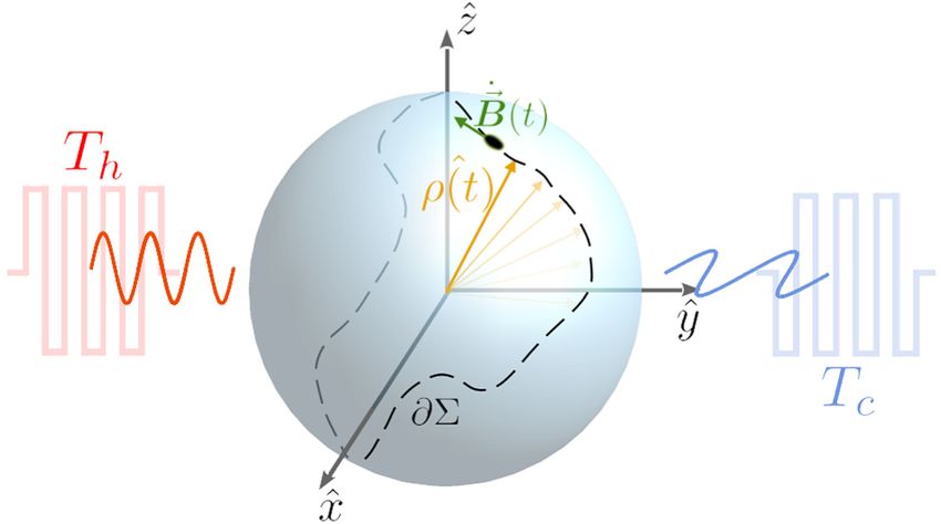
TERRÉN ALONSO, ABIUSO, PERARNAU-LLOBET, and ARRACHEA                                             PRX QUANTUM 3, 010326 (2022)

we find that the maximum power developed by a protocol                  As already highlighted in Sec. II, a key ingredient
moving along a curve ∂ is expressed by                              to have the heat-work mechanism in the linear-response
                                                                    regime, is some protocol leading to A = 0. We recall
                                     1 (T)2 A2                     that this quantity represents also the net pumped heat as
                Pmax (∂ ) =                     .            (28)
                                     4 T2 L2                        a consequence of the time-dependent driving. In linear
   Equation (28) tells us that the problem of finding the            response, A depends on response functions that are evalu-
maximum output power of the system is equivalent to the             ated with the two reservoirs at the same temperature T (see
problem of maximizing the term A2 /L2 over the set of               Refs. [15,63] and Appendix A 2). When the two reservoirs
all closed curves ∂ in the parameter space (known as                are equally coupled, any protocol implemented via chang-
isoperimetric or Cheeger problem [50–52]). The optimiza-            ing B generates the same energy flow between them and
tion of this geometrical quantity is not a simple task in           the qubit. This prevents a net energy transfer between the
general, since one must choose a test curve ∂ that max-             reservoirs and A = 0. Therefore, it is necessary to intro-
imizes A2 , while keeping L2 small, those quantities being          duce some asymmetry in the coupling between the qubit
nontrivial functions of ∂ when the corresponding metrics            and the reservoirs in order to have A = 0. For this reason,
are not flat [54–57].                                                we consider the Hamiltonian describing the coupling to
   For what concerns the efficiencies, ηmax , ηmax , ηPmax are        the reservoirs introduced in Eq. (3) with π̂h ≡ σ̂x , π̂c = σ̂z ,
all increasing functions of the same parameter A2 /(L2 κ).        which breaks the c ↔ h symmetry in the absence of a tem-
Like in Eq. (15) the denominator can be lower bounded               perature bias. Any other combination of Pauli matrices
with a Cauchy-Schwarz inequality                                    with σ̂h = σ̂c would lead to similar results. As mentioned
                      1                 1                         before, the other crucial ingredient is a protocol depending
          L κ =
            2                ˙

                         dθ B · · B˙
                                           dθκ
                                                                    on at least two parameters, which is necessary to define
                        0                        0
                                                                    a nontrivial surface . In our case, we consider just two
                                                    2              parameters: Bz (t) and Bx (t).
                            1     √
                ≥               dθ κ B˙ ·   · B˙       .   (29)      We solve the problem in the limit of weak coupling
                        0                                           between the WS and the reservoirs by deriving the adi-
                                                                    abatic master equation by means of the nonequilibrium
In complete analogy to Eq. (15), the bound can always be            Green’s function formalism at second order of perturba-
saturated, by choosing a reparametrization θ (θ ) such that         tion theory in Vα as explained in Ref. [71]. Details are
        ˙ is constant in time, and can be interpreted again
B˙ · · B/κ                                                         shown in Appendices A and B. In the specific calcu-
as a length defined by an underlying metric                          lations discussed below, we consider the simplest case,
                           2                                       where the two reservoirs have the same spectral density,
              dB · κ · dB ≡ L2κ ,                                 c () = h () = () = e¯ −/C for  ≥ 0.
                                         κ =    κ.      (30)
        ∂

The length Lκ is fully geometric, i.e., it depends only on                    A. Adiabatic linear-response coefficients
the set of points defined by the trajectory ∂ , and the                 The adiabatic linear-response matrix        is originally
maximization of ηmax , ηmax , ηPmax is also mapped to an            expressed as a function of the coordinates (Bz , Bx ).
isoperimetric problem                                               This matrix is positive defined and symmetric. When
                                                                    diagonalized it is found that the eigenvectors, |r =
                             A2          A2                         [sin(φ), cos(φ)]T , |φ = [cos(φ), − sin(φ)]T correspond to
                  max              = max     .               (31)
                            L2 κ   ∂   L2κ                        radial and tangential directions and thus           can be
                                                                    expressed as follows:
The geometric expressions (28) and (31), which map the
thermodynamic optimization to an isoperimetric (Cheeger)
                                                                                             = λr |rr| + λφ |φφ|,                         (33)
problem, are the main results of this paper.
                                                                    with λr , λφ ≥ 0. This suggests that it is natural to
        VI. A QUBIT THERMAL MACHINE
                                                                    implement the following change of coordinates Bz =
  We exemplify these results for the specific case of                Br cos φ, Bx = Br sin φ. We get
a driven qubit, in which case, the Hamiltonian for the
working substance entering Eq. (1) is HWS (t) = Hqb (t),              B˙ ·   · B˙ ≡ λr Ḃr2 + λφ Br2 φ̇ 2 ≡ λr |B˙ r |2 + λφ |B˙ φ |2 .   (34)
where
                               · σˆ ,
                    Hqb (t) = B(t)                           (32)     The analytical expression for the radial component reads

                                                                                                     β sinh(βBr )
with σˆ = (σ̂z , σ̂x ) being the Pauli matrices and B
                                                      (t) ≡                               =
                                                                                      λr (B)                                                  (35)
[Bz (t), Bx (t)], being periodic with period τ .                                                   (2Br ) cosh3 (βBr )

                                                              010326-6
GEOMETRIC OPTIMIZATION OF NONEQUILIBRIUM. . .                                                 PRX QUANTUM 3, 010326 (2022)

and for the tangential one is

                               =
                                    (2Br )
                          λφ (B)             ,              (36)
                                      4Br3

                                                                      Bx(kBT )

                                                                                                                                (kBT )–1
being β = 1/kB T. The first component is associated to
changes in the energy gap between the two states of the
qubit, while the second one leaves the spectrum unchanged
but introduces a rotation of the eigenstate basis.
  Regarding the other coefficients, the components of the
vector  (B)
           = ( z , x ) = r r| + φ φ| read

                                                                                              Bz(kBT )
                          βBr sin2 (φ)

              r (B)   =                  ,
                                             φ (B)   = 0,   (37)
                          cosh2 (βBr )
                                                                    FIG. 3. The Berry-type curvature ∇ B ∧  (B) . The integra-
                                                                                                                        y

while the parametric thermal conductance is                         tion of this quantity over the area enclosed by the control trajec-
                                                                    tory defines the A as in Eq. (14). Parameters are C = 120kB T
                                                                    and ¯ = 0.2. Curves (a)–(c) are heuristically searched protocols
                            βBr2 sin2 (2φ)(2Br )                   of elliptic shape, centered in (0, 0), (1, 1), and (−1.5, −0.45),
                   =
                κ(B)                              .         (38)    respectively, that maximize the value A2 /L2 (see Sec. VI C).
                                sinh (2βBr )
                                                                    Curve (d) is a protocol with the shape of a circular sector centered
                                                                    at (0, 0), with radius R and spanning an angle  symmetrically
      B. Geometrical quantities and bound for the                   with respect to the quadrant’s bisector.
                heat-work conversion
   Given the above coefficients we can now calculate all                This limiting protocol corresponds to a quasistatic
the relevant geometrical quantities for the characterization        Carnot cycle and the resulting value of A is
of the machine, namely, A, L, and κ defined, respectively,
in Eqs. (9)–(11).                                                       Alim =           B ∧  ) · dŷ = ±kB T log(2),
                                                                                       (∇                               (39)
   As already mentioned, when the representation of                                quadrant
Eq. (14) was introduced, the net pumped heat quantified by           where the signs are determined by the enclosed quadrant
A is simply the value of the Berry curvature integrated over        and the circulation considered. Notice that, according to
the area of the (Bz , Bx ) plane enclosed by a particular proto-    Eq. (7), this corresponds to the extreme values for the
col. The Berry curvature as a function of (Bz , Bx ) is shown       energy that could be transported between the two reser-
in Fig. 3. Because of the nature of the setup, this quantity        voirs at the same temperature T through the qubit, and
changes sign at Bx = 0 and Bz = 0. Therefore, protocols             coincides with the famous bound obtained by Landauer’s
with constant Br lead to A = 0. For any protocol, the sign          argument [58] according to which the change of Shannon
can be simply switched by changing the circulation of the           entropy in the process of erasing the information encoded
boundary curve, hence switching the operation from heat             in a bit is ± log(2). In the present case, it is associated to
engine to refrigerator or vice versa.                               the transfer of the same amount of entropy between the
   It is also easy to visualize in Fig. 3, that protocols enclos-   reservoirs (a similar result was found quantum dots [72]).
ing a large portion of the dark blue or bright yellow areas         At finite T, according to Eq. (6) this quantity also sets the
lead to a large value of |A|. Focusing on simple curves             maximum value of the work that can be extracted in the
that do not cross themselves we consider a circular-sector          heat-engine operational mode (for Alim > 0) in the limit of
trajectory like the curve (d) depicted in Fig. 3, character-        vanishing dissipation. This result is, respectively,
ized by a radius R and an aperture angle  symmetric with
respect to the the quadrant’s bisector. It is clear from the                     Wlim = kB (Th − Tc ) log(2) = Alim ηC .             (40)
figure that the protocol leading to the maximum achievable
value of |A| in the present setup corresponds to a trajec-             We now turn to analyze L2 , which assesses the dis-
tory fully enclosing a quadrant. Such a trajectory is, for          sipated energy for a particular protocol. This quantity
instance, the special case of the circular-sector trajectory        is determined by       given by Eq. (10). For the qubit,
with  = π/2 that (i) starts at the origin and goes to infin-        this matrix can be decomposed in two contributions, as
ity along the Bx axis, (ii) rotates π/2 counterclockwise and        expressed in Eq. (33), which are associated to the dissi-
aligns in the Bz axis, (iii) returns to the origin along the Bz     pation of energy originated in the radial and polar changes
axis.
                                                                    of B.

                                                              010326-7
TERRÉN ALONSO, ABIUSO, PERARNAU-LLOBET, and ARRACHEA PRX QUANTUM 3, 010326 (2022)
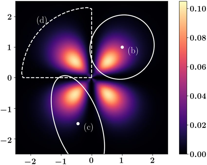
C. Maximum power
Although a global maximum for Pmax (∂ ) in Eq. (28)
is hard to find, it is still possible to design simple trajec-
tories with useful output power and reasonable efficiency.
We perform a numerical search of max∂ A2 /L2 using a
gradient-descent method, restricted to the space of elliptic
The trajectories (a),
trajectories centered at a given point B.
(b), and (c) shown in Fig. 3 are examples of the resulting
curves. We choose these types of curves because ellipti-
cal trajectories are easy to implement and flexible enough
to perform an extensive optimal search. The advantage of
Br(kBT ) the elliptical protocols is not obvious, taking into account
that Fig. 3 suggests that the circular-sector protocols are
FIG. 4. Positive eigenvalues of —see Eq. (33)—as a func- better than the ellipses for maximizing A. However, this is
tion of |B| = Br . Parameters are C = 120kB T and ¯ = 0.2 (solid not the case for A2 /L2 : we show in Appendix C that suit-
lines), ¯ = 0.05 (dashed lines). Note for ¯ = 0.2 (solid lines) able chosen ellipses can clearly outperform circular-sector
that most of the relevant region of Fig. 3 lies inside the interval protocols in terms of power output.
(Br,low , Br,high ) where the radial dissipation is about one order of Focusing on the elliptic protocols, we see that the high-
magnitude bigger than the polar dissipation. est values of power are achieved for test curves that avoid
where the dissipation coefficient λφ
the region of small |B|,
We see from the analytical expressions of Eqs. (35) diverges. The curve (a) centered at (0, 0) is an interesting
and (36) that is symmetric along the polar axis, i.e., it example. It maximizes A2 by enclosing the two lobes in
depends only on Br . This is illustrated in the upper panel the first and third quadrant of Fig. 3, and closes the curve
of Fig. 9 of Appendix B. In Fig. 4 we show the depen- near infinity in order to avoid the central region of high
dence of the coefficients λr and λφ on Br for two different dissipation.
values of the ¯ parameter. For some values of ¯ we find an In Fig. 5 we depict the value of max∂ A2 /L2 found by
interval (Br,low , Br,high ) for which the dissipation is mainly the mentioned heuristic method, as a function of the (fixed)
due to changes in the energy spectrum induced by finite central point of the ellipse. We distinguish two different
Ḃr . The specific values Br,low , Br,high depend on the work- regimes leading to the optimal power, as a consequence of
ing temperature and the coupling constant ¯ between the the crossover between the two mechanisms of dissipation
qubit and the reservoirs. More details on the submatrix discussed in the context of Fig. 4. For small Br , where the
and the dissipation structure of the qubit can be found in less dissipative protocol is radial, the optimal trajectories
Appendix B. are like the case (a) in Fig. 3, while in the opposite limit
The final value of L2 for a protocol B(θ τ ) defined over
∂ in the parameter space still depends on the chosen
parametrization θ. Out of all the possible parametrizations,
Eq. (15) tells us that there exists a particular one for which
L2 = L2 . Furthermore, this corresponds to the lower bound
for L2 and, importantly, it is a function of ∂ only (it is
geometrical).
In addition, for a given θ associated to ∂ , we are able
to obtain the optimal parametrization θ̄(θ) that saturates
the bound, and defines the less dissipative protocol B( θ̄ τ )
around ∂ in time τ . The new value of the velocity at a
given time can be computed using Eq. (15), demanding
˙
that B(θτ ˙ τ ) is constant at each point. The
· B(θ
) · (B)
result is
θ̄τ )
∂ B( ˙ L2
τ)
= B(θ , (41)
∂ θ̄ ˙ τ ) · (B)
B(θ ˙ τ )
· B(θ for a heuristic opti-
FIG. 5. max A2 /L2 as a function of B,
Parameters are
mization of elliptic trajectories centered at B.
where the dot in B˙ is the derivative with respect to the C = 120kB T and ¯ = 0.2. Only positive values of Bx and Bz are
original parametrization θ. This driving ensures constant shown, since this quantity is symmetric with respect to Bx = 0
entropy production along the cycle. and Bz = 0.
010326-8
GEOMETRIC OPTIMIZATION OF NONEQUILIBRIUM. . .                                                   PRX QUANTUM 3, 010326 (2022)

where Br is large, the optimal protocols are like the ones
indicated with (b) and (c) in that figure.

                   D. Maximum efficiency
   Following the same philosophy of the analysis of L2 pre-
sented in Fig. 4, we plot in Fig. 6 the maximum eigenvalue

                                                                         Bx(kBT )
of κ [defined in Eq. (30)] in order to visualize the value
of the thermal losses when the system evolves in the direc-
tion of maximum dissipation. Note that since κ(B)    is a
scalar, hence, an equivalent decomposition to Eq. (33) can
be done for 2κ as follows:

                   k   = λkr |rr| + λkφ |φφ|.              (42)

Furthermore the analysis presented for L2 in Sec. VI B, and                                        Bz(kBT )
particularly the results shown in Fig. 4 and Appendix B
still hold for the eigenvalues and eigenvectors of κ .                 FIG. 7. Maximum A2 /L2κ as a function of B for a heuristic
   In the case of the efficiency, an optimal solution is triv-                                                              Parameters are
                                                                       optimization of elliptic trajectories centered at B.
ially found by looking at Fig. 6 and considering again the                                ¯
                                                                       C = 120kB T and  = 0.2.
circular-sector curve (d) with  = π/2. From Eq. (38) we
see that along the Bx and Bz axis we have κ = 0, because
in those regions the system is coupled to only one of the                 In addition to this particular solution of special inter-
reservoirs. It is clear from Eq. (30) that for the limiting            est, we illustrate the usefulness of the method in a more
circular-sector protocol with R → ∞, enclosing the full                generic way. The strong equivalence between the geomet-
quadrant and leading to Eq. (39) we have κ = 0, which                rical quantities A2 /L2 and A2 /L2κ allows us to replicate the
implies x = ∞ in Eq. (21), hence ηmax = ηC . In fact, as               analysis done in the previous subsection in a straightfor-
already mentioned, this protocol is an equilibrium Carnot              ward manner. Once again, for a given a trajectory the value
cycle for the qubit, where the changes along the axis are the          of A2 is computed from Eq. (14) while the lower bound
isothermal compression and expansion. More details of the              for L2 κ and the corresponding optimal parametrization
efficiency of this protocol can be found in Appendix C.                  is given by Eq. (30) in complete analogy with Eqs. (15)
                                                                       and (41) from the maximum power analysis.
                                                                          We perform the numerical search of max∂ {A2 /L2κ }(B)
                                                                       again for the special case of closed elliptic curves cen-
                                                                       tered at a given point B. The computed result is presented
                                                                       in Fig. 7. In Fig. 6 we also show some of these trajec-
                                                                       tories, centered at the points B = {(1, 1), (−1.5, −0.45)}.
                                                                       Note that, while some differences can be spotted between
   Bx(kBT )

                                                                       these trajectories and the ones shown in Fig. 3, the quali-
                                                                       tative intuition is that efficient protocols are the ones with
                                                                       big A2 .

                                                                              E. The impact of optimizing the driving speed
                                                                          The aim of this section is to gather further insight on
                                                                       the effect of selecting the optimal protocol, regarding the
                                                                       trajectory ∂ and the optimal speed for the circulation on
                            Bz(kBT )
                                                                       the resulting power and efficiency of a heat engine.
                                                                          We consider an elliptical protocol for which we can
FIG. 6. Maximum eigenvalue of κ , indicating the losses due            define a “trivial” circulation with constant angular veloc-
to the combined effect of dissipation and thermal conduction.
                                                                       ity. For the case of the power, we compare the results of
Parameters are C = 120kB T and ¯ = 0.2. Curves (b),(c) are
heuristically searched protocols of elliptic shape, centered at        such trivial circulation with the one corresponding to the
(1, 1) and (−1.5, −0.45), respectively, that maximize the value        optimal velocity as defined in Eq. (41). For the case of
A2 /L2κ . Curve (d) (circular sector) is a quarter of circumference    the efficiency we compare the trivial circulation with the
centered at (0, 0), joined by two radial lines of length R along the   one corresponding to the optimal velocity, as defined in
axis.                                                                  Eq. (41) with the replacements L → Lκ and → κ .

                                                                010326-9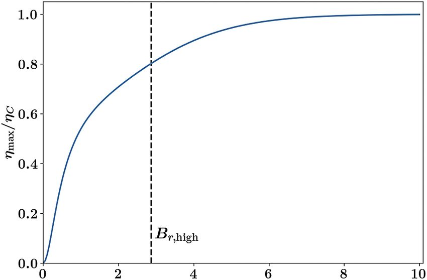
TERRÉN ALONSO, ABIUSO, PERARNAU-LLOBET, and ARRACHEA                                        PRX QUANTUM 3, 010326 (2022)

                                                                        It is interesting to compare the value obtained for the
                                                                     maximum power in the protocol under consideration with
                                                                     the power associated to the limiting value for the work
                                                                     given by Eq. (39). Such limiting power can be obtained by
                                                                     replacing τP of Eq. (18) in Eq. (12), where we see that at
                                                                     finite time the net work done by the machine operating at
                                                                     maximum power is WPmax = AηC /2. Taking into account
                                                                     that for the heat engine A ≤ log(2)kB T—see Eq. (39)—we
                                                                     conclude that the bound for the maximum operating power
                                                                     in a cycle of duration τP is Plim = log(2)kB T ηC /(2τP ). For
                                                                     the case of the protocol (b), given the values of Eq. (43),
                                                                     we get Pmax = 0.7Plim .
FIG. 8. Power (blue) and efficiency (orange) for curve (b) of
                                                                        In a similar way using Eq. (21), the optimized
Fig. 6 as a function of the cycle duration τ . Solid lines: cir-     parametrization that maximizes the efficiency of the cycle
culating around the curve at constant angular velocity. Dashed       gives us the value ηmax = 0.34ηC .
lines: using the optimal velocities given by Eqs. (15) (for power)      Specific values for the maximum efficiency of the
and (30) (for efficiency).                                             machine operating under other protocols can be obtained
                                                                     by substituting in Eq. (22) the values shown in Fig. 7. This
   For the sake of concreteness, we focus on ∂ given by              calculation shows that this machine can achieve a perfor-
the protocol (b) of Fig. 3. Results are shown in Fig. 8,             mance as high as ηmax > 0.55ηC . These results are very
where we show the power and efficiency of the machine                  encouraging regarding the possibility of the experimental
as a function of the cycle total duration. Plots in solid            implementation of this system.
and dashed lines correspond, respectively, to the proto-
cols with constant angular velocity and optimal velocity.                    VII. SUMMARY AND CONCLUSIONS
We note from this figure that the optimized parametriza-
tion is around 2 times bigger in power, and around 4 times              We have followed a geometrical approach to describe
more efficient, with respect to the trivial parametrization of         the two competing mechanisms of a nonequilibrium adi-
the ellipse circulated at a constant angular velocity. Dashed        abatic thermal machine: the dissipation of energy and
lines in Fig. 8 are akin to those of Fig. 2 where power val-         the heat-work conversion. While the first mechanism is
ues are normalized to Pmax and efficiencies to ηmax , and              described in terms of a length, the second one can be repre-
summarizes the performance of the machine.                           sented by and area in the parameter space. We then showed
                                                                     that the problem of finding optimal protocols reduces to an
             F. Estimates for the performance                        isoperimetric problem, which consists in finding the opti-
                                                                     mal ratio between area and length in a space with nontrivial
   To finalize the analysis of the qubit heat engine, it is           metrics.
interesting to analyze concrete values characterizing its               We applied this description to a thermal machine, which
performance. As before, we focus on the protocol (b) of              consists of a single qubit asymmetrically coupled to two
Fig. 3, for which we have                                            bosonic reservoirs at small different temperatures and
                                                                     driven by a cyclic protocol controlled by two parame-
               A2 = 0.233kB2 T2     L2 = 7.71.              (43)    ters that vary slowly in time. We solved this problem
                                                                     in the limit of weak coupling between the qubit and the
For these values, we find using Eq. (20):
                                                                     reservoirs. We analytically show the limiting value of the
                                       pW                            pumped heat between reservoirs is given by Landauer
            Pmax = 1.364 × 10⁻²           (T)2 ,                    bound in an ideal Carnot cycle. We analyzed in this prob-
                                       K2
                                                                     lem the type of cycles leading to optimal performance of
which for a working temperature of T = 100 mK and                    the machine. Interestingly, the qubit machine has a very
a temperature bias corresponding to T = 0.05 T, as in               good ratio between performance and power within a wide
previous figures, gives Pmax = 0.341 aW with efficiency                 set of parameters.
ηPmax = 0.23ηC . The total time τP for maximum power                    According to our analysis, efficiencies larger than 0.55
output per cycle is computed through Eq. (19):                       of the Carnot cycle can be achieved and values of the
                                                                     corresponding output power of 0.7 of the limiting power,
                     τP = 2τD = 48.8 ns,                             corresponding to the work done in an ideal Carnot cycle
                                                                     divided by the duration of the cycle at which the maximum
which corresponds to an operation frequency in the order             power is achieved. These estimates are very encouraging
of 0.1 GHz.                                                          for the experimental implementation of this machine. In

                                                              010326-10
GEOMETRIC OPTIMIZATION OF NONEQUILIBRIUM. . . PRX QUANTUM 3, 010326 (2022)
this sense, a very promising platform is a superconduct- 1. Reduced density matrix
ing qubit coupled to resonators, in which there have been The Hamiltonian for the qubit can be expressed, after an
several configurations under study for some years now appropriate unitary transformation U, in the instantaneous
[73–78]. Other possible platforms are those in which the diagonal basis |j , j = 1, 2 as follows:
Otto cycle has been already implemented, like AMO sys-
tems [2,79,80], as well as spin systems in NMR setups [6]. Hqb (t) = E1 (t)|11| + E2 (t)|22|, (A1)
Quantum dots, where electron pumping has been observed
[81,82], are also candidates for implementing the heat where E1,2 (t) = ∓Br (t) are the eigenvalues of the Hamil-
engine and refrigerator operations as well as nanomechan- tonian of Eq. (32). We focus on the reduced density matrix
ical systems [83,84]. This geometrical optimization can ρ(t) expressed in this basis, in the slow-driving regime. We
also be very naturally extended to analyze other systems split it into a frozen plus an adiabatic contribution as
like motors operating under slow driving and a bias volt-
age [85–88]. In the present work, we have focused on the ρ(t) = ρ f + ρ a , (A2)
linear-response regime, where the geometric description
becomes explicit. The weak-coupling calculations of the where the first term corresponds to the description with the
heat and work presented in Sec. VI and Appendix A 1 can Hamiltonian frozen at a given time, for which the parame-
be extended to analyze the operation beyond this regime ters take values B, while the second one corresponds to the
for specific thermal machines, representing an outlook to correction ∝ dt B.
further works. The master equation for the corresponding matrix ele-
ments, ρij (t), reads [71]
ACKNOWLEDGMENTS
dρij (t) iij (t) jn
We thank Rosario Fazio and Jukka Pekola for stimulat- = ρij + Mmi,α (t)ρmn + Mjm,α
in
(t)ρnm
dt h m,n,α
ing discussions. P.A. is supported by “la Caixa” Founda-
tion (ID 100010434, Grant No. LCF/BQ/DI19/11730023),
− Mjm,αmn
(t)ρin − Mmi,α
mn
(t)ρnj , (A3)
and by the Government of Spain (FIS2020-TRANQI
and Severo Ochoa CEX2019-000910-S), Fundacio Cellex,
Fundacio Mir-Puig, Generalitat de Catalunya (CERCA, where we introduce a shorthand notation for Ei (t) −
AGAUR SGR 1381). L.A. and P.T.A. are supported by Ej (t) = ij (t) for the instantaneous energy differences.
ju
CONICET, and acknowledge financial support from PIP- The transition rates Mml,α (t) for the present problem are
2015 and ANPCyT, Argentina, through PICT-2017-2726, given by
PICT-2018-04536. L.A. thanks KITP for the hospitality
ju ξα,ml (t)ξα,ju (t)
in the framework of the activity “Energy and Informa- Mml,α (t) = {nα (ju )α (ju )
tion Transport in nonequilibrium Quantum Systems” and h
the support by the National Science Foundation under + [1 + nα (uj )](uj )}, (A4)
Grant No. PHY-1748958, and the Alexander von Hum-
boldt Foundation, Germany. M.P.-L. acknowledges fund- α ε/(k
= h, c being
the reservoir indices, nα (ε) = 1/
ing from Swiss National Science Foundation through an e B Tα ) − 1 the Bose-Einstein distribution function cor-
Ambizione Grant No. PZ00P2-186067. responding to the temperature of the α reservoir, and
α (ε > 0) = γα εe−ε/εC the bath spectral function. The
APPENDIX A: CALCULATION OF THE functions ξα are defined for each bath as ξα = Û(t)π̂α Û† (t),
LINEAR-RESPONSE COEFFICIENTS where πα is defined in Eq. (3). In the present problem
we use π̂h,c = σ̂x,z . For this problem we consider Ohmic
In what follows we calculate all the linear-response baths with a cutoff frequency εC , and α (ε ≤ 0) = 0. The
coefficients entering Eqs. (6) and (7) in the weak-coupling value of γα depends on the coupling strength as |Vα |2 . This
limit between the qubit and the reservoir, following quantity defines the relaxation time between the q-bit and
Ref. [71]. We rely on the adiabatic quantum-master the reservoirs, τrel ∝ γα−1 ε ≈ γα−1 kB T. In Eq. (A3) we have
equation approach under small temperature bias T to [71,89–91].
neglected a term proportional to |Vα |2 |dt B|
evaluate the coefficients μ,ν , which enable the calcula-
This equation can be written in a compact form as
tion of the net transferred heat and work defined in Eqs. (6)
and (7). dp(t)
The derivation of the master equation corresponds to = M(t)p(t), (A5)
dt
solving the nonequilibrium problem of the driven qubit
coupled to the two reservoirs exactly up to second order by defining p(t) = [ρ11 (t), ρ12 (t), ρ21 (t), ρ22 (t)]T with the
in the coupling constants V2α and up to linear order in the contributions pf and pa as in Eq. (A2) and M(t)
velocities of the driving parameters dt B. accordingly.
010326-11TERRÉN ALONSO, ABIUSO, PERARNAU-LLOBET, and ARRACHEA PRX QUANTUM 3, 010326 (2022)
The frozen contribution pf is calculated as a function In order to discriminate the contribution of the devel-
of the time-dependent parameters B only (frozen time), oped power ∝ T, and recalling that we are considering
and satisfies the stationary (static) limit [dpf (t)/dt] = 0. small temperature differences, we introduce the follow-
f
Hence, it can be calculated from ing extra expansion in frozen component: ρ f = ρT +
δT ρ f T. Therefore,
0 = M(B)
· pf (B), (A6)
∂ Hqb
with the normalization condition +
f
= 1. On the
ρ11
f
ρ22 = −Tr
,3 (B) δT ρ f , (A12)
other hand, the adiabatic component satisfies ∂B
∂pf (B)
while
· pa (t),
Ḃ (t) = M(B) (A7)
∂B
∂ Hqb ∂pf T
with the normalization condition ρ11
a
+ ρ22
= 0. An impor-
a = [ ],n (B)
,n (B) = Tr M̃−1
T (B) ,
∂B ∂Bn
tant detail for the calculation of the partial derivatives
(A13)
appearing in the left side of Eq. (A7) is to take into account
the effects of the basis dependence in B. A practical way to
perform the derivative is by expressing ρ f in the laboratory where we highlight with the subindex T that the quantities
(fixed) basis first, and then rotate back to the instantaneous are calculated with the reservoirs at the same temperature
diagonal basis. T and the quantity between parentheses is to be under-
We can modify M to include the normalization condi- stood as a 2 × 2 matrix. Notice that the contribution of
tion for pa in a single equation [90,91]. Naming M̃ the f
Eq. (A9) evaluated with ρT corresponds to an equilibrium
resulting matrix, we can finally invert Eq. (A7) to obtain quantity. It represents the power developed by the conser-
the closed expression vative ac forces, and it, thus, leads to a vanishing value
when averaged over the cycle.
∂pf In the same formalism used to derive the reduced density
pa (t) = ·
M̃−1 (B) Ḃn (t). (A8)
n
∂Bn matrix, the heat current entering the reservoir α, calcu-
lated at the second order of perturbation theory in the
2. Linear-response coefficients coupling to the reservoirs and within the adiabatic regime,
reads [71,91]
We can now use the described approach in Appendix (A 1)
to obtain explicit expressions for the linear-response coef- nu
ficients entering in the thermal geometric tensor μ,ν . Jα (t) = un (t)Re Mmn,α (t)ρun (t) . (A14)
To this end, we calculate the power developed by the m,n,u
ac-driving sources as follows:
We can follow the same logic as before to calculate this
Pac (t) = Tr Ḣqb (t)ρ(t) , (A9)
˙ The first one is “ther-
current at the first order in T and B.
being mal” component associated to the the frozen components
evaluated with a thermal bias T, while the second one
∂ Hqb (t) is the heat current “pumped” by the ac driving without
Ḣqb (t) = Ḃ (t). (A10) temperature bias.
∂B
The linear-response net transported heat between the
two reservoirs is
We now write
τ τ τ
W=− dtPac (t), (A11) Q= dtJc (t) = − dtJh (t). (A15)
0 0 0
and replace Eq. (A2) into Eq. (A9), to finally use the solu-
tions for pf and pa obtained in the previous subsection. We follow the convention of Ref. [15] and consistently
The resulting expression can be directly compared to the with the definition (7), we focus on the current entering the
formal relation in Eq. (6) for W, where the matrix elements cold reservoir to define the net transported heat. Associat-
of the thermal geometric tensor are multiplied by different ing each term of Eq. (7) with those arising from Eq. (A14)
powers of Ḃk . upon substituting ρ by its expansion in T and B, ˙ we
010326-12GEOMETRIC OPTIMIZATION OF NONEQUILIBRIUM. . . PRX QUANTUM 3, 010326 (2022)
identify the linear coefficients, because the eigenvectors |i are associated to the unitary
transformation that makes Hqb diagonal, and do not change
= (B)
=
∂pf when B stays in the same direction.
3, (B) un Re Mmn,c,T
nu
M̃−1
m,n,u
T
∂B un
These facts allows us to separate the linear-response
coefficient into a radial contribution λr (changes in the
(A16)
energy spectrum) and a polar contribution λφ (basis rota-
tion). Inserting the solution to Eqs. (A6) and (A8) into
and
Eq. (A13) we get
κ(B) nu
3,3 (B) = = um Re Mmn,c,T δT ρ f un . (A17)
T =
βsinh(βBr )
m,n,u r| |r = λr (B) , (B4)
(2Br )cosh3 (βBr )
These coefficients satisfy the following Onsager equations
=
(2Br )
[15,63], φ| |φ = λφ (B) . (B5)
4Br3
3, =− ,3 , 1,2 = 2,1 . (A18)
Equation (A13) finally reads
APPENDIX B: EXPLICIT EXPRESSIONS FOR
(
(B), B),
AND κ(B)
IN THE CASE OF EQUAL = λr |rr| + λφ |φφ|. (B6)
BATH COUPLING
Assuming equal spectral density in the L and R baths, We now turn to analyze L2 , which quantifies the dis-
i.e., sipated energy for a particular protocol, determined by
through Eq. (11). In the upper panel of Fig. 9 we
L () = ¯ L e−/C = (), show the maximum eigenvalue, max λr , λφ as a func-
(B1)
R () = ¯ R e−/C = (), tion of (Bz , Bx ). This plot reflects the behavior resulting
from the analytical expressions of Eqs. (B4) and (B5).
with ¯ L = ¯ R constants, we get explicit expressions At every point, and depending on the values of ¯ and T,
for the complete geometric tensor. Using (Bx , Bz ) = this maximum eigenvalue corresponds to a pure polar or
pure radial displacement of B. Within the small circle plot-
Br (sin φ, cos φ) and β = 1/(kB T) we arrive to the follow-
ing results. ted in dashed lines and outside the one in solid lines, the
highest eigenvalue is λφ , while within the two circles, λr
is the largest one. This means that for small Br < Br,low
1. Explicit expression for
as well as for large Br > Br,high , protocols leading to the
Using Eq. (A1) and the expression for the reduced den- smallest dissipation are those associated to changes in
sity matrix in the same basis, we can write for the terms Br , while for Br,low < Br < Br,high , protocols associated to
with partial derivatives in Eq. (A13): rotations are the least dissipative ones. The specific values
Br,low , Br,high depend on the temperature and the coupling
∂ Hqb
= j | + Ej (B)(|∂
∂ Ej (B)|j j j | + |j ∂ j |), between the qubit and the reservoirs, as shown in Fig. 4
∂B j
for two values of .
(B2) The precise shape of the interval Br,low , Br,high is shown
in the lower panel of Fig. 9 and depends only on , ¯ while
∂pf T
=
f
∂ pT,ij (B)|ij
f ij | + |i∂ j |),
| + pT,ij (B)(|∂ the final value has a linear dependence on kB T. We see
∂Bn ij
that for ¯ 0.6 the rotational dissipation dominates for
all values of |B|.
(B3)
with the notation ∂/∂B = ∂ . We note that the term Ej (B) and κ
2. Explicit expression for
depends only on the absolute value of the magnetic field
f Again, plugging the expressions describing p(t) given
Br . In addition, the density matrix pT (B) is a function of
by Eqs. (A6) and (A8) into Eq. (A16) we get for the qbit:
the energy spectrum, since it is computed in thermal equi-
librium considering both baths at equal temperature T, and
thus depends only on Br as well. 1 (B)
= −βBr sin3 (φ)sech2 (βBr ), (B7)
On the other hand, the operators |∂ ij | and |i∂ j |
2 (B)
= −βBr sin (φ) cos(φ)sech (βBr ).
2 2
(B8)
are nonzero only for variations in the polar coordinate φ
010326-13You can also read