Fuzzy Cognitive Maps with Bird Swarm Intelligence Optimization-Based Remote Sensing Image Classification

Hindawi
Computational Intelligence and Neuroscience
Volume 2022, Article ID 4063354, 12 pages
https://doi.org/10.1155/2022/4063354

Research Article
Fuzzy Cognitive Maps with Bird Swarm Intelligence
Optimization-Based Remote Sensing Image Classification

 Anwer Mustafa Hilal ,1 Hadeel Alsolai,2 Fahd N. Al-Wesabi ,3 Mohamed K Nour,4
 Abdelwahed Motwakel,1 Anil Kumar ,5 Ishfaq Yaseen,1 and Abu Sarwar Zamani1
 1
 Department of Computer and Self Development, Preparatory Year Deanship, Prince Sattam Bin Abdulaziz University,
 AlKharj, Saudi Arabia
 2
 Department of Information Systems, College of Computer and Information Sciences,
 Princess Nourah Bint Abdulrahman University, P.O. Box 84428, Riyadh 11671, Saudi Arabia
 3
 Department of Computer Science, College of Science & Art, Mahayil, King Khalid University, Saudi Arabia
 4
 Department of Computer Science, College of Computing and Information System, Umm Al-Qura University, Saudi Arabia
 5
 Data Science Research Group, School of Computing, DIT University, Dehradun, India

 Correspondence should be addressed to Anwer Mustafa Hilal; a.hilal@psau.edu.sa

 Received 15 January 2022; Revised 13 February 2022; Accepted 23 February 2022; Published 27 March 2022

 Academic Editor: Diego Oliva

 Copyright © 2022 Anwer Mustafa Hilal et al. This is an open access article distributed under the Creative Commons Attribution
 License, which permits unrestricted use, distribution, and reproduction in any medium, provided the original work is
 properly cited.
 Remote sensing image (RSI) scene classification has become a hot research topic due to its applicability in different domains such
 as object recognition, land use classification, image retrieval, and surveillance. During RSI classification process, a class label will
 be allocated to every scene class based on the semantic details, which is significant in real-time applications such as mineral
 exploration, forestry, vegetation, weather, and oceanography. Deep learning (DL) approaches, particularly the convolutional
 neural network (CNN), have shown enhanced outcomes on the RSI classification process owing to the significant aspect of feature
 learning as well as reasoning. In this aspect, this study develops fuzzy cognitive maps with a bird swarm optimization-based RSI
 classification (FCMBS-RSIC) model. The proposed FCMBS-RSIC technique inherits the advantages of fuzzy logic (FL) and
 swarms intelligence (SI) concepts. In order to transform the RSI into a compatible format, preprocessing is carried out. Besides,
 the features are produced by the use of the RetinaNet model. Besides, a FCM-based classifier is involved to allocate proper class
 labels to the RSIs and the classification performance can be improved by the design of bird swarm algorithm (BSA). The
 performance validation of the FCMBS-RSIC technique takes place using benchmark open access datasets, and the experimental
 results reported the enhanced outcomes of the FCMBS-RSIC technique over its state-of-the-art approaches.

1. Introduction scene patches based on its content, has become a hot topic in
 the fields of RSI interpretation due to its crucial application
With the advancement of Earth observation techniques, in land resource management, LULC, disaster monitoring,
several kinds (for example, multi/hyperspectral and syn- traffic control, and urban planning [2]. In recent times,
thetic aperture radar) of higher-resolution images of Earth’s various approaches were introduced for RSI scene classifi-
surface are easily accessible [1]. Hence, it is highly significant cation [3].
to efficiently understand the semantic content, and more The earlier method for scene classification have been
intelligent classification and identification techniques of land largely dependent on lower-level or handcrafted features
use and land cover (LULC) are certainly required. Remote that aims at developing different human-engineering feature
sensing image (RSI) scene classification, which intends to globally or locally, namely, texture, color, spatial, and shape
automatically assign a certain semantic label to all the RSI data. A typical feature includes the color histogram (CH),

2 Computational Intelligence and Neuroscience

scale invariant feature transform (SIFT), Gabor filters, local classification outcome. Shawky and others [11] presented an
binary pattern (LBP), the histogram of oriented gradient effectual classification approach named CNN-MLP to use
(HOG), and gray level co-occurrence matrix (GLCM) are the merits of these 2 approaches: CNN and MLP. The feature
widely employed for scene classification [4]. It is noteworthy is created by utilizing the pretrained CNN without a FC
that methods based on this lower-level feature performed layer.
effectively on image with spatial arrangements or uniform Li and others [12] introduced an RSSC-based error-
texture, but still, they are constrained to distinguish images tolerant deep learning (RSSC-ETDL) method for miti-
with more complex and challenging scenes, that is because gating the negative effects of incorrect labels of the RSI
the contribution of human in feature design considerably scene datasets. In the presented approach, correcting error
influence the efficiency of the representative capability of labels and learning multiview CNNs are simultaneously
scene image [5]. In comparison with the lower-level feature- performed in an iterative method. It should be noticed that
based method, the midlevel feature approach attempts to to generate the alternate system perform efficiently, we
calculate a holistic image representation generated by local present an adoptive multifeature collaborative represen-
visual features including color histogram, SIFT, or LBP of tation classification (AMF-CRC) which benefited from
the local image patch [6]. adoptively integrating various features of CNN for cor-
 The common pipeline of constructing midlevel features recting the label of undefined sample. Xu and others [13]
is to extract local attributes of image patches initially and presented a classification model including RNN and RF for
later for encoding them to attain the midlevel representation land classification with a satellite image that is open source
of RSI. The bag-of-visual-words (BoVW) method is one of for different study objectives. Then, the study utilized
the common midlevel methods and is broadly adapted for spatial data collected from the satellite image (that is time
RSI scene classification due to its effectiveness and simplicity series).
[7]. The method based on BoVW has enhanced performance Min and others [14] developed an approach called deep
of the classification; however, because of the limitations of combinative feature learning (DCFL) for extracting lower-
representative ability of BOVW method, no other break- level texture and higher-level semantic data from various
through has been accomplished for RSI scene classification. network layers. First, feature encoder VGGNet-16 is fine-
Recently, the deep learning (DL) method is commonly tuned for succeeding multiscale feature extraction. Then,
utilized in several image processes [8]. From the deep-re- two shallow convolutions (Conv) layers are carefully chosen
stricted Boltzmann machines (DBM) and deep confidence for convolution feature summing maps (CFSM), where we
networks (DBN) to deep convolution neural networks extract uniform LBP with rotation invariance for excavating
(CNN), significant improvement has been attained in dis- comprehensive texture. A deep semantic feature from the FC
tinct image fields. Particularly, CNN is acknowledged as one layer concatenated with shallow feature constitutes deep
of the common techniques because of the capacity to learn combination feature that is thrown into SVM classification
hierarchical level abstraction of input data by encoded input for last classification.
data on distinct layers [2, 9]. In contrast to the conventional Huang and others [15] presented a task-adoptive
model, CNN approach has accomplished effective classifi- embedding network for facilitating few-shot scene clas-
cation accuracy. sification of RSI, represented as TAE-Net. First, a feature
 This study develops fuzzy cognitive maps with bird encoder was trained on the base set for learning embedded
swarm optimization based RSI classification (FCMBS-RSIC) features of input image in the pretraining stage. Next, in
model. The proposed FCMBS-RSIC technique inherits the the meta-training stage, a task-adoptive attention method
advantages of fuzzy logic (FL) and swarms intelligence (SI) was developed for producing the task-specific attention
concepts. In order to transform the RSI into a compatible that could adoptively choose embedding features amongst
format, pre-processing is carried out. Besides, the features the entire task. Yin and others [16] examined the fusion-
are produced by the use of the RetinaNet model. Besides, a based model for RSI scene classification from other
FCM-based classifier is involved to allocate proper class viewpoints. First, it is classified into front, middle, and
labels to the RSIs and the classification performance is back side fusion modes. For every fusion mode, the cor-
enhanced by the design of bird swarm algorithm (BSA). The related method is described and introduced. Next, clas-
performance validation of the FCMBS-RSIC technique takes sification performance of the single and hybrid side fusion
place using benchmark open access datasets. modes is estimated.

2. Related Works 3. Proposed Model
Zhang and others [10] presented an efficient RSI scene In this study, a new FCMBS-RSIC approach was developed
classification framework called CNN-CapsNet for using the for the detection and classification of RSIs. The proposed
advantages of these 2 techniques: CapsNet and CNN. First, a FCMBS-RSIC method encompasses distinct subprocesses
CNN without the FC layer is utilized as first feature map such as pre-processing, RetinaNet-based feature extraction,
extractor. Particularly, a pretrained D-CNN method that has FCM-based classification, and BSA-based parameter tuning.
been completely trained on the ImageNet data set is carefully The design of BSA helps to properly tune the parameters
chosen as a feature extractor. Next, the first feature map is involved in the FCM model, and consequently, the classi-
given to a recently developed CapsNet to attain the last fication efficiency can be improved.

Computational Intelligence and Neuroscience 3

3.1. Preprocessing. Primarily, image pre-processing is car- FPN and then integrate for creating the last feature output
ried out to make it compatible with further processes. Since combinations. The class subnet from the FCN carried out the
the images are in the RGB format, they are transformed into classification task. This subnet is recognized that view the
grayscale versions. Besides, the unwanted portions of the echocardiography image appears to. The box subnet from
images that are considered to be unwanted are removed. The the FCN carried out the border regression tasks. Its role is for
images are filtered by the use of digital filters to get rid of the detecting the place of left ventricle from the echocardiog-
noise and discrepancies. raphy image and recording the co-ordinate. Figure 1
 demonstrates the framework of RetinaNet.
 Focal loss: the focal loss is an enhanced form of cross
3.2. Feature Extraction: RetinaNet Model. At the time of entropy (CE) loss, and the binary CE expression is as follows:
feature extraction, the FCMBS-RSIC technique derives the
feature vectors using the RetinaNet model. The CNNs are − log (p), if y � 1,
 CE(p, y) � (3)
developed in an order of layers. An input map is stimulated − log (1 − p), otherwise,
with the individual’s layer still achieving the resultant map
[11]. Detailed individual layers are provided to demonstrate where y ∈ [ ± , 1] signifies the ground truth type and
of computation equation. Let X ∈ Rh×w×c (h): height, w: p ∈ [0, 1] indicates the forecast probabilities of model to
width, c: channel) are RGB images. All the layers get X and type y � 1.
the group of parameters W as input and output a novel p, if y � 1,
image y ∈ Rh′ ×w′ ×c′ , for instance, y � f(X, W). pt � (4)
 Primary, a convolution layer is an essential layer of the 1 − p, otherwise.
CNN. The learnable filter signifies the parameter of this layer The previous equation is abbreviated as follows:
sliding the filters on every input volume with existing width
as well as height. This creates an activation map signifying CE(p, y) � CE pt 
 (5)
the reaction of that filter at all spatial regions. In order to � − log pt .
compute the convolutional of input X with bank of filters
W ∈ Rhxw×c×c′ and adding a bias ∈∈Rc′ , equation (1) was For solving the issue of data imbalance amongst the
utilized. positive as well as negative instances, the novel procedure
 h w c
 was altered as to the subsequent method:
 ⎝b ′ + W
 yi′ j′ k′ � f⎛ ⎠
 ⎞ (1)
 k ij dk × Xi′ +i, j′ +j,d′ . CE pt � −αt log pt . (6)
 i�1 j�1 d�1
 Amongst them,
 Second, the max-pooling layer was utilized for de-
creasing the parameter and computation from the network α, if y � 1,
 αt � (7)
with decreasing the size of imputing shapes. It calculates the l − α, otherwise,
maximal response of all image channels from h × w sub
window that performs as subsampling function. It is for- where α ∈ [0, 1] refers the weight factors. For solving the
mulated as follows: issue of complex instance, the concentrating parameter C
 was established for obtaining the last procedure of focal loss:
 yi′ j′ k′ � max, 1 < j < w Xi′ +ij′ +j, k . (2) c
 1

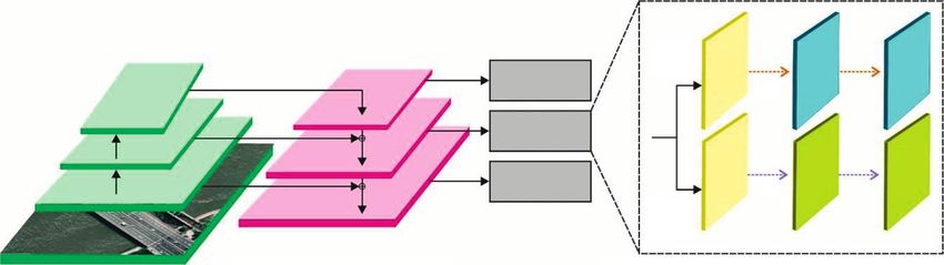
4 Computational Intelligence and Neuroscience

 Class
 W×H W×H W×H
 Class+Box Subnet
 ×256 ×4 ×256 ×256
 Subnets
 Class+Box
 Subnets
 W×H W×H W×H
 Class+Box
 ×256 ×4 ×256 ×256
 Subnets
 Box
 Subnet

 (a) ResNet (b) Feature Pyramid Net (c) Class Subnet (top) (d) Box Subnet (bottom)
 Figure 1: Structure of RetinaNet [17].

 (i) When wij > 0, a rise (decrement) in the cause Ci M
 produces an increment (decrement) of the impact A(t+1)
 i
 ⎝ w 2A(t) − 1 + 2A(t) − 1 ⎞
 � f⎛ ji j i
 ⎠, i ≠ j. (12)
 Cj with intensity |wij |. j�1

 (ii) When wij < 0, a rise (decrement) in the cause Ci When the cognitive network is capable of converging,
 produces a decrement (increment) of the neuron Cj the scheme would generate the similar output, and then the
 with intensity |wij |. activation degree of neuron remains unchanged. At the same
 (iii) When wij � 0, there are no causal relations among time, a cyclic FCM generates different responses with the
 Ci and Cj . This rule is iterated till an ending cri- exception of some state that is regularly generated. The final
 terion is satisfied. A new activation vector is esti- potential scenarios are associated with chaotic configuration
 mated at every step t and afterward a fixed amount where the network produces distinct state vectors.
 of iterations. The FCM is stated to have converged
 when it reaches fixed-point attractors or else the
 update procedure stops afterward a maximal 3.4. Parameter Optimization: Bird Swarm Algorithm. In
 amount of iterations T is attained. order to optimally adjust the parameters involved in the
 FCM technique, the BSA is applied to it. BSA, presented by
 Meng and others [19], is a novel intelligent bionic technique
 M dependent upon multigroup and multisearch techniques; it
 A(t+1) ⎝ w A(t) ⎞
 � f⎛ ⎠, i ≠ j. (9) simulates the birds foraging performance, vigilance per-
 i ji j
 j�1 formance, and flight performance, and utilizes this SI for
 solving the optimized issue. The bird’s swarm technique was
 The function f(·) signifies a monotonically nonre- based on 5 rules:
ducing nonlinear function utilized for clamping the ac-
tivation values of all the neurons to the interval. An Rule 1. All the birds are switching amongst vigilant as well
instance of this function is the sigmoid variants, bivalent as foraging performance, and combined bird forage and
function, and trivalent function. Then, attention is drawn keep vigilance are simulated as arbitrary decisions.
toward the sigmoid function because it has displayed
greater predictive abilities A nonlinear transfer function is Rule 2. if the foraging, all birds recorded and updated their
utilized in the study, whereas λ represents the sigmoid preceding optimum knowledge and swarm prior optimum
slope and h indicates the offset. Various researches have skill with food patch. The skill is also be utilized for searching
revealed that this parameter is tightly linked to network for food. Instant sharing of social data was through the
convergence. group.
 1
 f Ai � . (10)
 1+e − λ( A i − h ) Rule 3. Once they keep vigilance, all birds attempts for
 This rule is chosen while upgrading the activation value moving near the center of swarms. It is performance may be
of neuron which is not impacted by neural processing entity. controlled by disturbance due to swarm competition. The
 bird with further stocks was highly possible toward swarm
 M
 ⎝ w A(t) + A(t) ⎞
 ⎠, i ≠ j. centers than bird with lease stock.
 A(t+1)
 i � f⎛ ji j i (11)
 j�1
 Rule 4. The bird flies to another location frequently. If flying
 The alternative adapted upgrading rule has been presented to another place, birds frequently switch amongst produc-
for avoiding the conflict that emerges in the event of nonactive tion as well as shrub. The bird with maximum stocks are
neuron. More apparently, the rescaled inference permits producers, and bird with minimum is scrounger. Another
handling the scenario while there are no data regarding a first bird with maximal and minimal reserves is arbitrarily chosen
neuron state and assist to prevent the saturation issue. to producer and scrounger.

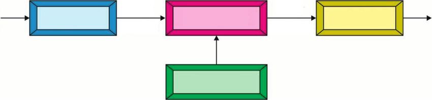
Computational Intelligence and Neuroscience 5

 Crisp Fuzzy Fuzzy Crisp
 Fuzzifier Intelligence Defuzzifier
 Input Input Set Output Set Output

 Rules

 Figure 2: Process of fuzzy logic.

 Figure 3: Sample images UCM21 dataset.

Rule 5. Producer actively seeks food. The scroungers arbi- xt+1 t t t
 i,j � xi,j + A1 meanj − xi,j × rand(0, 1)
trarily follow producers searching for food.
 Based on Rule 1, it can be determined that the time
 + A2 ptk,j − xti,j × rand (−1, 1),
interval of all birds flight performance FQ, the probabilities
of foraging performance P(P ∈ (0, 1 and uniform arbitrary (14)
 pFiti
number δ ∈ (0, 1))). A1 � a1 × exp − × N ,
 When the amount of iteration was lesser than FQ and sumFit + ε
δ ≤ P, the bird was foraging performance. Rule 2 is for- pFiti − pFitk N × pFitk
mulated mathematically as follows: A2 � a2 × exp × ,
 pFitk − pFiti + ε sumFit + ε
xt+1 t t t t t
 i,j � xi,j + pi,j − xi,j × C × rand (0, 1) + gj − xi,j 
 (13)
 × S × rand (0, 1), where a1 and a2 denotes the 2 positive constants from zero and
 two, pFiti indicates the optimum fitness value of ith bird and
where C and S are 2 positive numbers; the previous is named sumFit refers to the sum of swarms’ optimum fitness value. At
as the cognitive accelerated co-efficient, and the final is this point, ε that are utilized for avoiding zero-division error is
named as the social accelerated co-efficient. At this point, pi,j the minimum constant from the computer. meanj stands for
represents the ith bird optimum preceding place and gj the jth element of entire swarm’s average place.
signifies the optimum previous swarm place [20]. When the amount of iteration is equivalent FQ, the bird
 When the amount of iteration is lesser than FQ and is flight performance that is separated as to performance of
δ > P, the bird is vigilance performance. The Rule 3 is for- producer and scrounger by fitness. Rule 3 and Rule 4 are
mulated mathematically as follows: formulated mathematically as

6 Computational Intelligence and Neuroscience

 Figure 4: Sample images AID dataset.

 Figure 5: Preprocessed images.

 xt+1 t t The BSA approach derives a FF for reaching increased
 i,j � xi,j + randn (0, 1) × xi,j ,
 (15) classification efficiency. It resolves a positive integer for rep-
 xt+1 t t t
 i,j � xi,j + xk,j − xi,j × FL × rand (0, 1), resenting the optimum efficiency of the candidate solution.
 During this case, the minimized classifier error rate was assumed
where FL (FL ∈ [0, 2]) demonstrates that the scrounger is that FF is provided in equation (16). The optimal result is a lower
follow the producers for searching for food. error rate and worst solution gains an enhanced error rate.

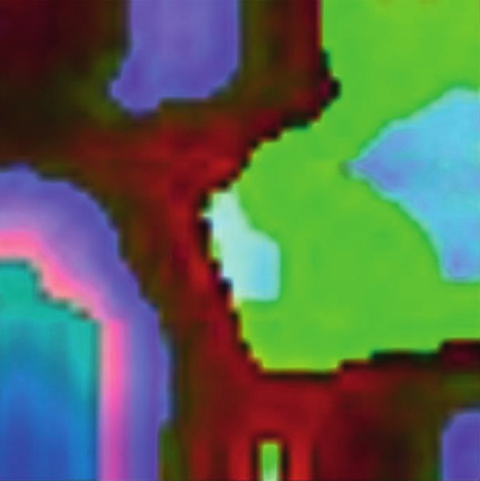
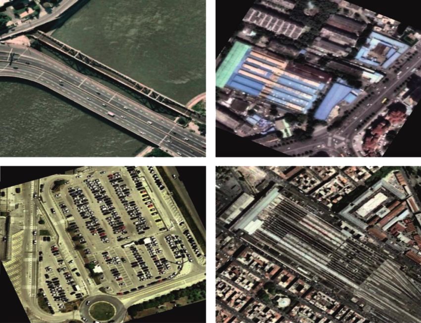
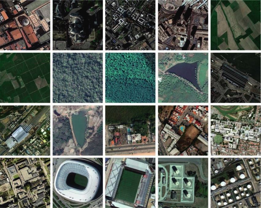
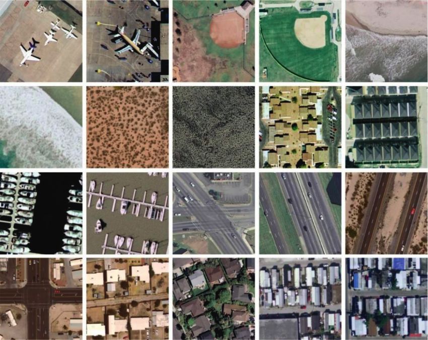
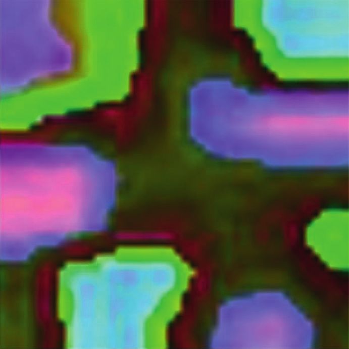
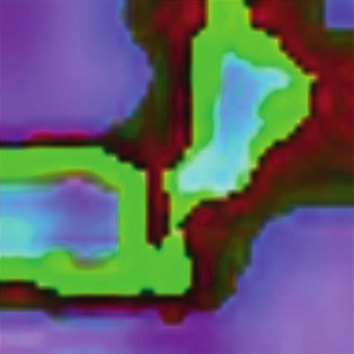
Computational Intelligence and Neuroscience 7

 (a) (b)

 (c) (d)

 Figure 6: Feature Maps. (a) Airport. (b) Bare land. (c) Beach. (d) Bridge.

 Table 1: Comparative analysis of the FCMBS-RSIC technique with existing approaches under the UCM21 dataset.
 Training/testing (80 : 20) Training/testing (50 : 50)
Methods
 Precision Recall Accuracy Precision Recall Accuracy
D-CNN 97.50 99.44 98.92 90.58 93.44 91.78
SC-CNN 95.76 97.55 97.28 89.54 91.88 90.65
VGG-VD16-SAFF 94.90 97.22 96.86 88.71 91.96 90.37
Gated BD-GF 97.11 98.53 98.26 89.37 92.56 91.34
VGG16-MSCP 96.82 98.33 98.03 89.39 92.62 91.15
LWCNN model 97.76 99.55 99.42 90.35 93.83 92.10
FCMBS-RSIC 98.12 99.67 99.63 94.12 95.32 95.27

fitness xi � ClassifierErrorRate xi the FCMBS-RSIC technique is validated using two bench-
 mark datasets, namely, UCM21 [21] and AID [22] datasets.
 (16) The UCM dataset contains images under 21 classes with a set
 number of misclassified instances
 � ∗ 100. of 100 images under every class. The size of the images in the
 total number of instances
 dataset is 256 ∗ 256 pixels. Besides, the AID dataset includes
 30 classes with 10K images under each class. Figure 3 and
4. Experimental Validation Figure 4 illustrates the sample images of two datasets. The
 parameter setting of the proposed model is given as follows.
The simulation of the FCMBS-RSIC technique is performed Batch size: 500, max. Epochs:15, learning rate: 0.05, dropout
using a Python 3.6.5 tool. The experimental result analysis of rate: 0.2, and momentum: 0.9. The proposed model is

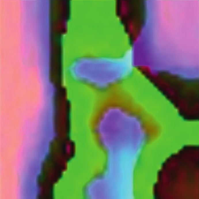
8 Computational Intelligence and Neuroscience

 Training/Testing (80:20) Accuracy Graph - (UCM21 Dataset)
 102
 1
 101 0.95
 100 0.9

 Accuracy Per Epoch
 99 0.85
 Values (%)

 0.8
 98
 0.75
 97
 0.7
 96 0.65

 95 0.6

 94 0 100 200 300 400 500 600
 Precision Recall Accuracy Epochs

 D-CNN VGG16-MSCP Training Accuracy
 SC-CNN LWCNN Model Validation Accuracy
 VGG-VD16-SAFF FCMBS-RSIC Figure 9: Accuracy analysis of FCMBS-RSIC technique on the
 Gated BD-GF UCM21 dataset.
Figure 7: Comparative analysis of the FCMBS-RSIC technique
under training/testing (80 : 20) data of the UCM21 dataset.
 Loss Graph - (UCM21 Dataset)
 Training/Testing (50:50)
 98
 0.6

 96 0.5
 Loss Per Epoch

 0.4
 94
 Values (%)

 0.3

 92 0.2

 0.1
 90
 0

 88 0 100 200 300 400 500 600
 Epochs
 Precision Recall Accuracy
 Training Loss
 D-CNN VGG16-MSCP
 Validation Loss
 SC-CNN LWCNN Model
 Figure 10: Loss analysis of FCMBS-RSIC technique on the UCM21
 VGG-VD16-SAFF FCMBS-RSIC dataset.
 Gated BD-GF
Figure 8: Comparative analysis of the FCMBS-RSIC technique
 A comprehensive classification result analysis of the
under training/testing (50 : 50) data of the UCM21 dataset.
 FCMBS-RSIC technique under varying sizes of training/
 testing data of UCM21 dataset is offered in Table 1.
simulated using Processor - i5-8600k, Graphics Card - Figure 7 examines the comparison study of the FCMBS-
GeForce 1050Ti 4 GB, 16 GB RAM, and OS Storage - 250 GB RSIC technique with recent methods [23] under training/
SSD. testing (80 : 20) data of UCM21 dataset. The experimental
 Figure 5 illustrates the preprocessed version of the test results revealed that the D-CNN, SC-CNN, and VGG-
RSI by the FCMBS-RSIC technique. The figures reported VD16-SAFF techniques have gained ineffective outcomes
that the image quality gets improved and it helps to increase with the least values of precn , recal , and accuy . Also, the
the classification outcomes of the FCMBS-RSIC technique. gated BD-GF and VGG16-MSCP techniques have attained
Figure 6 illustrates the feature maps obtained by the FCMBS- slightly raised values of precn , recal , and accuy . In addition,
RSIC technique on four test images namely airport, bare the LWCNN technique has gained somewhat reasonable
land, beach, and bridge. outcome with the precn , recal , and accuy of 97.76%, 99.55%,

Computational Intelligence and Neuroscience 9

 Table 2: Comparative analysis of the FCMBS-RSIC technique with existing approaches under the AID dataset.
 Training/testing (80 : 20) Training/testing (50 : 50)
Methods
 Precision Recall Accuracy Precision Recall Accuracy
D-CNN 89.81 91.10 90.82 95.78 97.77 96.89
SC-CNN 89.15 91.48 91.10 92.12 94.41 93.30
VGG-VD16-SAFF 89.18 90.49 90.25 92.51 95.46 93.83
Gated BD-GF 90.43 92.78 92.20 94.18 96.85 95.48
VGG16-MSCP 90.36 92.00 91.52 93.11 95.24 94.42
LWCNN model 92.51 94.18 93.85 96.22 98.75 97.64
FCMBS-RSIC 98.36 99.42 99.31 97.86 99.12 99.06

and 99.42%, respectively. However, the FCMBS-RSIC Training/Testing (80:20)
technique has shown better results with the precn , recal , and
 102
accuy of 98.12%, 99.67%, and 99.63%, respectively.
 Figure 8 illustrates the performance analysis of the 100
FCMBS-RSIC technique with existing techniques under
training/testing (50 : 50) data of the UCM21 dataset. The 98

 Values (%)
results indicated that the D-CNN, SC-CNN, and VGG-
 96
VD16-SAFF techniques have attained lower values of
precn , recal , and accuy . Concurrently, the gated BD-GF 94
and VGG16-MSCP techniques have resulted in somewhat
improved values of precn , recal , and accuy . Simultaneously, 92
the LWCNN technique has demonstrated considerable
 90
performance with the precn , recal , and accuy of 90.35%,
93.83%, and 92.10%. However, the FCMBS-RSIC tech- 88
nique has gained maximum performance with the precn , Precision Recall Accuracy
recal , and accuy of 94.12%, 95.32%, and 95.27%,
respectively. D-CNN VGG16-MSCP
 The accuracy outcome analysis of the FCMBS-RSIC SC-CNN LWCNN Model
technique on UCM21 dataset is portrayed in Figure 9. The VGG-VD16-SAFF FCMBS-RSIC
results demonstrated that the FCMBS-RSIC approach has
 Gated BD-GF
accomplished higher validation accuracy compared to
training accuracy. It is also observable that the accuracy Figure 11: Comparative analysis of the FCMBS-RSIC technique
values get saturated with the count of epoch. under training/testing (80 : 20) data of the AID dataset.
 The loss outcome analysis of the FCMBS-RSIC technique
on UCM21 dataset is illustrated in Figure 10. The figure
exposed that the FCMBS-RSIC system has denoted the training/testing (50 : 50) data of the AID dataset. The table
reduced validation loss over the training loss. It is addi- values revealed that the D-CNN, SC-CNN, and VGG-VD16-
tionally noticed that the loss values get saturated with the SAFF techniques have exhibited poor performance with the
count of epoch. minimum values of precn , recal , and accuy .
 Table 2 provides the RSI classification result analysis of Eventually, the gated BD-GF and VGG16-MSCP tech-
the FCMBS-RSIC technique under different sizes of train- niques have resulted in somewhat improved values of precn ,
ing/testing data of the AID dataset. recal , and accuy . Meanwhile, the LWCNN technique has
 Figure 11 inspects the classifier result analysis of the demonstrated considerable performance with the precn ,
FCMBS-RSIC technique with recent methods under train- recal , and accuy of 96.22%, 98.75%, and 97.64%. However,
ing/testing (80 : 20) data of AID dataset. The results indi- the FCMBS-RSIC technique has presented effective out-
cated that the D-CNN, SC-CNN, and VGG-VD16-SAFF comes with the precn , recal , and accuy of 97.86%, 99.12%,
techniques have accomplished worse outcomes with the and 99.06%, respectively.
lower values of precn , recal , and accuy . Besides, the gated The accuracy outcome analysis of the FCMBS-RSIC
BD-GF and VGG16-MSCP techniques have provided cer- method on AID dataset is showcased in Figure 13. The
tainly increased values of precn , recal , and accuy . The outcomes outperformed that the FCMBS-RSIC system has
LWCNN technique has exhibited competitive outcome with accomplished maximum validation accuracy compared to
the precn , recal , and accuy of 92.51%, 94.18%, and 93.85%. training accuracy. It is also observable that the accuracy
However, the FCMBS-RSIC technique has shown better values get saturated with the count of epoch.
results with the precn , recal , and accuy of 98.36%, 99.42%, The loss outcome analysis of the FCMBS-RSIC meth-
and 99.31%, respectively. odology on AID dataset is demonstrated in Figure 14. The
 Figure 12 reports the comparative result analysis of the figure is obvious that the FCMBS-RSIC technique has re-
FCMBS-RSIC technique with existing techniques under ferred to the lower validation loss over the training loss. It

10 Computational Intelligence and Neuroscience

 Training/Testing (50:50) Loss Graph - (AID Dataset)
 0.7
 102
 0.6
 100
 0.5

 Loss Per Epoch
 98
 0.4
 Values (%)

 96
 0.3
 94
 0.2
 92 0.1
 90 0

 88 0 100 200 300 400 500 600 700 800
 Precision Recall Accuracy Epochs

 D-CNN VGG16-MSCP Training Loss
 SC-CNN LWCNN Model Validation Loss
 VGG-VD16-SAFF FCMBS-RSIC Figure 14: Loss analysis of FCMBS-RSIC technique on the AID
 Gated BD-GF dataset.
Figure 12: Comparative analysis of the FCMBS-RSIC technique
under training/testing (80 : 20) data of AID dataset.
 Table 3: Computation time analysis of FCMBS-RSIC technique
 under two datasets.
 Accuracy Graph - (AID Dataset) Computation time (sec)
 1 Methods UCM21 dataset AID dataset
 D-CNN 354 383
 0.9 SC-CNN 136 198
 Accuracy Per Epoch

 VGG-VD16-SAFF 116 125
 0.8 Gated BD-GF 262 332
 VGG16-MSCP 181 272
 0.7 LWCNN model 089 074
 FCMBS-RSIC 064 058
 0.6

 0.5
 0 100 200 300 400 500 600 700 800 450

 Epochs 400
 Computation Time (sec)

 350
 Training Accuracy 300
 Validation Accuracy 250
Figure 13: Accuracy analysis of the FCMBS-RSIC technique on 200
AID dataset. 150
 100
 50
can be additionally noticed that the loss values get saturated
 D-CNN

 SC-CNN

 VGG-VD16-SAFF

 Gated BD-GF

 VGG16-MSCP

 LWCNN Model

 FCMBS-RSIC

with the count of epoch.
 Lastly, a detailed computation time (CT) analysis of the
FCMBS-RSIC technique on the test UCM21 and AID datasets
is given in Table 3 and Figure 15. The experimental values
indicated that the D-CNN model has shown ineffective results
with the maximum CT on the test datasets. In addition, the
 UCM21 Dataset
gated BD-GF and VGG16-MSCP techniques have resulted in
slightly reduced CT over the D-CNN technique. AID Dataset
 Along with that, the SC-CNN and VGG-VD16-SAFF Figure 15: CT analysis of FCMBS-RSIC technique with existing
techniques have reached moderately closer CT. Though the methods.

Computational Intelligence and Neuroscience 11

LWCNN technique has attained reasonable CT of 89s and classification,” Pattern Recognition Letters, vol. 140, pp. 186–
74s on the UCM21 and AID datasets, the proposed FCMBS- 192, 2020.
RSIC technique has outperformed the other methods with [2] A. Joshi, A. Dhumka, Y. Dhiman, C. Rawat, and fnm Ritika,
the lower CT of 64s and 58s, respectively. By looking into the “A comparative study of supervised learning techniques for
above mentioned tables and figures, it is ensured that the remote sensing image classification,” in Advances in Intelli-
 gent Systems and Computing Soft Computing: Theories and
FCMBS-RSIC technique has the ability of effectually classify
 ApplicationsSpringer, Singapore, 2022.
RSIs. [3] W. Sun, K. Ren, X. Meng, C. Xiao, G. Yang, and J. Peng, “A
 band divide-and-conquer multispectral and hyperspectral
5. Conclusion image fusion method,” IEEE Transactions on Geoscience and
 Remote Sensing, vol. 60, Article ID 5502113, 2021.
In this study, a new FCMBS-RSIC methodology was de- [4] F. Xie, M. Shi, Z. Shi, J. Yin, and D. Zhao, “Multilevel cloud
veloped for the detection and classification of RSIs. The detection in remote sensing images based on deep learning,”
proposed FCMBS-RSIC method encompasses different Ieee Journal of Selected Topics in Applied Earth Observations
subprocesses such as preprocessing, RetinaNet-based feature and Remote Sensing, vol. 10, no. 8, pp. 3631–3640, 2017.
extraction, FCM-based classification, and BSA-based pa- [5] G. J. Scott, M. R. England, W. A. Starms, R. A. Marcum, and
rameter tuning. The design of BSA helps to properly tune the C. H. Davis, “Training deep convolutional neural networks for
 land-cover classification of high-resolution imagery,” IEEE
parameters contained in the FCM model, and consequently,
 Geoscience and Remote Sensing Letters, vol. 14, no. 4,
the classification efficiency can be improved. The perfor- pp. 549–553, 2017.
mance validation of the FCMBS-RSIC technique takes place [6] C. Peng, Y. Li, L. Jiao, and R. Shang, “Efficient convolutional
using benchmark open access datasets and the results are neural architecture search for remote sensing image scene
examined under several aspects. The comparative experi- classification,” IEEE Transactions on Geoscience and Remote
mental outcomes described the enhanced outcomes of the Sensing, vol. 59, no. 7, pp. 6092–6105, 2021.
FCMBS-RSIC method over its recent approaches. Therefore, [7] H. Li, Z. Cui, Z. Zhu et al., “RS-MetaNet: deep metametric
the FCMBS-RSIC technique can be treated as an effective learning for few-shot remote sensing scene classification,”
tool for RSI classification. In future, hybrid DL models can IEEE Transactions on Geoscience and Remote Sensing, vol. 59,
be derived to improve the classifier results of the FCMBS- pp. 1–12, 2020.
 [8] H. Chen and Z. Shi, “A spatial-temporal attention-based
RSIC technique.
 method and a new dataset for remote sensing image change
 detection,” Remote Sensing, vol. 12, no. 10, p. 1662, 2020.
Data Availability [9] A. M. Hilal, F. N. Al-Wesabi, K. J. Alzahrani et al., “Deep
 transfer learning based fusion model for environmental re-
Data sharing is not applicable to this article as no datasets mote sensing image classification model,” European Journal of
were generated during this study. Remote Sensing, pp. 1–12, 2022.
 [10] W. Zhang, P. Tang, and L. Zhao, “Remote sensing image scene
Conflicts of Interest classification using CNN-CapsNet,” Remote Sensing, vol. 11,
 no. 5, p. 494, 2019.
The authors declare that they have no conflicts of interest. [11] O. A. Shawky, A. Hagag, E.-S. A. El-Dahshan, and
 M. A. Ismail, “Remote sensing image scene classification using
 CNN-MLP with data augmentation,” Optik, vol. 221, Article
Authors’ Contributions ID 165356, 2020.
 [12] Y. Li, Y. Zhang, and Z. Zhu, “Error-tolerant deep learning for
The manuscript was written through contributions of all remote sensing image scene classification,” IEEE Transactions
authors. All authors have given approval to the final version on Cybernetics, vol. 51, no. 4, pp. 1756–1768, 2020.
of the manuscript. [13] X. Xu, Y. Chen, J. Zhang, Y. Chen, P. Anandhan, and
 A. Manickam, “A novel approach for scene classification from
Acknowledgments remote sensing images using deep learning methods,” Eu-
 ropean Journal of Remote Sensing, vol. 54, no. 2, pp. 383–395,
The authors extend their appreciation to the Deanship of 2021.
Scientific Research at King Khalid University for funding [14] L. Min, K. Gao, H. Wang et al., “Remote sensing image scene
this work under grant number RGP2/18/43 and Princess classification using deep combinative feature learning,” in
Nourah Bint Abdulrahman University Researchers Sup- Proceedings of the AOPC 2020: Optical Sensing and Imaging
porting Project (PNURSP2022R303), Princess Nourah Bint Technology, vol. 11567, November 2020, Article ID 115672N.
 [15] W. Huang, Z. Yuan, A. Yang, C. Tang, and X. Luo, “TAE-net:
Abdulrahman University, Riyadh, Saudi Arabia. The authors
 task-adaptive embedding network for few-shot remote
would like to thank the Deanship of Scientific Research at sensing scene classification,” Remote Sensing, vol. 14, no. 1,
Umm Al-Qura University for supporting this work by Grant p. 111, 2022.
Code: 22UQU4310373DSR05. [16] L. Yin, P. Yang, K. Mao, and Q. Liu, “Remote sensing image
 scene classification based on fusion method,” Journal of
References Sensors, vol. 2021, Article ID 6659831, 14 pages, 2021.
 [17] P. Yun, L. Tai, Y. Wang, C. Liu, and M. Liu, “Focal loss in 3d
 [1] W. Jing, Q. Ren, J. Zhou, and H. Song, “AutoRSISC: automatic object detection,” IEEE Robotics and Automation Letters,
 design of neural architecture for remote sensing image scene vol. 4, 2019.

12 Computational Intelligence and Neuroscience

[18] C. D. Stylios, V. C. Georgopoulos, G. A. Malandraki, and
 S. Chouliara, “Fuzzy cognitive map architectures for medical
 decision support systems,” Applied Soft Computing, vol. 8,
 no. 3, pp. 1243–1251, 2008.
[19] X.-B. Meng, X. Z. Gao, L. Lu, Y. Liu, and H. Zhang, “A new
 bio-inspired optimisation algorithm: bird Swarm Algorithm,”
 Journal of Experimental & Theoretical Artificial Intelligence,
 vol. 28, no. 4, pp. 673–687, 2016.
[20] J. Zhang, K. Xia, Z. He, and S. Fan, “Dynamic Multi-Swarm
 Differential Learning Quantum Bird Swarm Algorithm and its
 Application in Random Forest Classification Model,” Com-
 putational Intelligence and Neuroscience, vol. 2020, Article ID
 6858541, 24 pages, 2020.
[21] Y. Yang and S. Newsam, “Bag-Of-Visual-Words and Spatial
 Extensions for Land-Use Classification,” in Proceedings of the
 ACM SIGSPATIAL International Conference on Advances in
 Geographic Information Systems (ACM GIS), New York, NY,
 USA, November 2010.
[22] X. Gui-Song, H. Jingwen, H. Fan et al., “AID: A Benchmark
 Dataset for Performance Evaluation of Aerial Scene Classi-
 fication,” IEEE Trans. on Geoscience and Remote Sensing,
 vol. 7, 2016.
[23] C. Shi, X. Zhang, J. Sun, and L. Wang, “A lightweight con-
 volutional neural network based on group-wise hybrid at-
 tention for remote sensing scene classification,” Remote
 Sensing, vol. 14, no. 1, p. 161, 2022.