From Phase Transition to Interdecadal Changes of ENSO, Altered by the Lower Stratospheric Ozone
←
→
Page content transcription
If your browser does not render page correctly, please read the page content below
remote sensing
Communication
From Phase Transition to Interdecadal Changes of ENSO,
Altered by the Lower Stratospheric Ozone
Natalya Andreeva Kilifarska *, Tsvetelina Plamenova Velichkova and Ekaterina Anguelova Batchvarova

                                          Climate, Atmosphere and Water Research Institute, Bulgarian Academy of Sciences, 66, Tsarigradsko Shosse Blvd,
                                          1784 Sofia, Bulgaria; tsvetelinavelichkova@cawri.bas.bg (T.P.V.); ekbatch@cawri.bas.bg (E.A.B.)
                                          * Correspondence: nkilifarska@cawri.bas.bg or natalya_kilifarska@yahoo.co.uk

                                          Abstract: This paper shows more evidence for the existing spatial–temporal synchronization of the air
                                          surface temperature and pressure within the lower stratospheric ozone, which is unevenly distributed
                                          over the globe. The focus of this study is put on the region of formation and manifestation of El Niño
                                          Southern Oscillation (ENSO). Statistical analysis of data (covering the period 1900–2019) displays
                                          a well pronounced covariance of ozone at 70 hPa with (i) Nino3.4 index, (ii) air surface temperature,
                                          and (iii) sea level pressure, in each grid-point with spatial resolution of 5◦ in latitude and longitude.
                                          The ozone impact could be found at different time scales—from interannual (altering the ENSO phase
                                          transition) to interdecadal. Moreover, the centers of action of ozone on the sea level temperature
                                          and pressure are positioned at different places, depending on the temporal scale of variability—from
                                          the tropical Central Pacific—at interannual and interdecadal, to extratropics—at subdecadal time
                                          scales. We show also that positive ozone anomalies at 70 hPa trigger a cooling of the sea surface, with
                                          a delay of 9 record’s time intervals. The ozone depletion, on the other side, is followed by a sea level
                                          warming with a delay of 1–2 record’s time intervals.

                                Keywords: El Niño; La Niña; ENSO; lower stratospheric ozone

Citation: Kilifarska, N.A.;
Velichkova, T.P.; Batchvarova, E.A.
From Phase Transition to
Interdecadal Changes of ENSO,
                                          1. Introduction
Altered by the Lower Stratospheric              The El Niño Southern Oscillation (ENSO) manifests itself as recurring changes of
Ozone. Remote Sens. 2022, 14, 1429.       the sea surface temperature and sea level pressure over the tropical Pacific Ocean. ENSO
https://doi.org/10.3390/rs14061429        fluctuates between its main phases—La Niña and El Niño—with a periodicity of 2–7 years.
Academic Editor: Beatriz M. Funatsu
                                          Despite the uniformity of solar radiation, received by the tropical region, the sea surface
                                          temperature there is asymmetrically distributed in space. Thus, during the La Niña phase,
Received: 31 January 2022                 the eastern tropical Pacific (i.e., the coasts of Ecuador and Peru) is cooler, while the western
Accepted: 11 March 2022                   one (i.e., the coastal regions of Indonesia and Australia) is warmer. This asymmetry is,
Published: 15 March 2022                  however, reversed periodically and then the eastern tropical Pacific becomes warmer than
Publisher’s Note: MDPI stays neutral      usual (El Niño phase).
with regard to jurisdictional claims in         Besides this classical manifestation of ENSO, another type of El Niño warming has
published maps and institutional affil-   been discovered, which is located in the central, instead of the eastern, Pacific Ocean [1–3].
iations.                                  In the scientific literature this type of El Niño is referred to as dateline El Niño, El Niño
                                          Modoki, Warm Pool El Niño or Central Pacific (CP) El Niño. The observational data and
                                          models’ simulations indicate an increased probability of appearance of the CP El Niño,
                                          after 1990—possibly related to anthropogenic climate change [4].
Copyright: © 2022 by the authors.               The consecutive alternation of cold and warm ENSO phases is recently explained
Licensee MDPI, Basel, Switzerland.
                                          in light of a signal processing theory. Both competing explanations differ by the strength
This article is an open access article
                                          of coupling of the atmosphere–ocean system. Thus, the nonlinear hypothesis implies that
distributed under the terms and
                                          the oceanic feedback (to the atmospheric forcing) is strong enough to maintain the self–
conditions of the Creative Commons
                                          sustained oscillation between a cold and a warm phase. In addition, the coupled ocean–
Attribution (CC BY) license (https://
                                          atmosphere system interacts nonlinearly with the annual cycle of the sea surface temper-
creativecommons.org/licenses/by/
4.0/).
                                          ature (driven by the received solar radiation). This interaction ensures the irregularity

Remote Sens. 2022, 14, 1429. https://doi.org/10.3390/rs14061429                                        https://www.mdpi.com/journal/remotesensing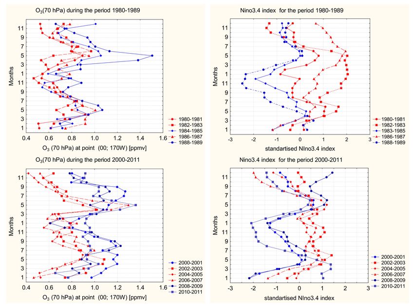
Remote Sens. 2022, 14, 1429                                                                                           2 of 15

                              of consecutive ENSO phases (due to the different frequencies of driving annual cycle
                              and oscillating frequency of the coupled system). According to the stochastic hypothesis
                              the atmosphere–ocean system is coupled in a weak feedback regime, which does not sup-
                              port a self–sustained oscillation. The transition between ENSO phases in this framework is
                              attributed to the ‘weather noise’ generated by the hydrodynamic instability of the atmo-
                              sphere [5]. Examples of such initial forcing for the coupled system could be westerly wind
                              bursts, tropical instability waves, monsoon activity, Madden-Julian oscillation, extratropical
                              forcing, etc. [6]. The irregularity of the ENSO cycle in this case is ensured by the random
                              initial forcing.
                                    According to our point of view, these explanations of ENSO dynamics are rather ‘tech-
                              nical’ and do not provide a physically sound explanation of irregularly changing (in space
                              and time) regimes of the sea–surface temperature in the tropical Pacific Ocean. One recent
                              attempt for more physical explanation is offered by Lin and Qian [7], demonstrating that
                              the switch between El Niño and La Niña is caused by a subsurface ocean wave, propagat-
                              ing from the western to the central and eastern parts of the Pacific Ocean. The potential
                              driver of such decoupled from the atmosphere, subsurface oceanic wave, the authors see
                              in the lunar tidal gravitational force, and more specifically in the interaction between its
                              6th and 9th year frequency peaks [7].
                                    On the other hand, the lower stratospheric ozone influence on the Walker circulation [8]
                              and the near surface temperature [9], as well as a detected relation between interdecadal
                              variability of Nino3.4 index and lower stratospheric ozone [10], motivated us to study
                              the possibility for ozone influence on ENSO variability on different time scales. The spatial–
                              temporal irregularity of the lower stratospheric ozone—related to the solar and geomagnetic
                              modulation of cosmic radiation reaching the lower stratospheric levels [9]—could be
                              a reasonable explanation of the irregular behavior of the ENSO climatic mode.

                              2. Data and Methods
                                    Data for air temperature at 2 m above the surface, sea level atmospheric pressure and
                              ozone at 70 hPa have been taken from two reanalyzes: ERA 20 Century (https://apps.
                              ecmwf.int/datasets/data/era20cm-edmm/levtype=sfc, accessed on 11 November 2015)
                              and ERA-Interim (https://apps.ecmwf.int/datasets/data/interim-full-daily/levtype=sfc,
                              10 March 2021). The length of ERA 20C has been extended by data from ERA Interim after
                              2010, in order to include the recent period, characterized by a different manifestation of
                              the El Niño phase. Both reanalyzes were merged at the year 2000. The merging procedure
                              includes an equalization of the decadal means of both reanalyzes, for the period 2001–2010.
                              This procedure ensures a smooth transition between the two reanalyzes, avoiding the step-
                              like changes between their means. Monthly records of all atmospheric variables have been
                              derived in a grid with 5 deg step in latitude and longitude. In addition, monthly values
                              of the ozone profile, provided from the ERA Interim for the period 1979–2019, have been
                              derived at all meteorological levels up to 10 hPa.
                                    The interdecadal and interannual variability of atmospheric variables has been investi-
                              gated by the use of their winter values (calculated over the December-April months)—i.e.,
                              the data records contain one value per year. The transition between different ENSO phases,
                              however, has been investigated by the use of monthly data, in order to ensure a statistical
                              significance of the results. Moreover, for a reduction of the within-group variation, two
                              subsamples have been created, corresponding to the El Niño and La Niña phase. Due to
                              the fact that both ENSO phases are better pronounced in the winter season, the El Niño
                              and La Niña composites have been created from the monthly values within the period
                              November-April. The discrimination between positive and negative ENSO phases has been
                              done by the use of Nino3.4 index, imposing the following criteria: all months with Nino3.4
                              greater than records’ mean + 1 standard deviation are added to the El Niño sample, while
                              months for which Nino3.4 index is less that the index’s record mean, reduced by 1 standard
                              deviation, are selected for the La Niña sample. The data in these composites retain the time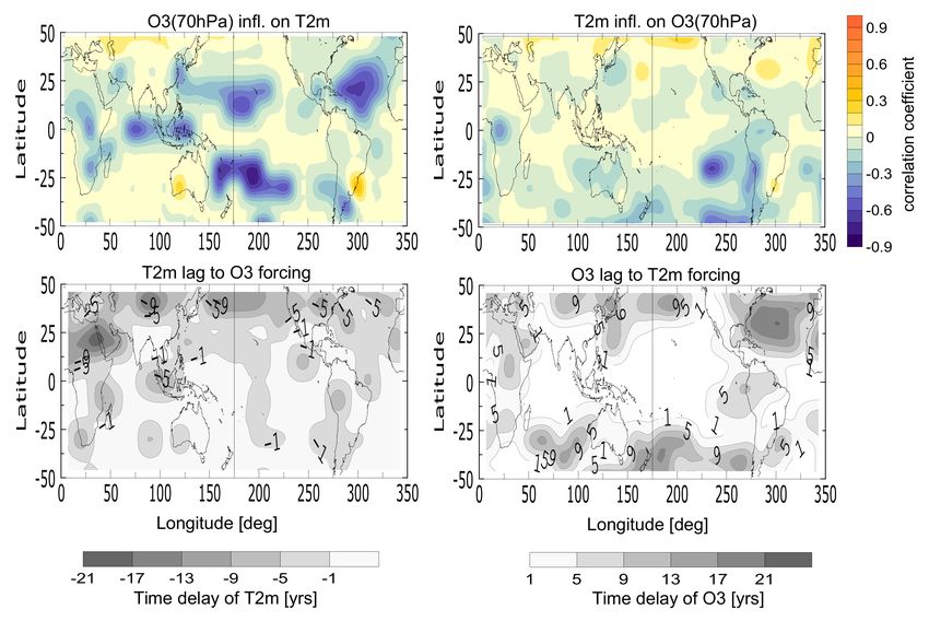
Remote Sens. 2022, 14, 1429                                                                                              3 of 15

                              sequence but are unevenly distributed along the time axis. For this reason, the analysis of
                              the lagged response of their variables is reported in the irregular record’s time intervals.
                                   The possible relationship between lower stratospheric ozone and climatic variables
                              has been sought on different time scales. For this reason, the time series of all variables
                              have been smoothed by running averaging procedure over 3, 5 or 11 points, depending
                              on the specific purpose. Thus, the existence of relations at interdecadal time scales has
                              been estimated from mean winter values, smoothed by 11-year running window. Similarly,
                              the variability at the subdecadal time scale has been studied from the seasonal (winter)
                              records, smoothed by 5-year running average procedure. The interannual variability
                              of ENSO phases, however, has been performed by the use of monthly values and data
                              have been smoothed by a 3-point moving window in order to filter the highest frequency
                              variations. Data smoothing allows the discovery of long-term variations, which otherwise
                              are masked by the short-term fluctuations of examined variables.
                                   Dynamical anomalies (dO3 ) of ozone density has been used as another measure of its
                              temporal variations. They have been calculated as the difference between a dynamically
                              evolving decadal mean for a given moment, and the measured value at that moment,
                              in each point of our data grid (Equation (1)):

                                            dO3 (t, lat, long, lev) = O3 (t, lat, long, lev) − O3 (t, lat, long, lev)       (1)

                              where the dO3 (t, lat, long, lev) is the record’s mean value (corresponding to the moment t),
                              which is a non-linear function of time, on decadal time scales. The calculation of dynamical
                              anomalies is equivalent to a non-linear de-trending of data records.
                                   The temporal covariance between lower stratospheric ozone, near surface temperature
                              (T2m ) and sea level pressure is estimated by the use of the lagged cross-correlation, known
                              also as a distributed lags analysis. Due to the fact that the cross-correlation function is not
                              symmetrical about the zero lag, in the STATISTICA package the independent (i.e., first,
                              or leading) variable is moved first backward, and then forward. The cross-correlation
                              coefficient with lag k is computed following the standard formulas, as described in most
                              time series references (e.g., [11]):

                                               rxy (k) = cxy (k)/ sx sy , for k = 0, ±1, ±2, ±3, . . . . . . . . . .

                              where cxy is the cross-covariance coefficients at lag k, sx and sy are standard deviations of
                              series X and Y respectively, calculated as usual by the formulas:
                                                               s                            s
                                                                              2                           2
                                                                   ∑ Xt − X                     ∑ Yt − Y
                                                        sx =                       ; sy =
                                                                       N                            N

                              where N is the number of the observations in time series and X and Y are records’ mean
                              values. The cross covariance function is calculated as follow:
                                                  1    N
                                                    · ∑t=1−k Yt − Y · Xt+k − X for k = −1, −2, . . . − (N − 1)

                                      cxy (k) =                                                                             (2)
                                                  N
                                                   1     N−k
                                                     · ∑t=1 Yt − Y · Xt+k − X for k = 0, 1, 2, . . . N − 1

                                         cxy (k) =                                                                          (3)
                                                   N
                                   Equation (2) describes the delayed response of Y to changes of X in moment t, and its
                              time lag is given by a negative number. Equation (3) describes the lagged response of X
                              to the changes of Y in the moment t. For this reason, the time delay in the maps of lagged
                              response could be a positive or negative number.
                                   Correlation maps, illustrating the spatial irregularities in the strength of the covariance
                              between analyzed variables, have been created from the statistically significant at 2σ level
                              correlation coefficients. The time delay of the response variable has been determined
                              by choosing the maximal cross-correlation coefficient, among all statistically significant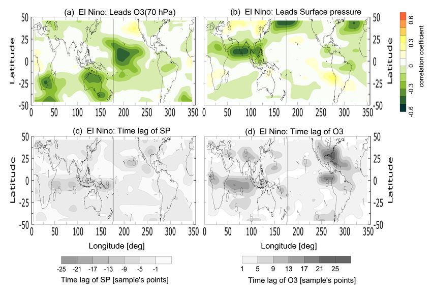
Remote Sens. 2022, 14, 1429                                                                                                  4 of 15

                                  coefficients, calculated with time lags from 0 to 25 (at interdecadal time scales—with
                                  maximal lag of 35 years).
                                         Estimation of the confidence of the calculated correlations is an indispensable part of
                                  the analysis. However, the standard test of significance of correlations between serially
                                  correlated records (i.e., with nonzero autocorrelation) could inflate the calculated Z-values,
                                  producing false positives when testing the validity of the null hypothesis H0 , assuming
                                  that both time series do not correlate, i.e., rXY = 0. To solve this problem, we have used
                                  the methodology proposed by [12] consisting of the determination of two factors: (i) re-
                                  calculation of the variance of the correlation coefficients, taking into account not only
                                  the autocorrelation coefficients of both time series, but also their cross-correlation and
                                  (ii) the effective degree of freedom, being reduced in serially correlated records.
                                         In a case of stationary covariance, the authors of [12] proposed the following formula
                                  for the calculation of samples’ correlation coefficients’ variance:

                                                            2      M
                                   −2
                   var(rXY,k ) = N         (N − 2)· 1 − r20 + r20 · ∑ (N − 2 − k)· r2XX,k + r2YY,k + r2XY,k ·r2YX,−k
                                                                 k=1
                                             M
                                       −2r0 ∑ (N − 2 − k)·(rXX,k + rYY,k )·(rXY,k + rYX,−k )                                    (4)
                                           k=1
                                           M
                                       +2 ∑ (N − 2 − k)·(rXX,k ·rYY,k + rXY,k ·rYX,−k )
                                           k=1

                                  where r0 is the zero lag cross-correlation coefficient between variables X and Y; rXX,k and
                                  rYY,k are their autocorrelation coefficients with lag k; M is the truncation of autocorrelation
                                  functions (ACF), above which the ACF is assumed to become zero. Various authors have
                                  used different suggestions for the choice of M (e.g., [12–14]). We adopted the value N        4
                                  as has been proposed by Anderson. The refined rXY,k variance has been used then to
                                  calculate the variance of its transformed value by the Fisher’s Z-transformation, defined as
                                  FXY,k = arctangh(rXY,k ), i.e.,
                                                                                                  −2
                                                               var(FXY,k ) = var(rXY,k )· 1 − r20                               (5)

                                       Finally, the Z-value, used to detect statistical confidence of the result has been calcu-
                                  lated by the formula [12]:

                                                                       FXY               arctanh(rXY )
                                                         ZXY = p                = q                          −2                (6)
                                                                    var(FXY )         var(rXY )· 1 − r2XY

                                       The second method applied to assess the possible inflation of correlation coefficients,
                                  due to the autocorrelation of examined time series, is through the determination of effective
                                  degrees of freedom (EDF). There are several formulas suggested in the scientific literature,
                                  but all of them rely on the assumption for uncorrelated (but auto-correlated) records.
                                  This requirement is not met by our time series, because they covariate in time and our
                                  main purpose is to estimate the strength and reliability of their correlation. Nevertheless,
                                  we made this assessment using the formula presented in the work of [12]:
                                                                                                           ! −1
                                                                             N−1
                                                                                   (N − k)
                                                          Neff = N 1 + 2     ∑       N
                                                                                           ·rXX,k ·rYY,k                        (7)
                                                                             k=1

                                       The results of this analysis are discussed in the “Results” section with a pre-defiled
                                  level of confidence α = 0.05.
                                       Besides the statistical significance of calculated correlations, there is another difficulty,
                                  related to the spatial distribution of variables’ temporal covariation. More specifically,
                                  the calculated lagged correlation coefficients have different time lags in different points
                                  of our grid, which makes it difficult to compare them directly. For this reason, they have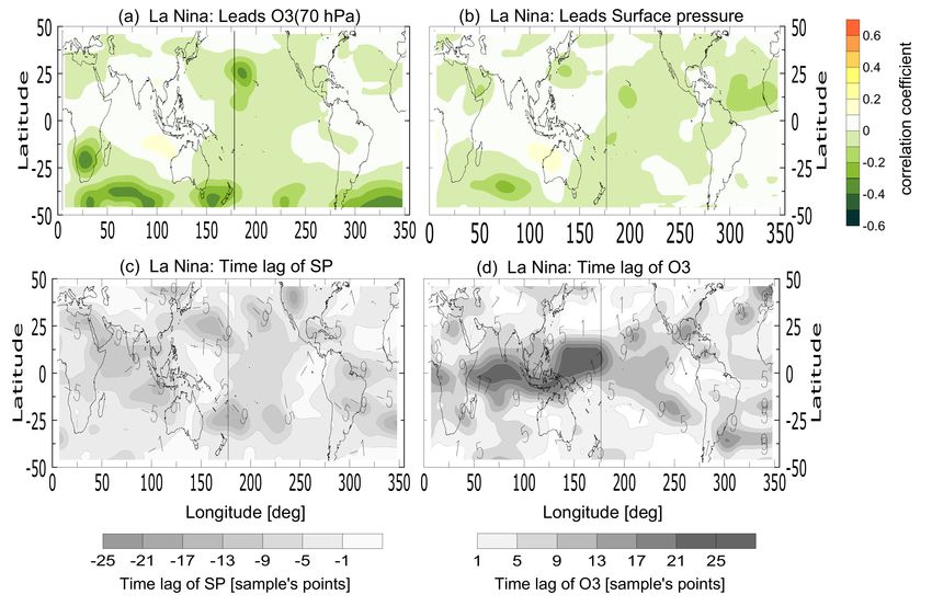
Remote Sens. 2022, 14, 1429                                                                                                   5 of 15

                              been preliminarily weighted by the autocorrelation function of the impact factor—with
                              a lag corresponding to the delay of the response variable to the applied forcing. Although
                              this procedure reduces the strength of the relation, it allows us to compare the correlation
                              coefficients with different time lags (for more details see chapter 12 in [15]). The reasoning
                              for such a weighting is based on the assumption that the effect of the applied (in a given
                              moment in time) forcing decreases with moving away from this moment.

                              3. Results
                              3.1. Interdecadal and Subdecadal Variability of the Lower Stratospheric Ozone and Surface
                              Temperature
                                   Previous analysis of the centennial variability of lower stratospheric ozone and Nino3.4
                              index [10] reveals the existence of a strong, well-pronounced covariance over the central
                              Pacific Ocean and Maritime continent (see Figure 1). The one winter season time delay of
                              the Nino3.4 response (following the variations of the lower stratospheric ozone) is quite
                              promising for a possible ozone modulation of the central Pacific near-surface temperature
                              (the mechanism of influence is described in [10]).

                              Figure 1. (a) Cross-correlation maps of the lower stratospheric ozone (the leading factor) and Nino3.4
                              index calculated from the winter values (December–April), over the period 1900–2010 (colored
                              shading). (b) Time delay of Nino3.4 response to the chances of ozone density at 70 hPa (adapted from
                              Velichkova and Kilifarska [10], their Figure 3).

                                    Due to the fact that we are working with smoothed time records, the autocorrelation
                              of which reduces the available degrees of freedom, the confidence of the inferred ozone
                              influence on the Nino3.4 index is tested using two statistical tests (i.e., the Z-test and
                              the t-test, as described in “Data and Methods” section). Results from the tests are presented
                              in Table 1 (the 1st row). The p-value is derived after the Fisher’s transformation of the max-
                              imal cross-correlation coefficient (calculated in the point with coordinates: 10◦ N; 190◦ E)
                              and correction of its variance for autocorrelation and cross-correlation of both variables
                              (Equation (4)). The Z-value, calculated by Equation (5), is then used to find the correspond-
                              ing p-value. Note that the derived p-value (in the region of strongest coupling between O3
                              and NAO) is much less than the initially chosen level of significance α = 0.05. Thus, the 1st
                              test rejects the null hypothesis (suggesting that rXY,k = 0).
                                    The second test, based on the assessment of the effective degrees of freedom (EDF),
                              gives worse results, but anyhow, the calculated correlation coefficient is still higher than
                              the critical value of rXY = 0.5. Consequently, the hypothesis testing passes both tests of
                              significance and we could conclude that at a confidence level of 5%, the correlation between
                              O3 at 70 hPa and Nino3.4 index is not the result of chance.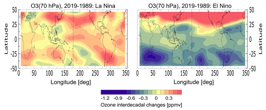
Remote Sens. 2022, 14, 1429                                                                                                          6 of 15

                                       Table 1. Values of maximal lagged correlation coefficients at some regions with well-defined covari-
                                       ance between studied variables, their p-values and critical correlations, calculated by two methods
                                       (Z-test and t-test) after accounting for the autocorrelation of analyzed time records.

                                             Corrected Variance of rxy → Z test                           Students’ t-Test
   Correlated Variables                        Time Lag of         Corrected                N–Number                Critical
                                  Max. rxy                                        p-Value                EDF                   Critical rxy
                                              Response Var.         Z-Score                 of Observ.            t = f(EDF)
         O3 & NAO                 −0.663            −3               −6.18           0         101        14         2.15         0.50
  O3 & T2m (20◦ N;190◦ E)         −0.648            −1               −6.56           0         107        16         2.12         0.46
  O3 & T2m   (30◦   S;190◦   E)    −0.70            −2               −3.38        0.0008       107        11          2.2         0.56
    EN: O3 & Surf.Press.
                                   −0.68            −1               −8.15           0         123        43         2.017        0.29
      (10◦ N;190◦ E)
    LN: O3 & Surf.Press.
                                   −0.43            −1               −3.38         0.008       139        45         2.013        0.28
      (25◦ N;190◦ E)

                                             The covariance between ozone and Nin3.4 index has been calculated from time records
                                       smoothed by an 11-year moving window, and the obtained relation is valid on interdecadal
                                       time scales. The Nino3.4 index, however, reflects the specific temperature variability over
                                       the central Pacific, while the ozone influence on the surface temperature is most probably
                                       local. Consequently, the detection of the ozone–temperature connection is possible only
                                                                                                                         ◦
                                       through their comparison in each point of the data grid (in our case with 5 increments
                                       in latitude and longitude). Moreover, due to the fact that the mean period of ENSO
                                       variability is about 5 years, we have smoothed the ozone and temperature data by a 5-point
                                       moving window.
                                             Two hypotheses have been estimated: (i) near-surface temperature (T2m ) influences
                                       ozone at 70 hPa (via tropical convection and cross-tropopause isentropic mixing with
                                       extratropics [16]), and (ii) ozone affects the T2m through modulation of the upper tropo-
                                       sphere static stability, followed by a moistening or drying of the upper troposphere and
                                       alteration of the strength of the greenhouse effect [17]. The ozone–temperature correlation
                                       maps (shown in Figure 2) have been created by cross-correlation coefficients, preliminarily
                                       weighted by the autocorrelation function of the forcing factor, with a lag corresponding to
                                       the time lag of the dependent variable.
                                             A glance at Figure 2 reveals two main findings: (i) the temporal covariance between
                                       ozone and temperature is irregularly distributed over the globe; (ii) the ozone’s influence
                                       on the temperature is stronger, especially near the dateline in both subtropics, as well as over
                                       the Maritime continent and the South Atlantic Ocean. The time delay of T2m response is 1–2
                                       winter seasons (see the bottom panel in Figure 2). Figure 2 suggests also that the irregularity
                                       of the ENSO cycle could be influenced by the variability of the lower stratospheric ozone
                                       density through the influence on the off-equatorial sea surface temperature anomalies [18].
                                       The statistical significance of this result has been estimated in two regions, for which
                                       the strongest covariance between both variables has been found (more specifically at points
                                       with coordinates 20◦ N; 190◦ E and 30◦ S; 190◦ E). Too methods have been used, accounting
                                       for autocorrelation and cross-correlation of both records. The results are shown in the 2nd
                                       and 3rd rows of Table 1. Note that the strength of the correlation between ozone and T2m
                                       passes both tests of significance.
                                             This result reasonably raises a question about the driver(s) of ozone variability itself.
                                       Although there are many factors influencing the lower stratospheric ozone, what is impor-
                                       tant for us are those factors outside the climatic system, because otherwise we will not be
                                       able to establish the causality. An exhaustive explanation of the external factors influencing
                                       the lower stratospheric ozone could be found in [9].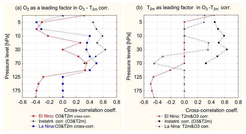
Remote Sens. 2022, 14, 1429                                                                                                 7 of 15

                              Figure 2. Correlation maps of the lower stratospheric ozone mixing ratio and temperature at 2 m
                              above the surface (T2m ), calculated for December–April during the period 1900–2010. The colored
                              shading marks the lagged cross-correlation. The upper left panel illustrates the hypothesis for O3 as
                              an independent variable, while the upper right panel shows the strength of T2m influence on the O3 .
                              The bottom panels show the spatial distribution of the time lag of dependent variables in years.

                              3.2. ENSO Cycle and Temporal–Spatial Variability of the Lower Stratospheric Ozone
                                    The transition between cold and warm ENSO phases is traditionally attributed to the cou-
                              pling between atmosphere and ocean—two systems with different heat capacities, different
                              heat conductivity, inertia, etc. One weakness of existing hypotheses, however, is the unverifi-
                              able assumption about the strength of oceanic feedback—ensuring or not the self-sustained
                              oscillation of the coupled atmosphere–ocean system. In addition, the missing physical rea-
                              soning about the burst of the initial ENSO forcing (required by the stochastic hypothesis) is
                              another deficiency of existing theories about ENSO variability. Moreover, the discovery of dif-
                              ferent types of El Niño raises the necessity of a better physical understanding of the processes
                              affecting the tropical sea surface temperature and pressure variability.
                                    This section is focused on the interannual variability of the sea level pressure and
                              its relation to the lower stratospheric ozone density. Some authors have investigated
                              the imprint of the warm El Niño phase on the stratospheric ozone [19–21], which is missing
                              during the cold La Niña phase. For this reason, we have created two composites of monthly
                              ozone and sea level pressure records, corresponding to both ENSO phases. In order to
                              increase the number of analyzed cold and warm events, we have used the merged ERA
                              20C and ERA Interim reanalyzes, covering the period 1900–2019, from November to April
                              each year. The monthly data have been smoothed by a 3-points running average procedure.
                              Unlike the previous investigations, examining dynamical influence of the tropospheric
                              convection and the Brewer–Dobson circulation on the lower stratospheric ozone, we have
                              analyzed the two possibilities: (i) the sea level pressure effect on the ozone and (ii) the lower
                              stratospheric ozone influence on the near surface temperature and pressure. The problem of
                              causality has been resolved by the use of the lagged cross-correlation analysis. The lagged
                              correlation coefficients, used for the creation of correlation maps shown in Figures 3 and 4,
                              have been initially weighted by the autocorrelation function of the forcing variable, allowing
                              us to compare the strength of correlation with different time lags.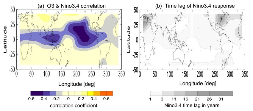
Remote Sens. 2022, 14, 1429                                                                                                 8 of 15

                              Figure 3. Maps of lagged cross-correlation between the ozone at 70 hPa and sea level pressure
                              (coloured shading in top panels), calculated for El Niño composite over the period 1900–2019. (a) O3
                              influence on pressure; (b) sea level pressure influence on ozone. Bottom panels illustrate the time
                              delay of pressure to ozone forcing (c), and ozone response to pressure variations (d).

                              Figure 4. Maps of lagged cross-correlation between the ozone at 70 hPa and sea level pressure
                              (coloured shading in top panels), calculated for La Niña composite over the period 1900–2019. (a) O3
                              influ-ence on pressure; (b) sea level pressure influence on ozone. Bottom panels illustrate the time
                              de-lay of pressure to ozone forcing (c), and ozone response to pressure variations (d).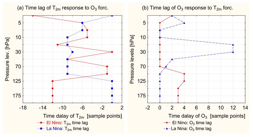
Remote Sens. 2022, 14, 1429                                                                                            9 of 15

                                    Figure 3a illustrates the ozone-pressure covariance (with O3 as leading variable).
                              Note that there are three centers of ozone impact on the pressure—in the tropical central
                              Pacific, over Australia, and over South Africa. Analysis of the time lags (bottom left panel
                              in Figure 3a) shows that variations of the lower stratospheric ozone, during the El Niño
                              phase, precede the changes in the sea level pressure by 2–4 samples’ time intervals. The two
                              tests of significance, of calculated correlation coefficients, provide a confidence that ozone
                              variations near 70 hPa influence temporal variation of the tropical air surface temperature
                              near the date line (refer to the 4th line in Table 1).
                                    The opposite effect (i.e., the surface pressure influence on the ozone at 70 hPa) is well
                              detected near the northern coasts of the Indian Ocean and in the North Pacific Ocean, with
                              the ozone response delayed by 1–5 record’s time intervals (see the right panels in Figure 3).
                                    During La Niña episodes, the ozone–pressure correlation is significantly weakened
                              (Figure 4), especially the pressure influence on ozone, which is reported by other authors
                              as well. The time delay of ozone response in the Indo-Pacific region is highly increased
                              (Figure 4d), which affects the value of correlation coefficients (preliminary weighted by
                              the autocorrelation function of the sea surface pressure, with shift in time corresponding to
                              the ozone time lag). The center of ozone impacts on the pressure in the La Niña phase is
                              also weakened, and moved poleward at subtropical or extratropical latitudes compared
                              to its strength and position during the El Niño episodes. Nevertheless, the two methods
                              for hypothesis testing confirm with 95% confidence that the maximal ozone–temperature
                              correlation is significantly different from zero (refer to the last row in Table 1).
                                    Due to the fact that the ozone response to ENSO variability is well investigated, our
                              further analysis will be concentrated on the changes in the lower stratospheric ozone,
                              preceding the phase transition of ENSO. Figure 5 illustrates the averaged distribution of
                              temperature and ozone dynamical anomalies during the period 1900–2019 separately for
                              La Niña and El Niño composites. Dynamical anomalies illustrate the deviations of monthly
                              T2m and O3 values from the non-stationary (but dynamically evolving from decade to
                              decade) records’ means. The mean values of ozone anomalies are close to zero for both
                              composites. The El Niño mean, however, is slightly negative (i.e., −0.01261), while that
                              of La Niña is slightly positive (i.e., 0.01352). Estimated confidence intervals reveal that all
                              positive La Nina anomalies greater than 0.0144 and all negative anomalies are significantly
                              different from zero with a 95% confidence. Similarly, El Nino anomalies, which are smaller
                              than −0.0138, as well as all positive anomalies, are significantly different from the near
                              zero mean at the 95% confidence level.
                                    Analysis of the mean values of temperature anomalies reveals that during the warm
                              ENSO phase the air surface temperature is systematically biased toward higher values
                              (mean dT2m = 0.1624). Conversely, the temperature during the La Niña phase is generally
                              lower (mean dT2m = −0.1094). Coloured in Figure 5 are the only results confidently different
                              from zero anomalies, which for the air temperature are correspondingly (dT2m < 0; dT2m >
                              0.1694) for El Nino, and (dT2m < −0.11545; dT2m > 0) for the La Niña phase.
                                    It is worth noting that depletion of the lower stratospheric ozone during the warm
                              El Niño episodes, which has been noticed previously in shorter time records, has been
                              persistent for more than a century (Figure 5d). Conversely, during the La Niña episodes,
                              the ozone density is higher than the non-linear sample’s mean (Figure 5c). Usually, this
                              difference is attributed to the strengthening of the Brewer–Dobson circulation during
                              the warm ENSO phase [20]. However, our analysis of the temporal synchronization
                              between ozone at 70 hPa and sea level pressure variations illustrates that during the El
                              Niño phase the ozone variability precedes the changes of sea–surface pressure by 2–4
                              record’s time intervals (see Figure 3). The impact is strongest in the tropical central Pacific
                              (refer to dashed contours in Figure 5d).
Remote Sens. 2022, 14, 1429 10 of 15
Figure 5. Spatial distribution of dynamical anomalies of air surface temperature (a,b) and ozone at 70
hPa (c,d), covering the period 1900–2019, are shown for La Niña (a,c) and El Niño (b,d) composites.
The ozone–sea level pressure correlation, shown in Figure 3, (with O3 as the leading factor), is overlaid
on the maps of ozone anomalies for easier comparison.
The discovery of the central Pacific El Niño [1–3], with its increased frequency of
occurrence since the beginning of the 21st century, motivated us to compare the ozone time
series in predominantly warm or cold ENSO phases during several two-year intervals. Two
decades have been selected for comparison—the period 1980–1989, which is characterized
by classical El Niño events—and the 2000–2011 decade, when the central Pacific El Niño is
quite frequent.
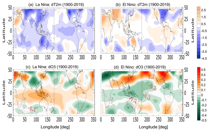
Biennial time series of equatorial ozone at 70 hPa, at the longitude of its strongest
coupling with the sea level pressure (i.e., at 10◦ N and 190◦ E), are presented in Figure 6. It is
well visible that La Niña episodes (blue curves) are characterized by slightly higher ozone
density at 70 hPa, compared to the El Niño episodes (red curves). For easier discrimination
between both ENSO phases, the corresponding values of the standardized Nino3.4 index are
shown in the right column. Comparison of top and bottom panels of Figure 6 (left column)
illustrates that the decade with a higher frequency of the Central Pacific El Niño events
(i.e., 2000–2011) shows the more distinct difference in ozone density between cold and
warm ENSO phases.Remote Sens. 2022, 14, 1429 11 of 15
Figure 6. Two year time series of ozone at 70 hPa (left column) and Nino3.4 index (right column)
corresponding to La Niña (blue curves) and El Niño (red curves), for two decades: 1980–1989
(top panels) and 2000–2011 (bottom ones).
The spatial distribution of ozone changes—from 1980–1989 decade, to 2010–2019 one—
is shown in Figure 7. The statistical significance of differences between ozone values in both
decades has been estimated by the use of Student’s t-test, which compares the means of
both records. The F-test for equality/non-equality of the variances is incorporated in the t-
test provided by the STATISTICA software. The results show that the difference between
the ozone mixing ratio within the 1980s and 2010s is statistically significant at the 95% level
for the La Nina sample, and at the 90% level for the El Nino record.
Figure 7. Multidecadal changes of the lower stratospheric ozone mixing ratio, calculated as a differ-
ence between the decades 2010–2019 and 1980–1989, discriminated between for La Niña (left panel)
and El Niño episodes (right panel).Remote Sens. 2022, 14, 1429 12 of 15
The stronger depletion of equatorial ozone near the dateline, compared to the eastern
and western edges of the tropical Pacific Ocean, is clearly visible during the El Niño phase
(see Figure 7). Within the framework of our hypothesis for the lower stratospheric ozone
influence on climate (e.g., [9,17]), this means a greater warming of the Central Pacific region
and less one sideways (for a brief explanation of the mechanism of ozone influence, see
the next section). Consequently, the spatial distribution of the lower stratospheric ozone
in recent decades could be a good explanation of the ‘strange’ behaviour of the ENSO cycle,
manifesting itself as Central Pacific El Niño events.
3.3. Statistical Analysis of the Tropical Central Pacific Ozone Profile and the Air Surface
Temperature
This section investigates the altitude dependence of air temperature coupling with
ozone density at different levels above the surface. The strength of the relation has been
estimated by the use of the lagged cross-correlation analysis. ERA interim reanalysis—
which has reliably incorporated the satellite data for the ozone profile since 1979—have
been used in this analysis. Two composites have been constructed, for the La Niña and El
Niño phases, using the monthly values of ozone in the tropical Central Pacific (at point
with coordinates 10◦ N; 170◦ W, where the ozone–pressure correlation has its maximal
values—see Figure 3a). The results are presented in Figures 8 and 9.
Figure 8a shows that the ozone impact on the near surface temperature (T2m ), which
is particularly stronger at 70 hPa, corresponds to its increased density at this level during
La Niña episodes (refer to Figure 7). The opposite, i.e., the T2m influence on the ozone, is
detected only during the La Niña phase, being positive in the middle stratosphere and
negative in the lower stratosphere. The absolute value of correlation coefficients at 50–70
hPa with ozone as a responder (Figure 8b), matches the ones calculated with the ozone
as a leading factor (Figure 8a). This result puts the question about the causality between
the lower stratospheric ozone and the near-surface temperature (particularly in this altitude
interval), which could be resolved by an analysis of the time lag of the dependent variable.
Figure 8. Cross-correlation coefficients of ozone profile in the Central Pacific (10◦ N, 170◦ W) with
the temperature at 2 m above the surface (T2m ), calculated for the period 1979–2019. The forcing
factor in (a) panel is ozone, while in (b)—the T2m . The zero lag correlation (the black line), which is
the strongest one, is not suitable to infer the causality of the O3 -T2m relation.Remote Sens. 2022, 14, 1429 13 of 15
Figure 9. Time delay of the near surface temperature (T2m ) response to ozone changes (a), together
with the ozone response to the T2m forcing (b), in relative records’ units of time.
The time delay of the T2m response to O3 forcing, as well as the ozone response to
the temperature forcing, is shown in Figure 9. Note that the surface temperature cooling
in the cold ENSO phase is delayed by 9 samples’ time intervals, since the moment of
the lower stratospheric ozone enhancement (the blue curve in Figure 9a). This lag is long
enough for any physical meaning; moreover, the analysed time records are composites
of consecutive La Nina events, which may belong to different years. On the other hand,
the ozone’s response at 70–50 hPa to the colder sea surface is only 1–2 record’s time
intervals (blue curve in Figure 9b). This result suggests that the enhancement of the lower
stratospheric ozone, initiating a cooling of the surface temperature during La Niña, is
strengthened additionally by the reduced vertical upwelling of the upper troposphere to
the lower stratosphere [19].
The strength of the lower stratospheric O3 influence on the air surface temperature is
slightly weaker during the El Niño episodes (red curve in Figure 8a), but the time delay of
the T2m response is only 1 record’s time interval. This result suggests that surface warming,
initiated by the ozone depletion at 70 hPa, develops much faster than the surface cooling
initiated by the O3 enhancement. One explanation of this delayed surface cooling could be
the time necessary for the upper tropospheric dehydration, initiated by the stably stratified
atmosphere. The influence of the warmer sea surface on stratospheric ozone (during the El
Niño) could not be certainly established, because the strongest temperature–ozone correla-
tion (the black curve in Figure 8) is without time lag (refer to Figure 9b). The mechanism of
such an influence is widely discussed in the scientific literature (e.g., [16–18]) and will not
be considered here.
The chain of relations mediating the ozone influence on the near surface temperature,
however, is less known. Therefore, we will present it to the reader’s attention (for exhaustive
details see [9]). In brief it could be summarised as follows: the lower stratospheric ozone
modulates the temperature and humidity in the upper troposphere, which in turn affects
the strength of the water vapour greenhouse warming. For example, ozone depletion cools
the near-tropopause region, making the upper troposphere more unstable [22]. The upward
propagation of the more humid air masses from the lower atmospheric levels moistens
the upper troposphere and strengthens the greenhouse warming of the planet. The satellite
measurements show that water vapour at these levels ensures 90% of the greenhouse
warming imposed by the total atmospheric humidity [23]. Consequently, the depleted
ozone near the dateline will be projected on the sea surface as temperature warming.Remote Sens. 2022, 14, 1429 14 of 15
The extra warming of the Central tropical Pacific stimulates the eastward movement of
the Walker circulation and a weakening of the trade winds, triggering in such a way
the appearance of the warm ENSO phase [5]. Conversely, the enhancement of the lower
stratospheric ozone density warms the tropopause and stabilises the upper troposphere—
thus putting it in a mode of gradual dehydration [19]. The impact of the dry upper
troposphere in the greenhouse warming is minimal, which explains the disappearance of
the ozone–sea level pressure covariance during the La Niña episodes (see Figure 4).
4. Conclusions
Analysis of the spatial–temporal evolution of the lower stratospheric ozone, air surface
temperature and sea surface pressure, reveals their covariance at different time scales.
The strength of the synchronisation is irregularly distributed across the globe. The tropical
Pacific Ocean was in the focus of this research due to its high variability and significant
impact in the regional climatic changes.
At interdecadal time scales, we found a significant imprint of the 70 hPa ozone
variability over the Nino3.4 index, in the tropical Central Pacific region. The ozone signal
has been detected also at subdecadal time scales as a synchronous temporal variability
with the subtropical air surface temperature, particularly in the area of interest, i.e., near
the dateline meridian, tropical Indian Ocean and the Maritime Continent.
Comparison of ozone’s variability at an interannual time scale, with the one of the sea
level pressure, reveals existing synchronisation with different strength during El Nino and
La Nina episodes. Besides, the well-known effect of El Niño sea level pressure influence
on the ozone (which was strongest near the northern coast of the Indian Ocean, North Pacific
and North Atlantic Oceans), we found also an opposite one, i.e., ozone influence on the sea
level pressure. The strongest ozone–pressure relation has been detected in the tropical
Central Pacific, during the warm ENSO phase—El Niño, with a time lag of pressure
response of 1–2 record’s time intervals (unevenly distributed on the time axis).
Analysis of the near surface temperature sensitivity to changes at different levels of
the ozone profile confirms the importance of ozone variations near 70 hPa. We found that
the raise of ozone density at these levels could trigger a cooling of the tropical Central Pacific
Ocean with a delay of 9 record’s time units. The feedback of the colder sea surface during La
Niña events is projected backward on the lower stratospheric levels via ozone enhancement
(due to the reduced Brewer–Dobson circulation), with a delay of 1–2 record’s units.
The ozone impact on the El Niño surface temperature in the tropical Central Pacific is
a bit weaker, but the temperature responds with a delay of only 1 record’s point. The op-
posite effect, i.e., a causal temperature influence on the stratospheric ozone, could not be
certainly detected, because of the zero-lag of the ozone response.
In conclusion, the spatial–temporal variations of the ozone in the tropical lower strato-
sphere are able to initiate not only the phase transition between ENSO phases, but also its
variability on subdecadal and interdecadal time scales. This conclusion raises the reason-
able question of the driver of ozone variability in the lower stratosphere. In our previous
research, we argue that such variability could be attributed to the existence of a secondary
source of ozone in the lower stratosphere, initiated there by the ion-molecular reactions
in the dry lower stratosphere, and irregularly distributed ionisation in the Regener–Pfotzer
maximum, triggering these reactions [24].
Author Contributions: Conceptualization, N.A.K.; methodology, N.A.K.; software, N.A.K.; vali-
dation, T.P.V.; formal analysis, T.P.V.; investigation, T.P.V.; resources, E.A.B.; data curation, N.A.K.;
writing—original draft preparation, N.A.K.; writing—review and editing, N.A.K., E.A.B.; visualiza-
tion, T.P.V.; project administration, E.A.B.; funding acquisition, E.A.B. All authors have read and
agreed to the published version of the manuscript.
Funding: This research was funded by National Science Fund of Bulgaria Contracts KP-06-N34/1
/30-09-2020, and DN 14/1 from 11.12.2017.Remote Sens. 2022, 14, 1429 15 of 15
Acknowledgments: The authors are sincerely grateful to the project teams of ERA 20 Century and
ERA Interim reanalyses, providing gridded data for ozone temperature and pressure. We also thank
Trenberth, Kevin and the National Centre for Atmospheric Research Staff, for providing “The Climate
Data Guide: Nino SST Indices (Nino 1+2, 3, 3.4, 4; ONI and TNI)”.
Conflicts of Interest: The authors declare no conflict of interest.
References
1. Fu, C.; Diaz, H.F.; Fletcher, J.O. Characteristics of the response of sea surface temperature in the central Pacific associated with
warm episodes of the Southern Oscillation. Mon. Weather Rev. 1986, 114, 1716–1739. [CrossRef]
2. Larkin, N.K.; Harrison, D.E. On the definition of El Niño and associated seasonal average U.S. weather anomalies. Geophys. Res.
Lett. 2005, 32, L13705. [CrossRef]
3. Ashok, K.; Behera, S.K.; Rao, S.A.; Weng, H.; Yamagata, T. El Niño Modoki and its possible teleconnection. J. Geophys. Res. Ocean.
2007, 112, C11007. [CrossRef]
4. Yeh, S.-W.; Kug, J.-S.; Dewitte, B.; Kwon, M.-H.; Kirtman, B.P.; Jin, F.-F. El Niño in a changing climate. Nature 2009, 461, 511–514.
[CrossRef] [PubMed]
5. Gerald, R.; John, N.; Pyle, A.; Zhang, F. (Eds.) Encyclopedia of Atmospheric Sciences, 2nd ed.; Academic Press: Cambridge, MA,
USA, 2015; ISBN 9780123822260.
6. Yang, S.; Li, Z.; Yu, J.-Y.; Hu, X.; Dong, W.; He, S. El Niño–Southern Oscillation and its impact in the changing climate. Natl. Sci.
Rev. 2018, 5, 840–857. [CrossRef]
7. Lin, J.; Qian, T. Switch Between El Nino and La Nina is Caused by Subsurface Ocean Waves Likely Driven by Lunar Tidal Forcing.
Sci. Rep. 2019, 9, 13106. [CrossRef] [PubMed]
8. Manatsa, D.; Mukwada, G. A connection from stratospheric ozone to El Niño-Southern Oscillation. Sci. Rep. 2017, 7, 5558.
[CrossRef] [PubMed]
9. Kilifarska, N.A.; Bakhmutov, V.G.; Malnyk, G.V. The Hidden Link Between Earth’s Magnetic Field and Climate, 1st ed.; Elsevier:
Amsterdam, The Netherlands; Oxford/Cambridge UK, 2020; 218p.
10. Velichkova, T.; Kilifarska, N. Inter-Decadal Variations of the Enso Climatic Mode and Lower Stratospheric Ozone. C. R. l’Acad.
Bulg. Sci. 2020, 73, 539–546.
11. Box, G.E.P.; Jenkins, G.M. Time Series Analysis: Forecasting and Control; Holden-Day: San Francisco, CA, USA, 1976.
12. Afyouni, S.; Smith, S.M.; Nichols, T.E. Effective degrees of freedom of the Pearson’s correlation coefficient under autocorrelation.
NeuroImage 2019, 199, 609–625. [CrossRef] [PubMed]
13. Anderson, O.D. Time Series Analysis, Theory and Practice; North-Holland: Amsterdam, The Netherlands, 1983; Volume 7.
14. Pyper, B.J.; Peterman, R.M. Comparison of Methods to Account for Autocorrelation in Correlation Analyses of Fish Data. Can. J.
Fish. Aquat. Sci. 1998, 2140, 2127–2140. [CrossRef]
15. Kenny, D.A. Correlation and Causality; John Wiley & Sons Inc.: New York, NY, USA, 1979.
16. Jing, P.; Cunnold, D.M.; Yang, E.-S.; Wang, H.-J. Influence of isentropic transport on seasonal ozone variations in the lower
stratosphere and subtropical upper troposphere. J. Geophys. Res. Atmos. 2005, 110, D10110. [CrossRef]
17. Kilifarska, N.A. Mechanism of lower stratospheric ozone influence on climate. Int. Rev. Phys. 2012, 6, 279–290.
18. Solomon, A.; Jin, F.-F. A Study of the Impact of Off-Equatorial Warm Pool SST Anomalies on ENSO Cycles. J. Clim. 2005, 18,
274–286. [CrossRef]
19. García-Herrera, R.; Calvo, N.; Garcia, R.R.; Giorgetta, M.A. Propagation of ENSO temperature signals into the middle atmosphere:
A comparison of two general circulation models and ERA-40 reanalysis data. J. Geophys. Res. Atmos. 2006, 111, D06101. [CrossRef]
20. Calvo, N.; Garcia, R.R.; Randel, W.J.; Marsh, D.R. Dynamical Mechanism for the Increase in Tropical Upwelling in the Lowermost
Tropical Stratosphere during Warm ENSO Events. J. Atmos. Sci. 2010, 67, 2331–2340. [CrossRef]
21. Randel, W.J.; Garcia, R.R.; Calvo, N.; Marsh, D. ENSO influence on zonal mean temperature and ozone in the tropical lower
stratosphere. J. Geophys. Res. 2009, 36, L15822. [CrossRef]
22. North, G.R.; Eruhimova, T.L. Atmospheric Thermodynamics: Elementary Physics and Chemistry; Cambridge University Press:
Cambridge, UK, 2009.
23. Inamdar, A.K.; Ramanathan, V.; Loeb, N.G. Satellite observations of the water vapor greenhouse effect and column longwave
cooling rates: Relative roles of the continuum and vibration-rotation to pure rotation bands. J. Geophys. Res. Atmos. 2004, 109,
D06104. [CrossRef]
24. Kilifarska, N.A. Hemispherical asymmetry of the lower stratospheric O3 response to galactic cosmic rays forcing. ACS Earth Space
Chem. 2017, 1, 80–88. [CrossRef]You can also read