Fort Laramie National Historic Site Plant Community Composition and Structure Monitoring
←
→
Page content transcription
If your browser does not render page correctly, please read the page content below

National Park Service
U.S. Department of the Interior

Natural Resource Stewardship and Science

Fort Laramie National Historic Site Plant
Community Composition and Structure
Monitoring
2011 Annual Report
Natural Resource Technical Report NPS/NGPN/NRTR—2012/536
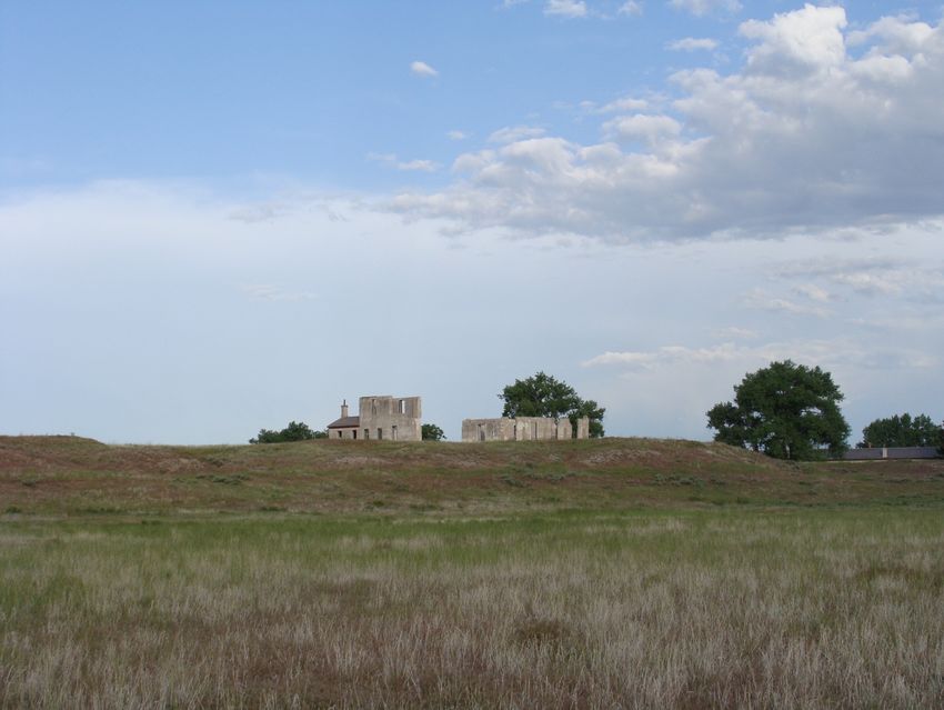
ON THE COVER
A view of a Fort Laramie National Historic Site, 2011
Photograph by: Belinda Lo, NGPN, NPS
Fort Laramie National Historic Site Plant
Community Composition and Structure
Monitoring
2011 Annual Report
Natural Resource Technical Report NPS/NGPN/NRTR—2012/536

Isabel W. Ashton
Michael Prowatzke
Michael R. Bynum
Tim Shepherd
Stephen K. Wilson
Kara Paintner-Green

National Park Service
Northern Great Plains Inventory & Monitoring Network
231 East Saint Joseph St.
Rapid City, SD 57701

February 2012

U.S. Department of the Interior
National Park Service
Natural Resource Stewardship and Science
Fort Collins, Colorado

The National Park Service, Natural Resource Stewardship and Science office in Fort Collins,
Colorado publishes a range of reports that address natural resource topics of interest and
applicability to a broad audience in the National Park Service and others in natural resource
management, including scientists, conservation and environmental constituencies, and the public.

The Natural Resource Technical Report Series is used to disseminate results of scientific studies
in the physical, biological, and social sciences for both the advancement of science and the
achievement of the National Park Service mission. The series provides contributors with a forum
for displaying comprehensive data that are often deleted from journals because of page
limitations.

All manuscripts in the series receive the appropriate level of peer review to ensure that the
information is scientifically credible, technically accurate, appropriately written for the intended
audience, and designed and published in a professional manner.

Data in this report were collected and analyzed using methods based on established, peer-
reviewed protocols and were analyzed and interpreted within the guidelines of the protocols.

Views, statements, findings, conclusions, recommendations, and data in this report do not
necessarily reflect views and policies of the National Park Service, U.S. Department of the
Interior. Mention of trade names or commercial products does not constitute endorsement or
recommendation for use by the U.S. Government.

This report is available from Northern Great Plains Network website
(http://science.nature.nps.gov/im/units/ngpn/reportpubs/reports.cfm) and the Natural Resource
Publications Management website (http://www.nature.nps.gov/publications/nrpm/).

Please cite this publication as:

Ashton, I. W., M. Prowatzke, M. Bynum, T. Shepherd, S. K. Wilson, K. Paintner-Green. 2012.
Fort Laramie National Historic Site plant community composition and structure monitoring:
2011 annual report. Natural Resource Technical Report NPS/NGPN/NRTR—2012/536. National
Park Service, Fort Collins, Colorado.

NPS 375/112634, February 2012

                                                 ii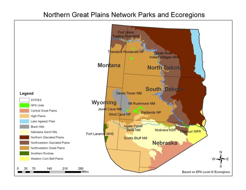
Contents
                                                                                                                                               Page

Figures............................................................................................................................................. v

Tables .............................................................................................................................................. v

Executive Summary ...................................................................................................................... vii

Acknowledgments........................................................................................................................ viii

Introduction ..................................................................................................................................... 1

Methods........................................................................................................................................... 3

      Sample design .......................................................................................................................... 3

      Plot layout and sampling ......................................................................................................... 5

           Establishing, Marking, and Photographing Long-term Monitoring Plots .......................... 5

           Plant Sampling .................................................................................................................... 7

      Data Management and Analysis .............................................................................................. 9

Results ........................................................................................................................................... 11

      Absolute percent and relative cover ...................................................................................... 11

      Species richness, diversity, and evenness .............................................................................. 11

      Forest structure and surface fuels .......................................................................................... 12

      Target species assessments and disturbance .......................................................................... 13

Discussion ..................................................................................................................................... 15

Literature Cited ............................................................................................................................. 17

Appendix A: Field journal for plant community monitoring in FOLA for the 2011
season ............................................................................................................................................ 19

Appendix B: List of plant species found in 2011 at FOLA .......................................................... 21

                                                                         iii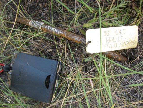
Figures
Page
Figure 1. Parks and ecoregions of the Northern Great Plains Network. ........................................ 1
Figure 2. Map of FOLA and plant community monitoring plots................................................... 4
Figure 3. [2-3] revisit design for intensive plant community composition and
structure monitoring at most NGPN parks...................................................................................... 5
Figure 4. Layout for NGPN intensive plant community composition and structure
plots. ................................................................................................................................................ 6
Figure 5. A sample of the center marker at an NGPN long-term vegetation
monitoring plot. .............................................................................................................................. 7
Figure 6. A sample of tags and washers used to mark long-term vegetation
monitoring plots in the NGPN. ....................................................................................................... 7
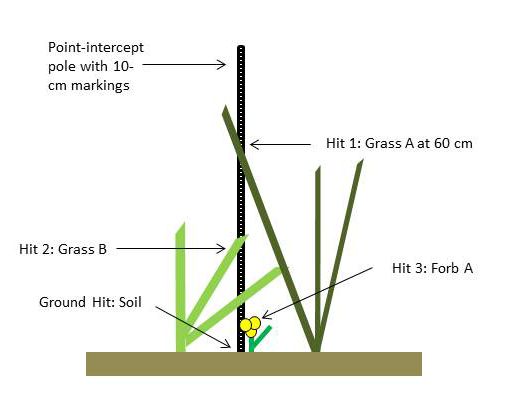
Figure 7. The NGPN point-intercept method captures multiple layers of the plant
canopy. ............................................................................................................................................ 8
Figure 8. Arrangement of nested quadrats along tape used for point-intercept
sampling. ......................................................................................................................................... 9
Figure 9. Absolute percent cover of different plant life-forms in 5 plant community
monitoring plots in FOLA in 2011. .............................................................................................. 12
Figure 10. The woody riparian plant community monitoring plot sampled in 2011 by
NGPN............................................................................................................................................ 13
Tables
Page
Table 1. Target species in FOLA for the 2011 field season. .......................................................... 9
Table 2. Average plant species richness at 5 plots at FOLA in 2011. ......................................... 12
Table 3. Natural resource condition summary table for plant communities in FOLA................. 16
vExecutive Summary
The Northern Great Plains Inventory & Monitoring Network (NGPN) was established to develop
and provide scientifically credible information on the current status and long-term trends of the
composition, structure, and function of ecosystems in thirteen parks located in 5 northern Great
Plains states. NGPN identified upland plant communities, exotic plant early detection, and
riparian lowland communities as vital signs that can be used to better understand the condition of
terrestrial park ecosystems. Upland and riparian ecosystems are important targets for vegetation
monitoring because the status and trends in plant communities provide critical insights into the
status and trends of other biotic components within those ecosystems.
In 2011, NGPN began plant community monitoring in Fort Laramie National Historic Site
(FOLA). We visited 5 long-term monitoring plots on June 13-16th, 2011, and recorded a total of
84 vascular plant species. This effort was the first year in a multiple-year venture to understand
the status of upland and riparian lowland plant communities in FOLA. At the end of 5 years,
there will be an in-depth report describing the status of the plant community. In this report, we
provide a simple summary of our results from sampling in 2011. We found the following:
• Absolute vascular plant cover was high due to a wet spring, and grasses and sedges made
up the bulk of vascular plant cover at all sites.
• The sites at FOLA had a low to moderate diversity of vascular plants compared to other
grasslands in the network. Average native species richness in the 10 m2 quadrats was 7 ±
3.6 species (mean ± standard deviation).
• Exotic species occurred in all plots we visited and the relative cover of exotics species
was 54% across the plots. Houndstongue and Scotch thistle were the only 2 target exotic
species we encountered and they were found in only 1 site in low abundance.
viiAcknowledgments We thank all the authors of the NGPN Plant Community Monitoring Protocol, particularly Amy Symstad for outstanding guidance on data collection and reporting. We thank the Northern Great Plains Fire Management team for ongoing assistance with fieldwork and development of methods. We greatly appreciate the staff at FOLA for providing logistical support. The 2011 NGPN vegetation field crew of Belinda Lo, Ryan Manuel, Lee Margadant, and Kara Paintner- Green, collected all the data included in this report. We thank Timothy Shepherd for invaluable support and instruction on managing data in the FFI database and Stephen Wilson for assistance with the GIS data.
Introduction
One of the objectives of the National Park Service (NPS) Inventory & Monitoring (I&M)
Program is to develop and provide scientifically credible information on the current status and
long-term trends of the composition, structure, and function of park ecosystems, and to
determine how well current management practices are sustaining those ecosystems. The
Northern Great Plains I&M Network (NGPN) includes 13 parks located in 5 northern Great
Plains states across 6 ecoregions (Figure 1) and vary widely in size, amount of visitor use, and
management context.

Figure 1. Parks and ecoregions of the Northern Great Plains Network. Based on the U.S. Environmental
Protection Agency’s Level III ecoregions classes (Omernik 2007).

NGPN identified upland plant communities, exotic plant early detection, and riparian lowland
communities as vital signs that can be used to better understand the condition of terrestrial park
ecosystems (Gitzen et al. 2010). Network-wide land cover is dominated by native upland
grassland, but some small parks are dominated by old fields and recent prairie plantings
(Symstad et al. 2011). Other major land cover types include barren or sparsely vegetated areas
(Badlands and Theodore Roosevelt national parks) and ponderosa pine forests and woodlands in
Black Hills parks. Riparian hardwood forests comprise a small portion of the area but have
disproportionately large ecological significance because of their value to wildlife species.

                                                  1
The NGPN selected upland and riparian ecosystems as an important vegetation monitoring target because knowing the status and trends in plant communities of any terrestrial ecosystem is critical to understanding the status and trends in most other biotic components of that ecosystem. Not only are plants the source of food for most organisms, but they also provide other organisms cover from predators and the elements, structure for basic life-history processes (e.g., nest sites), and substrate on which to grow. Plant communities influence local, regional, and global climate through evapotranspiration, albedo, and greenhouse gas emissions and absorption (Smith et al. 1997). Fire regimes (D'Antonio and Vitousek 1992) and flood behavior (Anderson et al. 2006) are in part mediated by the species that comprise plant communities and the structure that they create. Plants are the major source of organic inputs into soil and aquatic systems. Finally, vegetation is a large part of the scenery that visitors to NPS units come to enjoy. The long-term objectives of our plant community monitoring effort (Symstad et al. 2011) in FOLA are to: 1. Determine park-wide status and long-term trends in vegetation species composition (e.g., non-native vs. native, forb vs. graminoid vs. shrub) and structure (e.g., cover, height) of herbaceous and shrub species. 2. Determine status (at 5-year intervals) and long-term trends of tree density tree density by species, height class, and diameter class in lowland riparian areas. 3. Improve our understanding of the effects of external drivers and management actions on plant community species composition and structure by correlating changes in vegetation composition and structure with changes in climate, landscape patterns, atmospheric chemical composition, fire, and invasive plant control. This report is intended to provide a timely release of basic data sets and data summaries for our initial sampling efforts in 2011 at FOLA. We visited 5 plots in a rotating panel design and it will take 4 more years to visit every plot in the park. We expect to produce reports with more in- depth data analysis and interpretation when we complete 5 years of sampling (i.e., visit and sample every plot in the park twice, following a rotating panel design that stipulates 2 years of visitation and 3 years of rest per 5-year period). In 2014, we will conduct a large effort to examine riparian forest structure and health in FOLA where we will visit 20 forested plots. Reports, spatial data, and data summaries can also be provided as needed for park management and interpretation.
Methods
The NGPN Plant Community Composition and Structure Monitoring Protocol (Symstad et al.
2011) describes in detail the methods used for sampling upland and riparian vegetation in 11
parks of the network. Below, we briefly describe the general approach, sample frame, plot
locations, and sampling methods. For those interested in more detail, please see Symstad et al.
2011, available at http://science.nature.nps.gov/im/units/ngpn/monitor/plants/plants.cfm .

Sample design
NGPN has implemented a survey to monitor vegetation in FOLA using a Generalized Random
Tessellation Stratified (GRTS) sampling design (Stevens and Olsen 2003, 2004). Probability-
based surveys provide unbiased estimation of both status and, with repeated visits, trend across a
resource (Larsen et al. 1995). When implemented successfully, probability-based survey designs
allow for unbiased inference from sampled sites to un-sampled elements of the resource of
interest (Hansen et al. 1983). The goal of our probability-based design is to determine the status
of vegetation after 5 years and from then on, the trend in vegetation.

The methods for the development of the survey design and site selection are described in detail
in Symstad et al. 2011. In brief, a probability-based survey design consists of implementing the
following steps prior to field sampling: defining a resource or target population and any
subpopulations of interest, creating a sample frame within the target population, selecting sites to
visit within the sample frame, and determining when to sample. For FOLA, we define the target
population as vegetation in the entire park and the sample frame as all vegetation. Riparian
lowland areas and upland areas are unique stratum because the management importance of
riparian lowlands is disproportionate to area. For all parks, we exclude the following areas from
the sample frame: administrative areas, roads, canals, or utility lines and an appropriate buffer,
areas within 10 m of a park boundary, paved trails, areas with little to no potential for terrestrial
vegetation (e.g. large areas of bare rock), areas that are dangerous of prohibitively difficult to
access or work on, and areas that are not owned by the park. The final design includes 5
randomly located riparian sites and 10 randomly located upland sites representing the park where
vegetation will be sampled close to peak phenology (mid June) (Figure 2).

An ideal revisit design would consist of a large number of sites distributed throughout a park
being sampled every year. Limited resources, as well as the danger of plot wear-out (trampling
and other effects of sampling), precluded this design. Instead, NGPN intensive plant community
composition and structure monitoring uses a connected [2-x] rotating-panel design: every park is
visited every year, but sites are grouped into panels where each panel (and the plots therein) is
measured for 2 consecutive years followed by 3 or more years without sampling. Because only a
subset of panels (and therefore plots) are visited each year, this allows more sites than can be
visited in one year to be included in the sample design, while including revisitation of sites to
address annual variability. Compared to the always-revisit design, connected panel designs, in
which each panel is revisited periodically, sacrifice little power for detecting trend (Urquhart and
Kincaid 1999) but provide much greater spatial coverage, and thus improved precision in
estimates of status. At FOLA, we will visit 2 panels each with 3 sites every year and after 5 years
we will have visited all sites twice (Figure 3). In 2011, we visited sites in panel 1 and panel 5
(Figure 2).
Figure 2. Map of FOLA and plant community monitoring plots. Plots in Panel 1 (orange) and Panel 5 (purple) were visited in 2011.

                                                                       4
Year↓ / Panel→ P1 P2 P3 P4 P5
2011 3 3
2012 3 3
2013 3 3
2014 3 3
2015 3 3
2016 3 3
2017 3 3
2018 3 3
2019 3 3
2020 3 3
2021 3 3
Figure 3. [2-3] revisit design for intensive plant community composition and structure monitoring at most
NGPN parks. Five panels are used in a park or stratum. Data are collected in the plots of a given panel, 2
of every 5 years. Blank cells indicate no plots in the panel are visited that year; at FOLA there are 3 plots
in a panel (1 riparian and 2 upland plots). Thus, 6 plots (2 panels) are sampled each year and the total
sample size is 15, across all 5 panels.
The number of plots allocated to each park and to strata within parks is influenced by a
combination of factors, including field work logistics, statistical power estimations (see Symstad
et al. 2011), and conformity to the desired revisit design. Plot numbers across parks are allocated
roughly proportional to the size of the sample frame for that park, although the minimum number
of plots per park was set at 15. At FOLA, there are currently 15 monitoring plots. An additional
20 forested riparian plots will be monitored on a separate 5 year schedule starting in 2014.
Plot layout and sampling
The primary sample unit for intensive plant community composition and structure monitoring in
the NGPN consists of a rectangular, 50 m x 20 m (0.1 ha), permanent plot (Figure 4). These are
hereafter referred to as “intensive plots”. In 2011, sampling 5 plots at FOLA took a 4 person
crew approximately 43 hours with travel time (see Appendix A for a detail of activities each
day). One plot, PCM_069, was not sampled because it was flooded. Below, we briefly describe
the methods we used for marking and sampling the plots.
Establishing, Marking, and Photographing Long-term Monitoring Plots
Locations of all intensive plots are determined before monitoring begins in the site evaluation
process. At this time, a single plot marker, marked with a metal tag identifying the plot and the
marker as the center (C), is driven into the ground at the center of the plot (Figure 5). At plot
establishment (which may be done prior to the first visit for data collection), 2 permanent
transects are marked by driving rebar markers into the ground at the end points of each transect.
A metal tag imprinted with the park code, plot ID, corner name (A0, A50, B0, or B50), and
establishment date is attached to each marker. Each transect is also marked with large nails and
5washers sunk flush with the ground at 10.92 m, 23.42 m, 35.92 m, and 46.84 m from the 0 end of
each transect. Figure 6 is a photographic sample of the tags and washers used by NGPN.
At each transect end, a photograph is taken down the length of the transect. When trees and/or
tall shrub species are present in or near the plot, the ends of 2 additional perpendicular, 100-ft
(30.48 m) transects centered at the C plot marker are marked with large nails and washers
(Figure 4). One of these transects (T1) is parallel to the herb-layer transects and the second (T2)
is perpendicular to that transect.
Figure 4. Layout for NGPN intensive plant community composition and structure plots.
6Figure 5. A sample of the center marker at an NGPN long-term vegetation monitoring plot. The rebar is
bent in the field with a brass tag noting the plot number, date of installation, and location. A compass is
used for scale.
Figure 6. A sample of tags and washers used to mark long-term vegetation monitoring plots in the NGPN.
From the top left and working clockwise: a center tag from PCM-08 in SCBL evaluated on May 5, 2009; a
tag used to mark the end of the A transect at WICA PCM-01; a tag used to mark the center of an
extensive plot in MORU; and a washer used to mark the beginning of the second tree transect. In all
cases, the tags are close or flush to the ground. The brass tags are fixed to rebar with wire, and the
washer is held in place by a large nail.
Plant Sampling
Data on ground cover and herb-layer (≤ 2 m height) height and foliar cover were collected on 2
50 m transects (the long sides of the plot) using a point-intercept method at each plot. Starting at
the 0 end of each transect, a 50 m tape was stretched over the length of the transect, ensuring that
it followed the path marked by the nails and washers (Figure 4). At 100 locations along the
transects (every 0.5 m) a pole was dropped to the ground and all species that touched the pole
were recorded, along with ground cover, and the height of the canopy (Figure 7).
7Figure 7. The NGPN point-intercept method captures multiple layers of the plant canopy.
Species richness data from this point-intercept method are supplemented with species presence
data collected in 5 sets of nested square quadrats (0.01 m2, 0.1 m2, 1 m2, and 10 m2; Figure 8)
located systematically along each transect. Nested quadrats are located so that they occur inside
the 20 m x 50 m plot (Figure 4). Beginning with the 0.01 m2 quadrat, all species rooted in the
quadrat are identified and recorded. Once all species in this quadrat are recorded, the observer
moves onto the 0.1 m2 quadrat, listing only species not observed in the 0.01 m2 quadrat. This is
repeated in the 1.0 m2 and 10 m2 quadrats. Only species rooted in a quadrat are included in the
species list for that quadrat.
Unknown species were recorded in the field using a unique identifier and collected or
photographed. Most of these unknowns were subsequently identified by M. Bynum. However, in
some cases the plant was too small or difficult to identify. In these cases, the species was
classified by growth form and, where possible, lifecycle (e.g., annual graminoid).
10 m2
1 m2
0.1 m2
0.01 m2
0 50
8Figure 8. Arrangement of nested quadrats along tape used for point-intercept sampling. Open circle
indicates permanent marker (nail and washer or, at 0 end of transect, rebar).
Where applicable, tree regeneration and tall shrub density data are collected within a 10 m-
radius, circular subplot centered at the center of the 50 m x 20 m plot. In this subplot or a subset
thereof, tree and targeted tall shrub seedlings are tallied by species and size class. Size classes are
defined as follows. A tree has a diameter at breast height (DBH) of greater than 15 cm. A pole
has a DBH of > 2.54 cm but < 15 cm. A sapling has a DBH < 2.54 cm but is > than 1.37 cm tall.
A seedling is < 1.37 cm tall. DBH, status (live or dead), and species are recorded for all poles
and trees and targeted tall shrubs.
Trees with DBH > 15 cm, within the entire 0.1 ha plot, are mapped and tagged, and species,
DBH, status, and condition (e.g., leaf-discoloration, insect-damaged, etc.) are recorded for each
tree. Where appropriate (i.e., in ponderosa pine forest or woodland in Black Hills parks), dead
and downed woody fuel load data are collected on 2 perpendicular, 100 ft (30.48 m) transects
centered at the center of the plot.
At all plots, we also surveyed the area for common disturbances and target species of interest.
Common disturbances included such things as roads, rodent mounds, animal trails, and fire. For
all plots the type and severity of the disturbances were recorded. The target species lists were
developed in cooperation with the park and NGPN staff during the winter/spring prior to the
field season. Usually these are invasive and/or exotic species that are not currently widespread in
the park but pose a significant threat if allowed to establish. For each target species that was
present at a site, an abundance class was given on a scale from 1-5 where 1= one individual, 2=
few individuals, 3 = cover 1-5% of site, 4 = cover 5-25% of site, and 5= cover > 25% of site. The
information gathered from this procedure is critical for early detection and rapid response to such
threats. The FOLA target species list for 2011 can be found in Table 1.
Table 1. Target species in FOLA for the 2011 field season.
Invasives/noxious weeds/exotics
Species Code Scientific Names Common Names
CANU4 Carduus nutans L. Nodding plumeless (musk) thistle
CIAR4 Cirsium arvenseL. Canada thistle
CIVU Cirsium vulgare (Savi) Ten. bull thistle
CYOF Cynoglossum officinale L. Hounds tongue/gypsyflower
ONAC Onopordum acanthium L. Scotch (cotton)thistle
VETH Verbascum thapsus L. common mullein
Data Management and Analysis
After the field work was completed, field sheets were scanned and stored in fire-proof cabinets,
and the data were entered by the NGPN seasonal vegetation crew. FFI (FEAT/FIREMON
Integrated; http://frames.nbii.gov/ffi/) is the primary software environment used for managing
NGPN plant community data. NGPN uses its components for data entry, data storage, and basic
summary reports. FFI is used by a variety of agencies (e.g., NPS, USDA Forest Service, U.S.
Fish and Wildlife Service), has a national-level support system, and generally conforms to the
9Natural Resource Database Template standards established by the Inventory and Monitoring
Program.
Species names, codes, and common names are from the USDA Plants Database (USDA-NRCS
2012). However, nomenclature follows the Integrated Taxonomic Information System (ITIS)
(http://www.itis.gov). In the few cases where ITIS recognizes a new name that was not in the
USDA PLANTS database, the new name was used and a unique plant code was assigned.
After data for the sites were entered, the data were verified. This was done by comparing the
entered data to the original field data sheets, and detected errors were corrected immediately. To
minimize transcription errors, 100% of records were verified to their original source. A further
10% of records were reviewed a second time by I. Ashton or M. Prowatzke. When errors were
found in the reviews, the entire data set was verified again. After all data were entered and
verified, automated queries were developed to check for errors in the data. For instance, a query
was developed that noted all plots where a species appeared twice within one nested quadrat.
When errors were caught by the crew or the automated queries, changes were made to the
original datasheets and the FFI database.
For analysis of data from intensive plots, the plot is used as the unit of replication and quadrats
or transects are pooled or averaged. Data from each plot are summarized for a variety of
variables including: relative cover of growth forms (shrubs, grasses, forbs), absolute cover of
bare soil, total herb-layer foliar cover, density and basal area of trees, species richness and
diversity, relative abundance of functional groups, and proportions of foliar cover and species
richness that are non-native. Growth forms were based on definitions from the USDA Plants
Database. Warm-season grasses were identified primarily using Skinner (2010). Summaries were
done using FFI reports and statistical summaries were done using R software (version 2.11.0).
10Results
In the 5 plots we visited in FOLA during 2011, we recorded 84 vascular plant species (Appendix
B), one additional forb that could not be identified, and one plant that could be identified only to
genus. The most common families were Asteraceae and Poaceae. We visited 1 riparian plot and
4 upland plots. Unless otherwise noted, we present information for all the plots combined
because the low sample size of riparian plots does not warrant separate analyses at this point.
Absolute percent and relative cover
From the point-intercept data, we found plots to average 122 ± 33.6 % (mean ± standard
deviation) total herb layer cover and 19 ± 17.0 % ground layer of bare soil. The absolute canopy
cover can be greater than 100% because we record multiple layers of plants and it was a fairly
wet year with abundant growth.
Graminoids, which includes grasses, sedges, and rushes, had an average absolute cover of 103 ±
33.8%. This was much higher than other plant life-forms (Figure 9). Only 3 species were found
in all 5 sites: 2 grasses, Western wheatgrass (Pascopyrum smithii; 19 ± 14.8 %) and cheatgrass
(Bromus tectorum; 56 ± 34.5 %), and one forb, tall tumblemustard (Sisymbrium altissimum; 3.2
± 2.3 %). A vine, field bindweed (Convolvulus arvensis), was found in only 1 site, but it was
abundant there (17.5% cover).
Of the 5 plots at FOLA, the average relative percent cover of exotic species was 54 ± 21.3 %.
We found the average relative percent cover of warm season graminoids to be 8 ± 5.6 %.
Species richness, diversity, and evenness
We measured diversity at the plots in 2 ways: the Shannon Index and Pielou’s Index of Eveness.
The Shannon Index, H’, is a measure of the number of species in an area and how even
abundances are across the community. It typically ranges between 0 (low richness and evenness)
to 3.5 (high species richness and evenness). Peilou’s Index of Evenness, J’, measures another
aspect of diversity-- how even abundances are across taxa. It ranges between 0 and 1, where
higher numbers indicate that a community is not even or that just a few species make up the
majority of the total cover. From the point-transect data, we found average plot diversity, H’, to
be 1.6 ± 0.33. Evenness, J’, averaged 0.59 ± 0.08 across the plots. When including only native
species, average diversity and evenness were 1.4 ± 0.54 and 0.63 ± 0.20, respectively. Species
richness varies by the scale that it is examined. Table 2 presents average species richness for the
point-intercept, 1 m2 quadrats, and 10 m2 quadrats for the 5 plots in 2011. In general, richness
increases in the larger quadrat size. On average, there are about 6 exotic species found in each
plot along the point-intercept (Table 2).
11Figure 9. Absolute percent cover of different plant life-forms in 5 plant community monitoring plots in
FOLA in 2011. Bars represent means across the 5 plots ± standard errors. Graminoids were the most
abundant plant life-form across all plots at FOLA.
Table 2. Average plant species richness at 5 plots at FOLA in 2011. Values represent means ± standard
deviation.
2 2
Point-intercept 1 m quadrats 10 m quadrats
Species richness 15.8 (4.76) 7.9 (2.62) 11.7 (4.08)
Native species 10.0 (3.54) 4.9 (2.28) 7.4 (3.64)
richness
Exotic species 5.8 (1.64) 3.1 (0.62) 4.3 (0.98)
richness
Graminoid species 6.2 (1.10) 2.8 (0.74) 3.4 (0.89)
richness
Forb species 6.8 (2.39) 4.0 (1.56) 6.3 (2.55)
richness
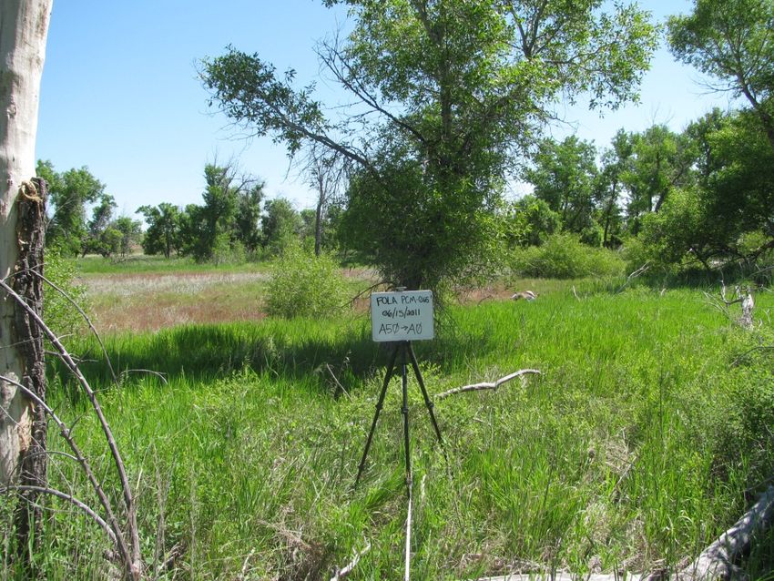
Forest structure and surface fuels
We encountered trees in the single riparian plot we sampled in 2011 (PCM_065; Figure 10). We
measured 4 crack willow (Salix fragilis) and one large live and one dead plains cottonwood
(Populus deltoides ssp. monilifera). We also found a couple of willow and green ash (Fraxinus
pennsylvanica) seedlings.
12Figure 10. The woody riparian plant community monitoring plot sampled in 2011 by NGPN.
Target species assessments and disturbance
Only 2 target species appeared in the plots we visited in 2011: houndstongue and Scotch thistle.
In both cases, only a few individuals were found in PCM_001.
Of the 5 sites at FOLA, 2 showed no evidence of disturbance: PCM_001 and PCM_009. Grazing
was evident at 2 plots (PCM_002, PCM_010) and a large animal trail was present in PCM_065.
In addition to grazing, there was also evidence of pocket gophers and 4-wheel use on PCM_010.
13Discussion
The goal of our plant community monitoring efforts in FOLA is to determine the status and trend
in vegetation composition and structure and to understand how natural and anthropogenic
disturbance and management decisions influence vegetation. As of 2011, we have completed the
first year of field work; while we have increased our understanding of vegetation composition
and structure, we cannot yet describe park-wide status or trends. Below, we summarize the
results from above and highlight some of the most interesting aspects of the plant community
monitoring.
There was considerable variation among plots, but on average bare soil was about 20 % of
ground cover. Absolute vascular plant cover averaged 122 %; productivity was high due to a wet
spring. The sites at FOLA had a low to moderate diversity of vascular plants. Average native
species richness in the 10 m2 quadrats was 7 ± 3.6 species (Table 2). We found an average of 4
exotic plants in every 10 m2 quadrat. Graminoids, which includes all grasses, sedges, and rushes,
made up the bulk of cover at all sites (Figure 9). Forbs, or broad-leaved herbaceous plants, were
less abundant and but generally more diverse than graminoids. Shrubs, vines, and subshrubs
were not a large component of the cover at the sites we visited (Figure 9). Exotics species
occurred in all 5 plots. Relative cover of exotics species was 54% across the plots. While cover
of exotics was high, we found target exotic species in only one plot.
Graminoids can be further classified by their photosynthetic pathway. Warm season graminoids
have a photosynthetic pathway (C4) that particularly adapts them to hot climates and an
atmosphere low in carbon dioxide. These warm season graminoids grow primarily during the hot
summer months and tend to be very drought tolerant. Cool season graminoids are C3 plants that
tend to grow best in cooler temperatures. For example, junegrass (Koeleria macrantha) is a cool
season grass and blue grama (Bouteloua gracilis) is a warm season grass. At these 5 sites, 8 % of
the relative cover was made up of warm-season grasses. Examining the trend over time in warm-
season graminoid cover and climate trends may elucidate whether warm-season grasses are
increasing in abundance due to warmer and drier conditions.
Results from our vegetation monitoring can be summarized in a “connect-the-dots” or a resource
condition summary table (Table 3). These tables can be used to describe the status and trend in
vital signs or other indicators of ecosystem health. We chose a handful of the key metrics
representing 2 vital signs, which we will continue to monitor over time at FOLA. The current
value is based on sampling in 2011 and the level of inference is simply 5 sites. After one
complete rotation in the FOLA sampling design (5 years), current values will be the average
across 5 years and the level of inference will be park-wide. After a minimum of 5 years of data
collection, or one complete rotation in the FOLA panel sampling design, we will also estimate
baseline reference values and begin to estimate trends in these key metrics. Over time, the
vegetation data collected at these sites will greatly add to our understanding and documentation
of change in the upland plant communities at FOLA.
15Table 3. Natural resource condition summary table for plant communities in FOLA.
Vital Sign Metric Current Level of Reference Rationale
Value (mean ± SD) inference Value
% of sites where 20% 5 sites TBD
Early detection of exotic
target species
Exotic Plant species
were encountered
Early
Detection Number of target 0 5 sites TBD
Effectiveness of exotic
species
species management
abundance > 5%
Mean absolute 122 ± 33.6 % 5 sites TBD Forage availability,
herb-layer cover climatic trends, erosion
potential, habitat for
Ground-layer bare 19 ± 17.0 % 5 sites TBD small mammals and
soil cover birds
Upland and Mean relative 54 ± 21.3 % 5 sites TBD
Effectiveness of exotic
Riparian percent cover of
species management
Lowland exotic species
Plant Percent of 8 ± 5.6 % 5 sites TBD
Communities graminoid cover
Climatic trends
that is warm
season
Mean native 7.4 ± 3.64 species 5 sites TBD Diversity maintenance
species richness in
2
10 m quadrats
16Literature Cited
Anderson, B. G., I. D. Rutherfurd, and A. W. Western. 2006. An analysis of the influence of
riparian vegetation on the propagation of flood waves. Environmental Modelling &
Software 21:1290-1296.
D'Antonio, C. M. and P. M. Vitousek. 1992. Biological invasions by exotic grasses, the grass/fire
cycle, and global change. Annual Review of Ecology and Systematics 23:63-87.
Gitzen, R. A., M. Wilson, J. Brumm, M. Bynum, J. Wrede, J. J. Millspaugh, and K. J. Paintner.
2010. Northern Great Plains Network vital signs monitoring plan. Natural Resource
Report NPS/NGPN/ NRR-2010/186.
Hansen, M. H., W. G. Madow, and B. J. Tepping. 1983. An evaluation of model-dependent and
probability-sampling inferences in sample-surveys. Journal Of The American Statistical
Association 78:776-793.
Larsen, D. P., N. S. Urquhart, and D. L. Kugler. 1995. Regional-scale trend monitoring of
indicators of trophic condition of lakes. Water Resources Bulletin 31:117-140.
Omernik, J. M. 2007. Level III Ecoregions of the Continental United States. U.S. EPA National
Health and Environmental Effects Laboratory, Corvallis, Oregon.
Skinner, Q. D. 2010. Field guide to Wyoming grasses. Education Resources Publishing,
Cumming, GA.
Smith, T. M., H.H. Shugart, and F. I. Woodward, editors. 1997. Plant functional types: their
relevance to ecosystem properties and global change. Cambridge University Press,
Cambridge, UK.
Stevens, D. L. and A. R. Olsen. 2003. Variance estimation for spatially balanced samples of
environmental resources. Environmetrics 14:593-610.
Stevens, D. L. and A. R. Olsen. 2004. Spatially balanced sampling of natural resources. Journal
Of The American Statistical Association 99:262-278.
Symstad, A. J., R.A. Gitzen, C. L. Wienk, M. R. Bynum, D. J. Swanson, A. D. Thorstenson, and
K. J. Paintner. 2011. Plant community composition and structure monitoring protocol for
the Northern Great Plains I&M Network: version 1.00. Natural Resource Report
NPS/NGPN/ NRR-2011/291.
Urquhart, N. S. and T. M. Kincaid. 1999. Designs for Detecting Trend from Repeated Surveys of
Ecological Resources. Journal of Agricultural, Biological, and Environmental Statistics
4:404-414.
USDA-NRCS. 2012. The PLANTS Database (http://plants.usda.gov, 24 January 2012). National
Plant Data Team, Greensboro, NC 27401-4901 USA.
17Appendix A: Field journal for plant community monitoring in
FOLA for the 2011 season
Plant community composition monitoring in FOLA was completed using a crew of 4 people
working 4 10-hour days with approximately 4 hours of overtime. Denise Cupp assisted with
sampling on Jun 15th. We sampled 5 plots at FOLA. One plot was not sampled because flood
waters prevented access. The crew drove one vehicle and the total mileage for the trips was 569
miles. We spent a total of 176 crew hours in FOLA in 2011.
Date Day of week Approximate Housing Sites Notes
Travel Time Completed
(hrs)
Jun 13, 2011 Monday 4 Holiday Inn, PCM-001
Torrington, WY
Jun 14, 2011 Tuesday N/A Holiday Inn, PCM-002
Torrington, WY PCM-010
Jun 15, 2011 Wednesday N/A Holiday Inn, PCM-065 1 establishment
Torrington, WY & 1 evaluation
Jun 16, 2011 Thursday 4 N/A PCM-009
19Appendix B: List of plant species found in 2011 at FOLA
Family Code Scientific Name Common Names
Aceraceae ACNEI2 Acer negundo var. interius ash-leaf maple, boxelder, boxelder maple
Anacardiaceae TORY Toxicodendron rydbergii western poison ivy
AMPS Ambrosia psilostachya Cuman ragweed
AMTO3 Ambrosia tomentosa skeletonleaf burr ragweed
ARCA12 Artemisia campestris field sagewort
ARDR4 Artemisia dracunculus tarragon
ARFI2 Artemisia filifolia sand sagebrush
ARFR4 Artemisia frigida prairie sagewort
ARLUL2 Artemisia ludoviciana ssp. ludoviciana white sagebrush
CICA11 Cirsium canescens prairie thistle
CIFL Cirsium flodmanii Flodman's thistle
COCA5 Conyza canadensis Canadian horseweed
CYXA Cyclachaena xanthifolia giant sumpweed
ERIGE2 Erigeron fleabane
Asteraceae
GRSQ Grindelia squarrosa curlycup gumweed
HEAN3 Helianthus annuus common sunflower
HEPE Helianthus petiolaris prairie sunflower
HEVIV Heterotheca villosa var. villosa hairy false goldenaster
LASE Lactuca serriola prickly lettuce
MUOB Mulgedium oblongifolium blue lettuce
ONAC Onopordum acanthium Scotch cottonthistle
Prairie coneflower, prairie coneflower (upright),
RACO3 Ratibida columnifera prairieconeflower, redspike Mexican hat, upright
prairie coneflower
TAOF Taraxacum officinale common dandelion
THME Thelesperma megapotamicum Hopi tea greenthread
TRDU Tragopogon dubius yellow salsify
CRMI5 Cryptantha minima little cryptantha
CYOF Cynoglossum officinale gypsyflower
Boraginaceae
LAOCO Lappula occidentalis var. occidentalis flatspine stickseed
LIIN2 Lithospermum incisum narrowleaf stoneseed
ALDE Alyssum desertorum desert madwort
CAMI2 Camelina microcarpa littlepod false flax
DEPIH Descurainia pinnata ssp. halictorum western tansymustard
DESO2 Descurainia sophia herb sophia
Brassicaceae
LECA5 Lepidium campestre field pepperweed
LEDE Lepidium densiflorum common pepperweed
SIAL2 Sisymbrium altissimum tall tumblemustard
THAR5 Thlaspi arvense field pennycress
21Family Code Scientific Name Common Names
OPFR Opuntia fragilis brittle pricklypear
Cactaceae OPMAM3 Opuntia macrorhiza var. macrorhiza twistspine pricklypear
OPPOP Opuntia polyacantha var. polyacantha hairspine pricklypear
Caprifoliaceae SYOC Symphoricarpos occidentalis western snowberry
CHFR3 Chenopodium fremontii Fremont's goosefoot
Chenopodiaceae SACO8 Salsola collina slender Russian thistle
SATR12 Salsola tragus prickly Russian thistle
Commelinaceae TROC Tradescantia occidentalis prairie spiderwort
Convolvulaceae COAR4 Convolvulus arvensis field bindweed
CAPR5 Carex praegracilis clustered field sedge
Cyperaceae
CARI Carex richardsonii Richardson's sedge
Euphorbiaceae CRTE4 Croton texensis Texas croton
GLLE3 Glycyrrhiza lepidota American licorice
LAPO2 Lathyrus polymorphus manystem pea
Fabaceae
LUPUP Lupinus pusillus ssp. pusillus rusty lupine
MEOF Melilotus officinalis yellow sweetclover
Hydrophyllaceae ELNY Ellisia nyctelea Aunt Lucy
Malvaceae SPCO Sphaeralcea coccinea scarlet globemallow
linearleaf four-o'clock, narrow-leaf four-o'clock,
Nyctaginaceae MILI3 Mirabilis linearis narrowleaf four o clock, narrowleaf four o'clock,
narrowleaf four-o'clock
Oleaceae FRPE Fraxinus pennsylvanica green ash
CASE12 Calylophus serrulatus yellow sundrops
GACO5 Gaura coccinea scarlet beeblossom
Onagraceae
GAMO5 Gaura mollis velvetweed
OEVIS Oenothera villosa ssp. strigosa hairy evening-primrose
Papaveraceae ARPO2 Argemone polyanthemos crested pricklypoppy
Plantaginaceae PLPA2 Plantago patagonica woolly plantain
ACHY Achnatherum hymenoides Indian ricegrass
BOCU Bouteloua curtipendula sideoats grama
BOGR2 Bouteloua gracilis blue grama
BRIN2 Bromus inermis smooth brome
BRJA Bromus japonicus Japanese brome
BRTE Bromus tectorum cheatgrass
Poaceae CALO Calamovilfa longifolia prairie sandreed
HECOC8 Hesperostipa comata ssp. comata needle and thread
KOMA Koeleria macrantha prairie Junegrass
NAVI4 Nassella viridula green needlegrass
PASM Pascopyrum smithii western wheatgrass
POCO Poa compressa Canada bluegrass
POPR Poa pratensis Kentucky bluegrass
22Family Code Scientific Name Common Names
SPCR Sporobolus cryptandrus sand dropseed
VUOC Vulpia octoflora sixweeks fescue
Polygonaceae EREF Eriogonum effusum slender buckwheat
GAAP2 Galium aparine stickywilly
Rubiaceae
GATR3 Galium triflorum fragrant bedstraw
PODEM Populus deltoides ssp. monilifera plains cottonwood
Salicaceae
SAFR Salix fragilis crack willow
Solanaceae PHLO4 Physalis longifolia longleaf groundcherry
Unknown Family UNKFORB Unknown forb Unknown forb
Verbenaceae PHCU3 Phyla cuneifolia wedgeleaf
23The Department of the Interior protects and manages the nation’s natural resources and cultural heritage; provides scientific and other information about those resources; and honors its special responsibilities to American Indians, Alaska Natives, and affiliated Island Communities. NPS 375/112634, February 2012
National Park Service
U.S. Department of the Interior

Natural Resource Stewardship and Science
1201 Oakridge Drive, Suite 150
Fort Collins, CO 80525

www.nature.nps.gov

EXPERIENCE YOUR AMERICA TM
You can also read