Fitting Splines to Axonal Arbors Quantifies Relationship between Branch Order and Geometry
←
→
Page content transcription
If your browser does not render page correctly, please read the page content below
Fitting Splines to Axonal Arbors Quantifies Relationship between Branch Order and
                                                                                 Geometry

                                             Thomas L. Athey1,∗ , Jacopo Teneggi1 , Joshua T. Vogelstein1 , Daniel Tward2,3 , Ulrich Mueller4 ,
                                                                                    Michael I. Miller1

                                           Abstract. Neuromorphology is crucial to identifying neuronal subtypes and understanding learning. It is also implicated
                                                     in neurological disease. However, standard morphological analysis focuses on macroscopic features such as
arXiv:2104.01532v2 [q-bio.NC] 7 Apr 2021

                                                     branching frequency and connectivity between regions, and often neglects the internal geometry of neurons. In
                                                     this work, we treat neuron trace points as a sampling of differentiable curves and fit them with a set of branching
                                                     B-splines. We designed our representation with the Frenet-Serret formulas from differential gemoetry in mind.
                                                     The Frenet-Serret formulas completely characterize smooth curves, and involve two parameters, curvature and
                                                     torsion. Our representation makes it possible to compute these parameters from neuron traces in closed form.
                                                     These parameters are defined continuously along the curve, in contrast to other parameters like tortuosity which
                                                     depend on start and end points. We applied our method to a dataset of cortical projection neurons traced in two
                                                     mouse brains, and found that the parameters are distributed differently between primary, collateral, and terminal
                                                     axon branches, thus quantifying geometric differences between different components of an axonal arbor. The
                                                     results agreed in both brains, further validating our representation. The code used in this work can be readily
                                                     applied to neuron traces in SWC format and is available in our open-source Python package brainlit: http:
                                                     //brainlit.neurodata.io/.
                                           1 Introduction Not long after scientists like Ramon y Cajal started studying the nervous system with
                                           staining and microscopy, neuron morphology became a central topic in neuroscience [1]. Morphology
                                           became the obvious way to organize neurons into categories such as pyramidal cells, Purkinje cells,
                                           and stellate cells. However, morphology is important not only for neuron subtyping, but in understanding
                                           learning and disease. For example, a now classic neuroscience experiment found altered morphology
                                           in geniculocortical axonal arbors in kittens whose eyes had been stitched shut upon birth [2]. Also,
                                           morphological changes have been associated with the gene underlying an inherited form of Parkinson’s
                                           disease [3]. Neuron morphology has been an important part of neuroscience for over a century, and
                                           remains so – one of the BRAIN Initiative Cell Census Network’s primary goals is to systematically
                                           characterize neuron morphology in the mammalian brain.
                                               Currently, studying neuron morphology typically involves imaging one or more neurons, then tracing
                                           the cells and storing the traces in a digital format. Several recent initiatives have accumulated large
                                           datasets of neuron traces to facilitate morphology research. NeuroMorpho.Org, for example, hosts
                                           a total of over 140,000 neuron traces from a variety of animal species [4]. These traces are typically
                                           stored as a list of vertices, each with some associated attributes including connections to other vertices.
                                               Many scientists analyze neuron morphology by computing various summary features such as num-
                                           ber of branch points, total length, and total encompassed volume. Neurolucida, a popular neuromor-
                                           phology software, employs this technique. Another approach focuses on neuron topology, and uses
                                           metrics such as tree edit distance [5]. However, both of these approaches neglect kinematic geometry,
                                           or how the neuron travels through space. Tortuosity index is a summary feature that captures internal

                                               1
                                                  Kavli Neuroscience Discovery Institute, Department of Biomedical Engineering, Johns Hopkins University, Baltimore,
                                           MD, USA, 2 Department of Computational Medicine, University of California, Los Angeles , CA, USA, 3 Department of Neu-
                                           rology, University of California, Los Angeles , CA, USA, 4 Department of Neuroscience, Johns Hopkins University, Baltimore,
                                           MD, USA.
                                                ∗
                                                  corresponding author: tathey1@jhu.edu.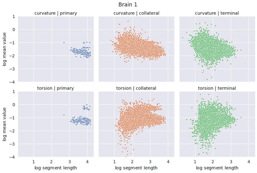
axon geometry, but this feature depends on the definition of start and end points, and cannot capture
an axon’s curvature at a single point.
    In this work, we look at neuron traces through the lens of differential geometry. In particular, we
establish a system of fitting interpolating splines to the neuron traces, and computing their curvature
and torsion properties. To our knowledge, curvature and torsion have never been measured in neuron
traces. We applied this method to cortical projection neuron traces from two mouse brains in the
MouseLight dataset from HHMI Janelia [6]. In both brains, we found different distributions of these
properties between primary, collateral, and terminal axon segments. The code used in this work is
available in our open-source Python package brainlit: http://brainlit.neurodata.io/.
2   Methods
2.1 Spline Fitting First, the neuron traces were split into segments by recursively identifying the
longest root to leaf path (Figure 1a). The first axon segment to be isolated in this way was defined to
be the “primary” segment. Subsequent segments that branched were defined as “collateral” segments,
and those that did not branch were defined to be “terminal” segments (Figure 1b). This classification
approximates the standard morphological definitions of primary, collateral and terminal axon branches.
     Next, a B-spline was fit to each point sequence using scipy’s function splprep [7]. Kunoth
et al. [8] provide an in depth description of B-splines and their applications. Briefly, B-splines are
linear combinations of piecewise polynomials, sometimes called basis functions. The basis functions
are defined by a set of knots, which determine where the polynomial pieces meet, and degree, which
determines the degree of the polynomial pieces. The j ’th basis function for a set of knots ξ and degree
p is recursively defined by (Equation 1.1 in Kunoth et al. [8]):

                                      x − ξj                   ξj+p+1 − x
                    Bj,p,ξ :=                 Bj,p−1,ξ (x) +               Bj+1,p−1,ξ (x)
                                    ξj+p − ξj                ξj+p+1 − ξj+1
                             with
                                (
                                 1, if x ∈ [ξi , ξi+1 ),
                    Bi,0,ξ   :=
                                 0, otherwise.

    Splines are fit to data by solving a constrained optimization problem, where a smoothing term is
minimized while keeping the residual error under a specified value [9]. Here, we constrain the splines
to pass exactly through all points in the original trace. For a sequence of n points, we fit a spline of
degree min{n − 1, 5} which ensures that the splines are thrice continuously differentiable for segments
that are composed of 5 or more points. This method can be applied to any set of points organized in a
tree structure, such as a SWC file.
2.2 Frenet-Serret Parameters An important advantage of B-splines is that their derivatives can be
computed in closed form. In fact, their derivatives are defined in terms of B-splines as shown below in
Theorem 3 from Kunoth et al. [8]:
   Theorem For a continuously differentiable b spline Bj,p,ξ (·) defined by index j , degree p ≥ 1, and
knot sequence ξ , we have:


                              d                       Bj,p−1,ξ (s)   Bj+1,p−1,ξ (s)
                                 Bj,p,ξ (s) = p                    −
                              ds                      ξj+p − ξj      ξj+p+1 − ξj+1

                                                           2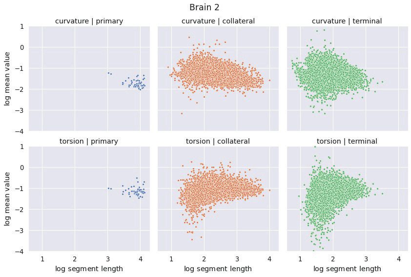
a)    Neuron                             Main branch   Sub-trees                              b)   Segment classification

                                                                                        roots                                 primary
                                                                                                                              collateral
                                                                                                                              terminal

                      find_main_branch()

                                                                           find_main_branch()

Figure 1: a) Illustration of how a neuron trace is split into different segments. This process identifies the longest root to leaf
path (“Main branch”), and separates sub-trees from it. The sub-trees which still have branch points are processed in the same
way until the neuron has been split into segments. By using path length to identify the Main branch, this splitting process
is invariant to rigid transformations of the trace. b) Illustration of how axon segments are classified as primary, collateral, or
terminal. The first segment is defined as primary, and segments that have no sub-trees are defined as terminal. All other
segments are defined as collateral.

    where we assume by convention that fractions with zero denominator have value zero.
    Curvature and torsion can be easily computed because of this property. For a thrice differentiable
curve x(s) ∈ R3 that is parameterized by arc length (i.e. ||ẋ(s)|| = 1 ∀s), one can compute the
curvature (κ) and torsion (τ ) with the following formulas:

                                                κ(s) = ||ẋ(s) × ẍ(s)||
                                                                           ...
                                                        h(ẋ(s) × ẍ(s)), x (s)i
                                                τ (s) =
                                                            ||ẋ(s) × ẍ(s)||2

defined with the standard Euclidean norm ||·||, inner product h·, ·i, and cross product ×. When curvature
vanishes, we define torsion to be zero as well, since the torsion equation becomes undefined.
    Curvature measures how much a curve deviates from being straight, and torsion measures how
much a curve deviates from being planar. Together, these quantities parameterize the Frenet-Serret
formulas of differential geometry. These formulas completely characterize continuously differentiable
curves in three-dimensional Euclidean space, up to rigid motion [10]. Curvature takes non-negative
values, but torsion can be positive or negative where the sign denotes the direction of the torsion in the
right-handed coordinate system. In this work, we are not interested in the direction of the torsion, so
we focused on the torsion magnitude (absolute value).
2.3 Data We applied our methods to a collection of cortical projection neuron axon traces from two
mouse brains in the HHMI Janelia MouseLight dataset [6]. Each reconstruction was reviewed by two
independent annotators. There were 180 traces from brain 1 and 50 traces from brain 2.
    After fitting splines to these traces, curvature and torsion magnitude were sampled uniformly along
the axon segments (details on the spacing is given in Section 3.1). We studied curvature and torsion
magnitude in two ways. First, we studied the autocorrelation of curvature and torsion magnitude along
the axon segments (Section 3.1). Second, we estimated each segment’s average curvature/torsion
magnitude by taking the mean of all points that were sampled on that segment (Section 3.2).
2.4 Statistical Analysis We developed a method for testing for differences in average curvature/torsion
between two different segment classes (primary vs. collateral, collateral vs. terminal, primary vs. ter-
minal). Different neurons represented different samples, and the average curvature/torsion of the two

                                                                 3
segment classes represented the paired measurements.
Define the random variable X as the average curvature/torsion of one segment class and Y as the
average curvature/torsion of another segment class. Further, say X and Y are both real valued. Our
null and alternative hypotheses are as follows:
H0 : Pr[X > Y ] = 0.5
H1 : Pr[X > Y ] 6= 0.5
We tested these hypotheses using the sign test [11]. The test statistic is the number of times that
the data point from one sample is greater than its pair from the other sample. A key advantage of
the sign test is that it does not require parametric distribution assumptions, such as normality of the
data. Also, its null distribution can be computed exactly via the binomial distribution. The two different
parameters (curvature and torsion), and the three different segment class pairs constitute six total tests,
so we applied the Bonferroni correction to α = 0.05 in order to control the family-wise error rate to 0.05.
We conducted one-sided sign tests in all cases.
3 Results
3.1 Autocorrelation of Curvature and Torsion For each axon segment, curvature and torsion mag-
nitude were sampled every 1 µm, then the autocorrelation functions were computed. The autocorrela-
tion functions for all segments of a brain were averaged, and they are shown in Figure 2. These plots
indicate that, on average, the curvature and torsion of axons is correlated between points that are within
5 µm of each other. At 14 µm, autocorrelation for both curvature, and torsion magnitude was less than
0.1 in both brains, so we used this spacing in Section 3.2.
Brain 1 Brain 2
1.0
0.8
Autocorrelation
0.6
0.4 curvature
torsion
0.2
0.0
0 5 10 15 20 25 0 5 10 15 20 25
Lag (μm) Lag (μm)
Figure 2: Autocorrelation of curvature and torsion magnitude averaged across all axon segments. Curvature and torsion were
sampled at every 1 µm along the axon segments. Both curvature and torsion are highly correlated at lag of < 5 µm, but this
correlation drops close to 0 around a lag of 10 µm.
3.2 Axon Segments The distributions of mean curvature and torsion are shown in Figure 3. Our
statistical testing procedure, described in Section 2.4, rejected the null hypothesis in all cases, with all
p-values less than 5 × 10⁻⁴ . The directionality of the one-sided tests were identical in both brains with:
4Figure 3: The distributions of average curvature and average torsion differed between the different segment classes as shown
in these kernel density estimates, using a Gaussian kernel with a standard deviation of 1.2. Segment averages were computed
by sampling the curves at a uniform spacing of 14 µm. One-sided sign tests, testing for differences in average curvature and
torsion, were conducted while controlling the family-wise error rate to 0.05. The tests were significant in all cases and the
directionality of the tests agreed in both brains.
Curvature: Collateral > Terminal > Primary
Torsion: Collateral > Primary > Terminal
Neuron counts for all 36 possible curvature/torsion orderings across classes, and example traces
are shown in the Appendix.
Figure 4 shows the relationships between curvature/torsion and segment length. In order to display
the data on log-log plots, we removed all segments with zero average curvature/torsion. Over 99.9%
of segments that were removed for this reason had only two or three trace points. There appear to be
modest correlations between segment length and curvature/torsion values.
56 Figure 4: The above plots show the relationship between segment length, and mean curvature or torsion in each segment class and brain. Each data point represents a single axon segment, and average curvature and torsion was computed by sampling the segments at a uniform spacing of 14 µm. We removed segments with zero average curvature/torsion in order to plot the data on a log scale. In this data, there appear to be weak negative correlations between segment length and curvature, and a weak positive correlations between segment length torsion.
4 Discussion Our work proposes a model of neuron morphology using continuously differentiable
B-splines. From these curves, it is possible to measure kinematic properties of neuronal processes,
including curvature and torsion. These techniques, along with code to reproduce these results, are
freely available in our open source Python package brainlit: http://brainlit.neurodata.io/.
     We applied these methods to a dataset of 230 projection neuron traces from two different mouse
brains. We found that the autocorrelation functions of both curvature and torsion magnitude drop to 0
at a lag of around 10 µm. Next, we defined segments as either “primary,” “collateral,” or “terminal,” and
found significant differences in the distributions of curvature and torsion between these classes. We also
show what appears to be modest correlations between segment length and average curvature/torsion.
     The statistical analysis approach described in Section 2.4 satisfies two desirable properties. First,
by averaging measurements across segment classes, and pairing the data, we did not have to assume
independence between segments of the same neuron. Assuming independence seemed inappropriate
because, for example, segments that are connected to each other may have correlated geometry. Sec-
ond, it avoided any parametric assumptions of the data, such as assuming normality of curvature/torsion
measurements. A normality assumption seemed inappropriates for several reasons, including the fact
that curvature is nonnegative, and that curvature/torsion was identically 0 for short segments with only
2 trace points.
     Together, these findings suggest that the geometry of primary axon branches is different than that of
higher order branches, such as the segments in terminal arborizations. However, the primary limitation
of our work is that our process of splitting a neuron trace into segments is based on segment length,
and may not exactly partition the neuron into primary, collateral, and terminal branches according to
their standard morphological definitions. Typically, collaterals are defined as branches that split off their
parent branch at sharp angles, and arborize in a different location from other branches [12]. Future
work could include changing our definitions of these classes to more closely reflect morphological
definitions from scientific literature. Also, extending these experiments to neuron trace repositories
such as NeuroMorpho.org would help verify if our findings generalize.
     Previous research has already indicated differences in axon geometry across neuronal cell types.
For example, Stepanyants et al. [13] found higher tortuosity in the axons GABAergic interneurons ver-
sus those of pyramidal cells. Similarly, Portera-Cailliau et al. [14] found Cajal-Retzius cells to be sig-
nificantly more tortuous than Thalamocortical (TC) cells, which is a type of projection neuron. Portera-
Cailliau et al. [14] also offers evidence that, while the primary axon in TC cells travel via a growth cone,
most branching occurs via an interstitial, growth cone independent process. Our work elaborates on
this distinction, suggesting that higher order axon branches have different geometry as well. While
earlier research studied the differences of axonal geometry between neurons, we studied the variation
of axonal geometry within neurons.
     It is also worth noting that this is not the first work to model neuron traces as continuous curves in
R3 . For example, Duncan et al. [15] construct a sophisticated and elegant representation of neurons
that offers several useful properties. First, their representation is invariant to rigid motion and repa-
rameterization. Second, their representation offers a vector space with a shape metric amenable to
clustering and classification. However, their representation is limited to neuron topologies consisting of
a main branch and only first order collaterals. Our B-splines approach does not immediately yield vector
space properties, but can be applied to neurons with higher order branching, and allows for closed form
computation of curvature and torsion. In short, the representation in Duncan et al. [15] is designed for
analysis between neurons, and our representation is designed for analysis within neurons. In the future,
we are interested in bringing the advantages of their work to the open source software community, and

                                                     7
combining it with the advantages of ours.
It is well known that axons are pruned and modified after, and even during, their growth [14]. It is
possible that this process contributes to the different geometry of proximal versus distal axonal seg-
ments. Indeed, Portera-Cailliau et al. [14] mentions the growth of short twisted branches towards the
end of axon development. Future animal experiments could follow-up on this idea, and similar experi-
ments to this one could be applied to other neuron types and other species to see if this is a widespread
phenomenon in neuron morphology.
Conflict of Interest Statement MM own Anatomy Works with the arrangement being managed by
Johns Hopkins University in accordance with its conflict of interest policies. The remaining authors
declare that the research was conducted in the absence of any commercial or financial relationships
that could be construed as a potential conflict of interest.
The funders had no role in study design, data collection and analysis, decision to publish, or prepa-
ration of the manuscript.
Author Contributions MM and DT advised on the theoretical direction of the paper. UM advised on
the data application experiments. JV advised on the presentation of the results. TA and JT designed
the study, implemented the software, and managed the manuscript text/figures. All authors contributed
to manuscript revision.
Funding This work is supported by the National Institutes of Health grants RF1MH121539,
P41EB015909, R01NS086888, U19AG033655 and the National Science Foundation Grant 2014862.
Acknowledgments We thank the MouseLight team at HHMI Janelia for providing us with access to
this data, and answering our questions about it.
Data Availability Statement The datasets analyzed for this study can be found in the Open Neurodata
AWS account: s3://open-neurodata/brainlit/brain1_segments and s3://open-neurodata/brainlit/brain2_
segments.
References
[1] Ruchi Parekh and Giorgio A Ascoli. Neuronal morphology goes digital: a research hub for cellular
and system neuroscience. Neuron, 77(6):1017–1038, 2013.
[2] Antonella Antonini and Michael P Stryker. Rapid remodeling of axonal arbors in the visual cortex.
Science, 260(5115):1819–1821, 1993.
[3] David MacLeod, Julia Dowman, Rachel Hammond, Thomas Leete, Keiichi Inoue, and Asa Abe-
liovich. The familial parkinsonism gene lrrk2 regulates neurite process morphology. Neuron, 52
(4):587–593, 2006.
[4] Giorgio A. Ascoli, Duncan E. Donohue, and Maryam Halavi. Neuromorpho.org: A central resource
for neuronal morphologies. Journal of Neuroscience, 27(35):9247–9251, 2007. ISSN 0270-6474.
doi: 10.1523/JNEUROSCI.2055-07.2007. URL https://www.jneurosci.org/content/27/35/9247.
[5] Holger Heumann and Gabriel Wittum. The tree-edit-distance, a measure for quantifying neuronal
morphology. Neuroinformatics, 7(3):179–190, 2009.
[6] Johan Winnubst, Erhan Bas, Tiago A Ferreira, Zhuhao Wu, Michael N Economo, Patrick Edson,
Ben J Arthur, Christopher Bruns, Konrad Rokicki, David Schauder, et al. Reconstruction of 1,000
projection neurons reveals new cell types and organization of long-range connectivity in the mouse
brain. Cell, 179(1):268–281, 2019.
8[7] Pauli Virtanen, Ralf Gommers, Travis E. Oliphant, Matt Haberland, Tyler Reddy, David Courna-
peau, Evgeni Burovski, Pearu Peterson, Warren Weckesser, Jonathan Bright, Stéfan J. van der
Walt, Matthew Brett, Joshua Wilson, K. Jarrod Millman, Nikolay Mayorov, Andrew R. J. Nelson,
Eric Jones, Robert Kern, Eric Larson, C J Carey, İlhan Polat, Yu Feng, Eric W. Moore, Jake Vander-
Plas, Denis Laxalde, Josef Perktold, Robert Cimrman, Ian Henriksen, E. A. Quintero, Charles R.
Harris, Anne M. Archibald, Antônio H. Ribeiro, Fabian Pedregosa, Paul van Mulbregt, and SciPy
1.0 Contributors. SciPy 1.0: Fundamental Algorithms for Scientific Computing in Python. Nature
Methods, 17:261–272, 2020. doi: 10.1038/s41592-019-0686-2.
[8] Angela Kunoth, Tom Lyche, Giancarlo Sangalli, and Stefano Serra-Capizzano. Splines and PDEs:
From approximation theory to numerical linear algebra. Springer, 2018.
[9] Paul Dierckx. Algorithms for smoothing data with periodic and parametric splines. Computer
Graphics and Image Processing, 20(2):171–184, 1982.
[10] Ulf Grenander, Michael I Miller, Michael Miller, et al. Pattern theory: from representation to
inference. Oxford university press, 2007.
[11] Markus Neuhauser. Nonparametric statistical tests: A computational approach. CRC Press, 2011.
[12] Kathleen S Rockland. Collateral branching of long-distance cortical projections in monkey. Journal
of Comparative Neurology, 521(18):4112–4123, 2013.
[13] Armen Stepanyants, Gábor Tamás, and Dmitri B Chklovskii. Class-specific features of neuronal
wiring. Neuron, 43(2):251–259, 2004. ISSN 0896-6273. doi: https://doi.org/10.1016/j.neuron.
2004.06.013. URL https://www.sciencedirect.com/science/article/pii/S0896627304003629.
[14] Carlos Portera-Cailliau, Robby M Weimer, Vincenzo De Paola, Pico Caroni, and Karel Svoboda.
Diverse modes of axon elaboration in the developing neocortex. PLoS Biol, 3(8):e272, 2005.
[15] Adam Duncan, Eric Klassen, Anuj Srivastava, et al. Statistical shape analysis of simplified neu-
ronal trees. Annals of Applied Statistics, 12(3):1385–1421, 2018.
9Appendix A. Supplementary Figures.
Brain 1 curvature (α = 0.24) Brain 1 torsion (α = 0.39)
1.75
1.50
1.25
1.00
density
0.75
0.50
0.25
0.00
Magnitude
Brain 2 curvature (α = 0.21) Brain 2 torsion (α = 0.35) non-zero
1.75 zero
1.50
1.25
1.00
density
0.75
0.50
0.25
0.00
0 1 2 3 4 0 1 2 3 4
log segment length log segment length
Figure 5: Segments with zero curvature or torsion were typically the shortest of all the segments. In almost all cases,
segments had zero curvature/torsion because the segment was only composed of two or three trace points. α indicates the
fraction of segments that had zero curvature/torsion in each brain.
10Torsion
p>c>t p>t>c c>p>t c>t>p t>p>c t>c>p
p>c>t 0 0 0 0 0 0
p>t>c 0 0 0 0 0 0
c>p>t 5 0 8 0 0 0
Curvature
c>t>p 19 0 90 11 0 0
t>p>c 1 0 0 0 0 0
t>c>p 18 0 24 4 0 0
Table 1: For each neuron, average curvature and torsion was computed for all three segment classes (p=primary, c=collateral,
t=terminal) and compared between classes. This table shows the neuron counts for brain 1 for all 36 possible orderings of
curvature/torsion. The most common ordering was collateral > terminal > primary for curvature and collateral > primary >
terminal for torsion. For example traces see Figure 6.
Torsion
p>c>t p>t>c c>p>t c>t>p t>p>c t>c>p
p>c>t 2 0 0 0 0 0
p>t>c 0 0 0 0 0 0
c>p>t 0 0 1 0 0 0
Curvature
c>t>p 11 0 30 1 0 0
t>p>c 0 0 0 0 0 0
t>c>p 0 0 3 2 0 0
Table 2: Same data as in Table 1 except for brain 2.
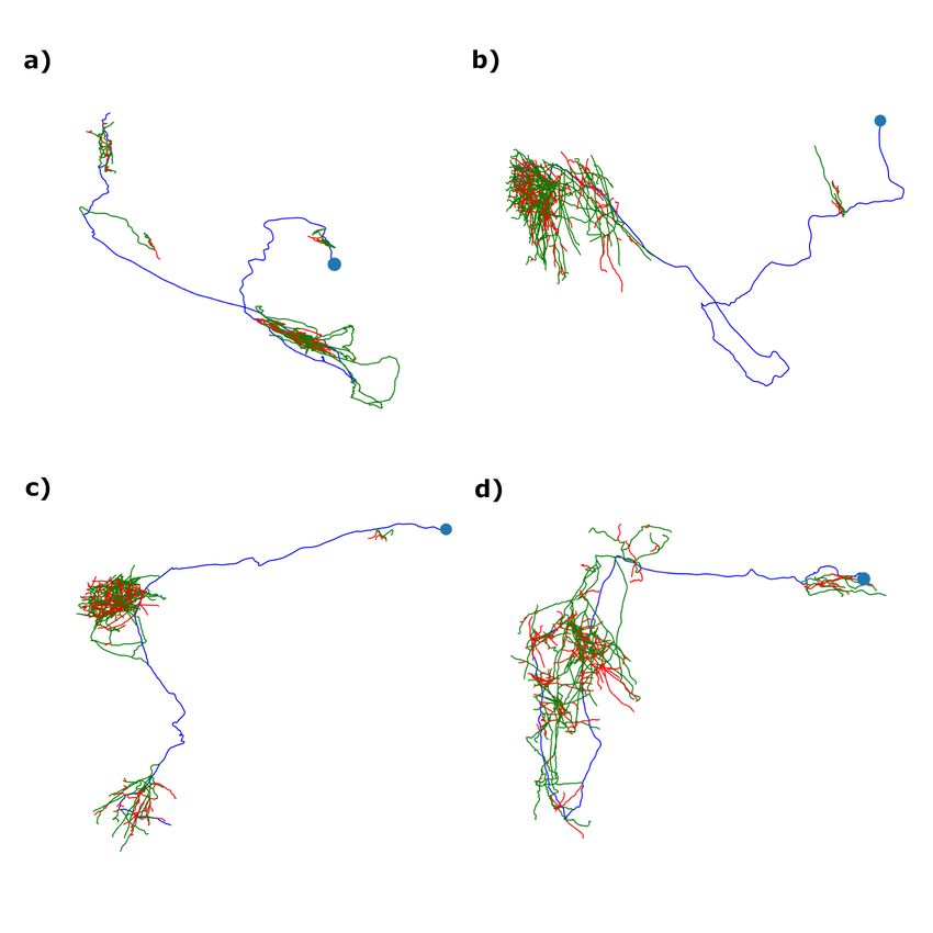
11Figure 6: Example neuron traces composed of somas (blue points), primary segments (blue lines), collateral segments
(green lines), and terminal segments (red lines). a,c) Examples of neurons that exhibit the most common class orderings of
curvature/torsion (collateral > terminal > primary for curvature and collateral > primary > terminal for torsion - see Tables 1,
2). b,d) Examples of neurons that do not exhibit the most common class orderings of curvature/torsion. a,b) are from brain 1
and c,d) are from brain 2.
12You can also read