Federated Hyperparameter Tuning: Challenges, Baselines, and Connections to Weight-Sharing
←
→
Page content transcription
If your browser does not render page correctly, please read the page content below
Federated Hyperparameter Tuning: Challenges,
                                              Baselines, and Connections to Weight-Sharing

                                                      Mikhail Khodak, Renbo Tu, Tian Li                           Liam Li
                                                          Carnegie Mellon University                           Determined AI
                                                      {khodak,renbo,tianli}@cmu.edu                           me@liamcli.com
arXiv:2106.04502v1 [cs.LG] 8 Jun 2021

                                             Maria-Florina Balcan, Virginia Smith                       Ameet Talwalkar
                                                  Carnegie Mellon University                Carnegie Mellon University & Determined AI
                                            ninamf@cs.cmu.edu,smithv@cmu.edu                          talwalkar@cmu.edu

                                                                                      Abstract
                                                 Tuning hyperparameters is a crucial but arduous part of the machine learning
                                                 pipeline. Hyperparameter optimization is even more challenging in federated learn-
                                                 ing, where models are learned over a distributed network of heterogeneous devices;
                                                 here, the need to keep data on device and perform local training makes it difficult to
                                                 efficiently train and evaluate configurations. In this work, we investigate the prob-
                                                 lem of federated hyperparameter tuning. We first identify key challenges and show
                                                 how standard approaches may be adapted to form baselines for the federated setting.
                                                 Then, by making a novel connection to the neural architecture search technique
                                                 of weight-sharing, we introduce a new method, FedEx, to accelerate federated
                                                 hyperparameter tuning that is applicable to widely-used federated optimization
                                                 methods such as FedAvg and recent variants. Theoretically, we show that a FedEx
                                                 variant correctly tunes the on-device learning rate in the setting of online convex
                                                 optimization across devices. Empirically, we show that FedEx can outperform
                                                 natural baselines for federated hyperparameter tuning by several percentage points
                                                 on the Shakespeare, FEMNIST, and CIFAR-10 benchmarks—obtaining higher
                                                 accuracy using the same training budget.

                                        1    Introduction
                                        Federated learning (FL) is a popular distributed computational setting where training is performed
                                        locally or privately [30, 36] and where hyperparameter tuning has been identified as a critical
                                        problem [18]. Although general hyperparameter optimization has been the subject of intense study [4,
                                        16, 26], several unique aspects of the federated setting make tuning hyperparameters especially
                                        challenging. However, to the best of our knowledge there has been no dedicated study on the specific
                                        challenges and solutions in federated hyperparameter tuning. In this work, we first formalize the
                                        problem of hyperparameter optimization in FL, introducing the following three key challenges:
                                        1. Federated validation data: In federated networks, as the validation data is split across devices,
                                           the entire dataset is not available at any one time; instead a central server is given access to
                                           some number of devices at each communication round, for one or at most a few runs of local
                                           training and validation. Thus, because the standard measure of complexity in FL is the number of
                                           communication rounds, computing validation metrics exactly dramatically increases the cost.
                                        2. Extreme resource limitations: FL applications often involve training using devices with very
                                           limited computational and communication capabilities. Furthermore, many require the use of
                                           privacy techniques such as differential privacy that limit the number times user data can be accessed.
                                           Thus we cannot depend on being able to run many different configurations to completion.

                                        Preprint. Under review.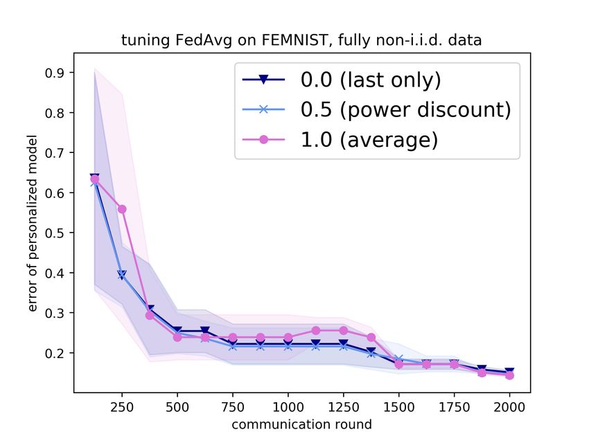
Figure 1: FedEx can be applied to any local training-based FL method, e.g. FedAvg, by interleaving
standard updates to model weights (computed by aggregating results of local training) with exponen-
tiated gradient updates to hyperparameters (computed by aggregating results of local validation).

3. Evaluating personalization: Finally, even with non-federated data, applying common hyperpa-
   rameter optimization methods to standard personalized FL approaches (such as finetuning) can be
   costly because evaluation may require performing many additional training steps locally.
With these challenges in mind, we propose reasonable baselines for federated hyperparameter tuning
by showing how to adapt standard non-federated algorithms. We further study the challenge of noisy
validation signal due to federation, and show that simple state-estimation-based fixes do not help.
Our formalization and analysis of this problem leads us to develop FedEx, a method that exploits
a novel connection between hyperparameter tuning in FL and the weight-sharing technique widely
used in neural architecture search (NAS) [5, 34, 40]. In particular, we observe that weight-sharing
is a natural way of addressing the three challenges above for federated hyperparameter tuning, as
it incorporates noisy validation signal, simultaneously tunes and trains the model, and evaluates
personalization as part of training rather than as a costly separate step. Although standard weight-
sharing only handles architectural hyperparameters such as the choice of layer or activation, and not
critical settings such as those of local stochastic gradient descent (SGD), we develop a formulation
that allows us to tune most of these as well via the relationship between local-training and fine-tuning-
based personalization. This make FedEx a general hyperparameter tuning algorithm applicable to
many local training-based FL methods, e.g. FedAvg [36], FedProx [31], and SCAFFOLD [19].
In Section 4, we next conduct a theoretical study of FedEx in a simple setting: tuning the client
step-size. Using the ARUBA framework for analyzing meta-learning [20], we show that a variant
of FedEx correctly tunes the on-device step-size to minimize client-averaged regret by adapting to
the intrinsic similarity between client data. We improve the convergence rate compared to some past
meta-learning theory [20, 25] while not depending on knowing the (usually unknown) task-similarity.
Finally, in Section 5, we instantiate our baselines and FedEx to tune hyperparameters of FedAvg,
FedProx, and Reptile, evaluating on three standard FL benchmarks: Shakespeare, FEMNIST, and
CIFAR-10 [6, 36]. While our baselines already obtain performance similar to past hand-tuning,
FedEx further surpasses them in most settings examined, including by 2-3% on Shakespeare.

Related Work To the best of our knowledge, we are the first to systematically analyze the formu-
lation and challenges of hyperparameter optimization in the federated setting. Several papers have
explored limited aspects of hyperparameter tuning in FL [8, 23, 38], focusing on a small number of
hyperparameters (e.g. the step-size and sometimes one or two more) in less general settings (studying
small-scale problems or assuming server-side validation data). In contrast our methods are able to
tune a wide range of hyperparameters in realistic federated networks. Some papers also discussed the
challenges of finding good configurations while studying other aspects of federated training [41]. We
argue that it is critical to properly address the challenges of federated hyperparameter optimization in
practical settings, as we discuss in detail in Section 2.
Methodologically, our approach draws on the fact that local training-based methods such as FedAvg
can be viewed as optimizing a surrogate objective for personalization [20], and more broadly leverages
the similarity of the personalized FL setup and initialization-based meta-learning [7, 11, 17, 25].
While FedEx’s formulation and guarantees use this relationship, the method itself is general-purpose
and applicable to federated training of a single global model. Many recent papers address FL
personalization more directly [14, 29, 35, 44, 47]. This connection and our use of NAS techniques
also makes research connecting NAS and meta-learning relevant [10, 33], but unlike these methods we
focus on tuning non-architectural parameters. In fact, we believe our work is the first to apply weight-
sharing to regular hyperparameter search. Furthermore, meta-learning does not have the data-access
and computational restrictions of FL, where such methods using the DARTS mixture relaxation [34]

                                                   2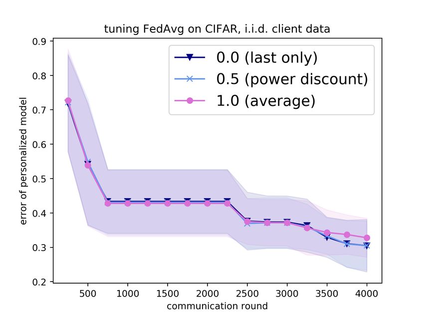
are less practical. Instead, FedEx employs the lower-overhead stochastic relaxation [9, 28], and its
exponentiated update is similar to the recently proposed GAEA approach for NAS [27]. Running NAS
itself in federated settings has also been studied [13, 15, 46]; while our focus is on non-architectural
hyperparameters, in-principle our algorithms can also be used for federated NAS.

2       Federated Hyperparameter Optimization
In this section we formalize the problem of hyperparameter optimization for FL and discuss the con-
nection of its personalized variant to meta-learning. We also review FedAvg [36], a common federated
optimization method, and present a reasonable baseline approach for tuning its hyperparameters.

Global and Personalized FL In FL we are concerned with optimizing over a network of heteroge-
neous clients i = 1, . . . , n, each with training, validation, and testing sets Ti , Vi , and Ei , respectively.
We use LS (w) to denote the average loss over a dataset S of some w-parameterized ML model, for
w ∈ Rd some real vector. For hyperparameter optimization, we assume a class of algorithms Alga
hyperparameterized by a ∈ A that use federated access to training sets Ti to output some element of
Rd . Here by “federated access" we mean that each iteration corresponds to a communication round at
which Alga has access to a batch of B clients1 that can do local training and validation.
Specifically, we assume Alga can be described by two subroutines with hyperparameters encoded
by b ∈ B and c ∈ C, so that a = (b, c) and A = B × C. Here c encodes settings of a local training
algorithm SGDc that take a training set S and initialization w ∈ Rd as input and outputs a model
SGDc (S, w) ∈ Rd , while b sets those of an aggregation Aggb that takes the initialization w and
outputs of SGDc as input and returns a model parameter. For example, in standard FedAvg, SGDc is
T steps of gradient descent with step-size η and Aggb takes a weighted average of the outputs of
SGDc across clients; here c = (η, T ) and b = (). As detailed in the appendix, many FL methods
can be decomposed this way, including well-known ones such as FedAvg [36], FedProx [31],
SCAFFOLD [19], and Reptile [39] as well as more recent methods [1, 2, 29]. Our analysis and our
proposed FedEx algorithm will thus apply to all of them, up to an assumption detailed next.
Starting from this decomposition, the global hyperparameter optimization problem can be written as
                                       Xn
                               min         |Vi |LVi (Alga ({Tj }nj=1 ))                         (1)
                                      a∈A
                                               i=1

In many cases we are also interested in obtaining a device-specific local model, where we take
a model trained on all clients and finetune it on each individual client before evaluating. A key
assumption we make is that the finetuning algorithm will be the same as the local training algorithm
SGDc used by Alga . This assumption can be justified by recent work in meta-learning that shows that
algorithms that aggregate the outputs of local SGD can be viewed as optimizing for personalization
using local SGD [20]. Then, in the personalized setting, the tuning objective becomes
                                     Xn
                           min           |Vi |LVi (SGDc (Ti , Alga ({Tj }nj=1 ))                  (2)
                              a=(b,c)∈A
                                            i=1

Our approach will focus on the setting where the hyperparameters c of local training make up a
significant portion of all hyperparameters a = (b, c); by considering the personalization objective we
will be able to treat such hyperparameters as architectural and thus apply weight-sharing.

Tuning FL Methods: Challenges and Baselines In the non-federated setting, the objective (1) is
amenable to regular hyperparameter optimization methods; for example, a random search approach
would repeatedly sample a setting a from some distribution over A, run Alga to completion, and eval-
uate the objective, saving the best setting and output [4]. With a reasonable distribution and enough
samples this is guaranteed to converge and can be accelerated using early stopping methods [26], in
which Alga is not always run to completion if the desired objective is poor at intermediate stages,
or by adapting the sampling distribution using the results of previous objective evaluations [45]. As
mentioned in the introduction, applying such methods to FL is inherently challenging due to
1. Federated validation data: Separating data across devices means we cannot immediately get
   a good estimate of the model’s validation performance, as we only have access to a possibly
1
    For simplicity the number of clients per round is fixed, but all methods can be easily generalized to varying B.

                                                          3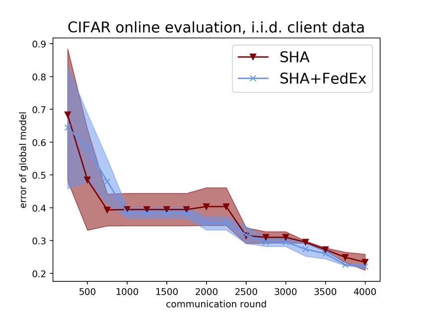
Algorithm 1: Successive halving algorithm (SHA) ap-
plied to personalized FL. For the non-personalized ob-
jective (1), replace LVti (wi ) by LVti (wa ). For random
search (RS) with N samples, set η = N and R = 1.
Input: distribution D over hyperparameters A,
elimination rate η ∈ N, elimination rounds
τ0 = 0, τ1 , . . . , τR
R
sample set of η R hyperparameters H ∼ D[η ]
initialize a model wa ∈ Rd for each a ∈ H
for elimination round r ∈ [R] do
for setting a = (b, c) ∈ H do
for comm. round t = τr−1 + 1, . . . , τr do
for client i = 1, . . . , B do
send wa , c to client
wi ← SGDc (Tti , wa )
send wi , LVti (wi ) to server
Figure 2: Tuning FL with SHA but mak-
wa ← Aggb (wa , {wi }B i=1 ) P ing elimination decisions based on vali-
PB B
sa ← i=1 |Vti |LVti (wi )/ i=1 |Vti | dation estimates using different discount
factors. On both FEMNIST (top) and CI-
H ← {a ∈ H : sa ≤ η1 -quantile({sa : a ∈ H})} FAR (bottom) using more of the validation
Output: remaining a ∈ H and associated model wa data does not improve upon just using the
most recent round’s validation error.
small batch of devices at a time. This means that decisions such as which models to flag for early
stopping will be noisy and may not fully incorporate all the available validation signal.
2. Extreme resource limitations: As FL algorithms can take a very long time to run in-practice due
to the weakness and spotty availability of devices, we often cannot afford to conduct many training
runs to evaluate different configurations. This issue is made more salient in cases where we use of
privacy techniques that only allow a limited number of accesses to the data of any individual user.
3. Evaluating personalization: While personalization is important in FL due to client heterogeneity,
checking the performance of the current model on the personalization objective (2) is computation-
ally intensive because computing may require running local training multiple times. In particular,
while regular validation losses require computing one forward pass per data point, personalized
losses require several forward-backward passes, making it many times more expensive if this loss
is needed to make a tuning decision such as eliminating a configuration from consideration.
Despite these challenges, we can still devise sensible baselines for tuning hyperparameters in FL,
most straightforward of which is to use a regular hyperparameter method but use validation data
from a single round as a noisy surrogate for the full validation objective. Specifically, one can use
random search (RS)—repeatedly evaluate random configurations—and a simple generalization called
successive halving (SHA), in which we sample a set of configurations and partially run all of them
for some number of communication rounds before eliminating all but the best η1 fraction, repeating
until only one configuration remains. Note both are equivalent to a “bracket” in Hyperband [26].
As shown in Section 5, SHA performs reasonably well on the benchmarks we consider. However,
by using validation data from one round it may make noisy elimination decisions, early-stopping
potentially good configurations because of a difficult set of clients on a particular round. Here the
problem is one of insufficient utilization of the validation data to estimate model performance. A
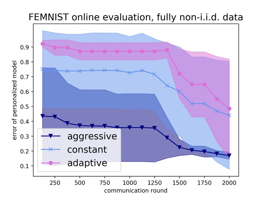
reasonable approach to use more is to try some type of state-estimation: using the performance from
previous rounds to improve the noisy measurement of the current one. For example, instead of using
only the most recent round for elimination decisions we can use a weighted sum of the performances
at all past rounds. To investigate this, we study a power decay weighting, where a round is discounted
by some constant factor for each time step it is in the past. We consider factors 0.0 (taking the most
recent performance only, as before), 0.5, and 1.0 (taking the average). However, in Figure 2 we show
that incorporating more validation data this way does not significantly affect results.
Thus we may need a better algorithm to use more of the validation signal, most of which is discarded
by using the most recent round’s performance. We next propose FedEx, a new method that does so
4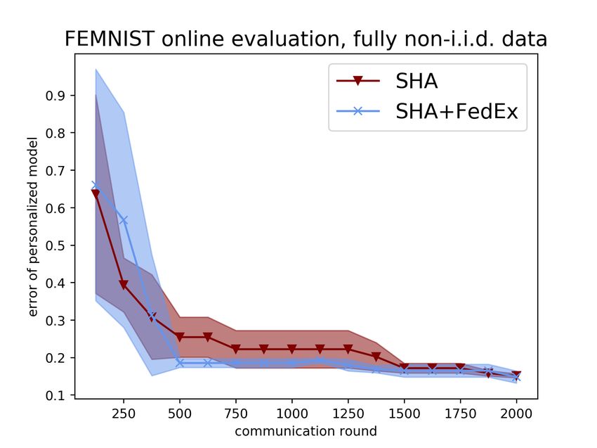
by using validation on each round to update a client hyperparameters distribution used to sample
configurations to send to devices. Thus it alleviates issue (1) above by updating at each step, not
waiting for an elimination round as in RS or SHA. By simultaneously training the model and tuning
(client) hyperparameters, it also moves towards a fully single-shot procedure in which we only train
once (we must still run multiple times due to server hyperparameters), which would solve issue (2).
Finally, FedEx addresses issue (3) by using local training to both update the model and to estimate
personalized validation loss, thus not spending extra computation on this more expensive objective.

3   Weight-Sharing for Federated Learning
We now present FedEx, a way to tune local FL hyperparameters. This section contains the general
algorithm and its connection to weight-sharing; we instantiate it on several FL methods in Section 5.

Weight-Sharing for Architecture Search We first review the weight-sharing approach in NAS,
which for a set C of network configurations is often posed as the bilevel optimization
                          min Lvalid (w, c) s.t. w ∈ arg min Ltrain (u, c)                           (3)
                          c∈C                                  u∈Rd

where Ltrain , Lvalid evaluate a single configuration with the given weights. If, as in NAS, all hyperpa-
rameters are architectural, then they are effectively themselves trainable model parameters [27], so
we could instead consider solving the following “single-level" empirical risk minimization (ERM):
                      min       L(w, c)      =         min   Ltrain (w, c) + Lvalid (w, c)           (4)
                    c∈C,w∈Rd                       c∈C,∈Rd

Solving this instead of the bilevel problem (3) has been proposed in several recent papers [24, 27].
Early approaches to solving either formulation of NAS were costly due to the need for full or partial
training of many architectures in a very large search space. The weight-sharing paradigm [40] reduces
the problem to that of training a single architecture, a “supernet" containing all architectures in the
search space C. A straightforward way of constructing a supernet is via a “stochastic relaxation"
where the loss is an expectation w.r.t. sampling c from some distribution over C [9]. Then the shared
weights can be updated using SGD by first sampling an architecture c and using an unbiased estimate
of ∇w L(w, c) to update w. The distribution over C may itself be adapted or stay fixed. We focus on
the former case, adapting some θ-parameterized distribution Dθ ; this yields the objective
                                            min        Ec∼Dθ L(w, c)                                 (5)
                                          θ∈Θ,w∈Rd

Since architectural hyperparameters are often discrete decisions, e.g. a choice of which of a fixed
number of operations to use, a natural choice of Dθ is as a product of categorical distributions over
simplices. In this case, any discretization of an optimum θ of the relaxed objective (5) whose support
is in the support of θ will be an optimum of the original objective (4). A natural update scheme
here is exponentiated gradient [22], where each successive θ is proportional to θ exp(−η ∇),       ˜
η is a step-size, and ∇˜ an unbiased estimate of ∇θ Ec∼D L(w, c) that can be computed using the
                                                            θ
re-parameterization trick [42]. By alternating this exponentiated update with the standard SGD update
to w discussed earlier we obtain a simple block-stochastic minimization scheme that is guaranteed to
converge, under certain conditions, to the ERM objective, and also performs well in practice [27].

The FedEx Method To obtain FedEx from weight-sharing we restrict to the case of tuning only
the hyperparameters c of local training SGDc . We can then replace the personalized objective (2) by
                                           X n
                                  min           |Vi |LVi (SGDc (Ti , w))                          (6)
                                 c∈C,w∈Rd
                                                 i=1
                                      d
Note Alga outputs an element of R , so this new objective is upper-bounded by the original (2). It is
also in the form of the weight-sharing objective (4), so we can apply a NAS-like stochastic relaxation:
                                            n
                                            X
                                min               |Vi |Ec∈Dθ LVi (SGDc (Ti , w))                     (7)
                            θ∈Θ,w∈Rd
                                            i=1
Unlike in NAS, FL hyperparameters such as the learning rate are not extreme points of a simplex and
so it is less clear what parameterized distribution Dθ to use. Nevertheless, we find that by crudely

                                                        5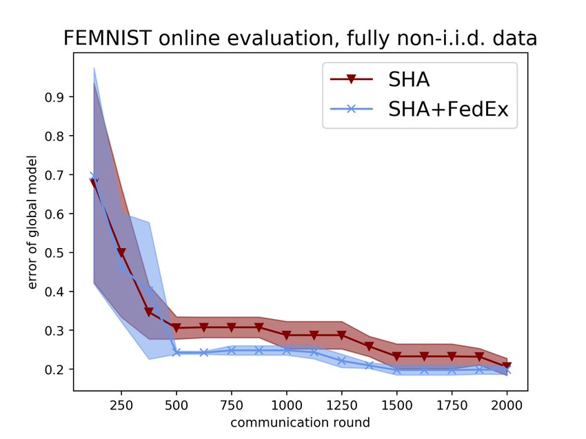
Algorithm 2: FedEx
Input: configurations c1 , . . . , ck ∈ C, setting b for
         Aggb , schemes for setting step-size ηt and
         baseline λt , total number of steps τ ≥ 1
initialize θ1 = 1k /k and shared weights w1 ∈ Rd
for comm. round t = 1, . . . , τ do
     for client i = 1, . . . , B do
         send wt , θt to client
         sample cti ∼ Dθt
         wti ← SGDcti (Tti , wt )                          Figure 3: Comparison of the range of perfor-
         send wti , cti , LVti (wti ) to server            mance values attained using different pertur-
     wt+1 ←    Agg (w, {wti }B
             PB b                 i=1 )
                                                           bation settings. Although the range is much
      ˜j ←     i=1 |Vti |(LVti (wti )−λt )1cti =cj         smaller for  = 0.1 than for  = 1.0 (the lat-
     ∇               θt[j]
                            PB
                                   |Vti |
                                                   ∀j      ter is the entire space), it still covers a large
                             i=1

   θt+1 ← θt exp(−ηt ∇)  ˜                                 (roughly 10-20%) range of different perfor-
   θt+1 ← θt+1 /kθt+1 k1                                   mance levels on both FEMNIST (left) and
Output: model w, hyperparameter distribution θ             CIFAR (right).

imposing a categorical distribution over k > 1 random samples from some distribution (e.g. uniform)
over C and updating θ using exponentiated gradient over the resulting k-simplex works well. We
alternate this with updating w ∈ Rd , which in a NAS algorithm involves an SGD update using
an unbiased estimate of the gradient at the current w and θ. Following the meta-learning method
Reptile [39], we can view the other sub-routine Aggb of Alga that aggregates the outputs of local
training as performing an update using a gradient surrogate of the personalization objective [20].
We call this alternating method for solving (7) FedEx and describe it for a general Alga consisting
of sub-routines Aggb and SGDc in Algorithm 2; recall from Section 2 that many FL methods can
be decomposed this way, so our approach is widely applicable. FedEx has a minimal overhead,
consisting only of the last four lines of the outer loop updating θ. Thus, as with weight-sharing,
FedEx can be viewed as reducing the complexity of tuning local hyperparameters to that of training a
single model. Each update to θ requires a step-size ηt and an approximation ∇ ˜ of the gradient w.r.t. θ;
                                     ˜ j of each gradient entry via the reparameterization trick, whose
for the latter we obtain an estimate ∇
variance we reduce by subtracting a baseline λt . How we set ηt and λt is detailed in the Appendix.

Wrapping FedEx We can view FedEx as an algorithm of the form tuned by Algorithm 1 that
implements federated training of a supernet parameter (w, θ), with the local training routine SGD
including a step for sampling c ∼ Dθ and the server aggregation routine including an exponentiated
update of θ. Thus we can wrap FedEx in Algorithm 1, which we find useful for a variety of reasons:
• The wrapper can tune the settings of b for the aggregation step Aggb , which FedEx cannot.
• FedEx itself has a few hyperparameters, e.g. how to set the baseline λt , which can be tuned.
• By running multiple seeds and potentially using early stopping, we can run FedEx using more
  aggressive steps-sizes and the wrapper will discard cases where this leads to poor results.
• We can directly compare FedEx to a regular hyperparameter optimization scheme run over the
  original algorithm, e.g. FedAvg, by using the same scheme to both wrap FedEx and tune FedAvg.
• Using the wrapper allows us to determine the configurations c1 , . . . , ck given to Algorithm 2 using
  a local perturbation scheme (detailed next) while still exploring the entire hyperparameter space.

Local Perturbation It remains to specify how to select the configurations c1 , . . . , ck ∈ C to pass to
Algorithm 2. While the simplest approach is to draw from Unif k (C), we find that this leads to unstable
behavior if the configurations are too distinct from each other. To interpolate between sampling
ci independently and setting them to be identical (which would just be equivalent to the baseline
algorithm), we use a simple local perturbation method in which c1 is sampled from Unif(C) and
c2 , . . . , ck are sampled uniformly from a local neighborhood of C. For continuous hyperparameters
(e.g. step-size, dropout) drawn from an interval [a, b] ⊂ R the local neighborhood is [c ± (b − a)ε] for
some ε ≥ 0, i.e. a scaled ε-ball; for discrete hyperparameters (e.g. batch-size, epochs) drawn from a
set {a, . . . , b} ⊂ Z, the local neighborhood is similarly {c − b(b − a)εc, . . . , c + d(b − a)εe}; in our

                                                      6
experiments we set ε = 0.1, which works well, but run ablation studies varying these values in the
appendix showing that a wide range of them leads to improvement. Note that while local perturbation
does limit the size of the search space explored by each instance of FedEx, as shown in Figure 3 the
difference in performance between different configurations in the same ball is still substantial.
Limitations of FedEx While FedEx is applicable to many important FL algorithms, those that
cannot be decomposed into local fine-tuning and aggregation should instead be tuned by one of our
baselines, e.g. SHA. FedEx is also limited in that it is forced to rely on such algorithms as wrappers
for tuning its own hyperparameters and certain FL hyperparameters such as server learning rate.
4 Theoretical Analysis for Tuning the Step-Size in an Online Setting
As noted in Section 3, FedEx can be viewed as alternating minimization, with a gradient step on a
surrogate personalization loss and an exponentiated gradient update of the configuration distribution
θ. We make this formal and prove guarantees for a simple variant of FedEx in the setting where
the server has one client per round, to which the server sends an initialization to solve an online
convex optimization (OCO) problem using online gradient descent (OGD) on a sequence of m
adversarial convex losses (i.e. one SGD epoch in the stochastic case). Note we use “client” and “task”
interchangeably, as the goal is a meta-learning (personalization) result. The performance measure
here is task-averaged regret, which takes the average over τ clients of the regret they incur on its loss:
τ m
1 XX
R̄τ = `t,i (wt,i ) − `t,i (wt∗ ) (8)
τ t=1 i=1
Here `t,i is the ith loss of client t, wt,i the parameter
Pm chosen on its ith round from a compact
parameter space W, and wt∗ ∈ arg minw∈W i=1 `t,i (w) the task optimum. In this setting, the
Average Regret-Upper-Bound Analysis (ARUBA) framework [20] can be used to show guarantees
for a Reptile (i.e. FedEx with a server step-size) variant in which at each round the initialization
is updated as wt+1 ← (1 − αt )wt + αt wt∗ for server step-size αt = 1/t. Observe that the only
difference between this update and FedEx’s is that the task-t optimum wt∗ is used rather than the last
iterate of OGD on that task. Specifically they bound task-averaged regret by
τ
√
1 1X
R̄τ ≤ Õ √ + V m for V 2
= min kw − wt∗ k22 (9)
4
τ w∈W τ
t=1
Here V —the average deviation of the optimal actions wt∗ across tasks—is a measure of task-similarity:
V is small when the tasks (clients) have similar data and thus can be solved by similar parameters in W
but large when their data is different and so the optimum parameters to use are very different. Thus the
bound in (9) shows that as the√ server (meta-learning) sees more and more clients (tasks), their regret
on each decays with rate 1/ 4 τ to depend only on the task-similarity, which is hopefully small if the
client data is similar enough that transfer √ V
diam(W). Since
learning makes sense, in particular if √
single-task regret has lower bound Ω(D m), achieving asymptotic regret V m thus demonstrates
successful learning of a useful initialization in W that can be used for personalization. Note that such
bounds can also be converted to obtain guarantees in the statistical meta-learning setting as well [20].
A drawback of past results using the ARUBA framework is that they either assume the task-similarity
V is known in order to set the client step-size [25] or they employ an OCO method to learn the local
step-size that cannot be applied to other potential algorithmic hyperparameters [20]. In contrast, we
prove results for using bandit exponentiated gradient to tune the client step-size, which is precisely
the FedEx update. In particular, Theorem 4.1 shws that by using a discretization of potential client
step-sizes as the configurations in Algorithms 2 we can obtain the following task-averaged regret:
Theorem 4.1. Let W ⊂ Rd be convex and compact with diameter D = diam(W) and let `t,i be
a sequence of mτ b-bounded convex losses—m for each of τ tasks—with Lipschitz constant ≤ G.
We assume that the adversary is oblivious within-task. Suppose we run Algorithm 2 with B = 1,
configurations cj = GjD √ for each j = 1, . . . , k determining the local step-size of single-epoch SGD
mP
∗ m
(OGD), wti = wtq , regret i=1 `t,i (wt,i )−`t,i (wt ) used in place of LVti (wti ), and λt = 0 ∀ t ∈ [τ ].
log k 3
1 DG ∗ ∗
p τ
Then if ηt = mb kτ ∀ t ∈ [τ ], k = b 2m , and Aggb (w, wt ) = (1 − αt )w + αt wt for
2
αt = 1/t ∀ t ∈ [τ ] we have (taking expectations over sampling from Dθt )
p √
ER̄τ ≤ Õ 3 m/τ + V m (10)
7Table 1: Final test error obtained when tuning using a standard hyperparameter tuning algorithm
(SHA or RS) alone, or when using it for server (aggregation) hyperparameters while FedEx tunes
client (on-device training) hyperparameters. The target model is the one used to compute on-device
validation error by the wrapper method, as well as the one used to compute test error after tuning.
Note that this table reports the final error results corresponding to the online evaluations reported in
Figure 4, which measure performance as more of the computational budget is expended.
Wrapper Target Tuning Shakespeare FEMNIST CIFAR-10
method model method i.i.d. non-i.i.d. i.i.d. non-i.i.d. i.i.d.
RS (server & client) 54.89 ± 7.04 55.90 ± 8.72 22.36 ± 2.76 22.55 ± 2.58 36.09 ± 15.03
global
Random + FedEx (client) 55.72 ± 10.84 61.34 ± 16.11 17.62 ± 0.47 19.75 ± 0.23 30.59 ± 1.49
Search person- RS (server & client) 56.26 ± 6.23 57.14 ± 6.54 16.54 ± 1.47 17.45 ± 1.45 42.78 ± 16.30
(RS) alized + FedEx (client) 57.75 ± 11.83 61.20 ± 15.87 18.53 ± 1.89 14.52 ± 1.09 42.07 ± 10.70
SHA (server & client) 48.99 ± 3.23 48.86 ± 3.13 18.77 ± 1.89 20.56 ± 2.17 23.36 ± 2.42
global
Successive + FedEx (client) 45.19 ± 1.85 46.86 ± 3.42 19.75 ± 0.19 19.82 ± 1.18 22.05 ± 0.39
Halving person- SHA (server & client) 48.89 ± 3.22 50.65 ± 2.47 14.38 ± 0.52 15.09 ± 0.53 30.46 ± 7.62
(SHA) alized + FedEx (client) 46.86 ± 3.00 47.02 ± 4.40 14.73 ± 0.69 14.77 ± 1.61 22.43 ± 2.87
The proof of this result, given in the supplement, follows the ARUBA framework of using meta OCO
algorithm to optimize the initialization-dependent upper bound on the regret of OGD; in addition we
bound errors to the bandit setting and discretization of the step-sizes. Theorem 4.1 demonstrates that
FedEx is a sensible algorithm for tuning the step-size in the meta-learning setting where each task
is an OCO problem, with the average regret across tasks (clients) converging to depend only on the
task-similarity V , which we hope is small in the setting where personalization is useful. As we can
see by comparing to the bound in (9), besides holding for a more generally-applicable algorithm our
1
bound also improves the dependence on τ , albeit
√ at the cost of an additional m 3 factor. Note that
that the sublinear term can be replaced by 1/ τ in the full-information setting, i.e. where required
the client to try SGD with each configuration cj at each round to obtain regret for all of them.
5 Empirical Results
In our experiments, we instantiate FedEx on the problem of tuning FedAvg, FedProx, and Reptile;
the first is the most popular algorithm for federated training, the second is an extension designed
for heterogeneous devices, and the last is a compatible meta-learning method used for learning
initializations for personalization. At communication round t these algorithms use the aggregation
B
αt X
Aggb (w, {wi }B
i=1 ) = (1 − αt )w + PB |Tti |wi (11)
i=1 |Tti | i=1
for some learning rate αt > 0 that can vary through time; in the case of FedAvg we have αt = 1 ∀ t.
The local training sub-routine SGDc is SGD with hyperparameters c over some objective defined by
the training data Tti , which can also depend on c. For example, to include FedProx we inlude in c an
additional local hyperparameter for the proximal term compared with that of FedAvg.
We tune several hyperparameters of both aggregation and local training; for the former we tune
the server learning rate schedule and momentum, found to be helpful for personalization [17]; for
the latter we tune the learning rate, momentum, weight-decay, the number of local epochs, the
batch-size, dropout, and proximal regularization. Please see the supplementary material for the
exact hyperparameter space considered. While we mainly evaluate FedEx in cross-device federated
settings, which is generally more difficult than cross-silo in terms of hyperparameter optimization,
FedEx can be naturally applied to cross-silo settings, where the challenges of heterogeneity, privacy
requirements, and personalization remain.
Because our baseline is running Algorithm 1, a standard hyperparameter tuning algorithm, to tune
all hyperparameters, and because we need to also wrap FedEx in such an algorithm for the reasons
described in Section 3, our empirical results will test the following question: does FedEx, wrapped by
random search (RS) or a successive halving algorithm (SHA), do better than RS or SHA run with the
same settings directly? Here “better” will mean both the final test accuracy obtained and the online
evaluation setting, which tests how well hyperparameter optimization is doing at intermediate phases.
Furthermore, we also investigate whether FedEx can improve upon the wrapper alone even when
8Figure 4: Online evaluation of FedEx on the Shakespeare next-character prediction dataset (left),
the FEMNIST image classification dataset (middle), and the CIFAR-10 image classification dataset
(right) in the fully non-i.i.d. setting (except CIFAR-10). We report global model performance on the
top and personalized performance on the bottom. All evaluations are run for three trials.
targeting a good global and not personalized model, i.e. when elimination decisions are made using
the average global validation loss. We run Algorithm 1 on the personalized objective and use RS and
SHA with elimination rate η = 3, the latter following Hyperband [26]. To both wrappers we allocate
the same (problem-dependent) tuning budget. To obtain the elimination rounds in Algorithm 1 for
SHA, we set the number of eliminations to R = 3, fix a total communication round budget, and fix a
maximum number of rounds to be allocated to any configuration a; as detailed in the Appendix, this
allows us to determine T1 , . . . , TR so as to use up as much of the budget as possible.
We evaluate the performance of FedEx on three datasets (Shakespeare, FEMNIST, and CIFAR-10)
on both vision and language tasks. We consider the following two different partitions of data:
1. Each device holds i.i.d. data. While overall data across the entire network can be non-i.i.d., we
randomly shuffle local data within each device before splitting into train, validation, and test sets.
2. Each device holds non-i.i.d. data. In Shakespeare, each device is an actor and the local data is
split according to the temporal position in the play; in FEMNIST, each device is the digit writer
and the local data is split randomly; in CIFAR-10, we do not consider a non-i.i.d. setting.
For Shakespeare and FEMNIST we use 80% of the data for training and 10% each for validation and
testing. In CIFAR-10 we hold out 10K examples from the usual training/testing split for validation.
The backbone models used for Shakespeare and CIFAR-10 follow from the FedAvg evaluation [36]
and use 4K communications rounds (at most 800 round for each arm), while that of FEMNIST
follows from LEAF [6] and uses 2K communication rounds (at most 200 for each arm).
Table 1 presents our main results, displaying the final test error of the target model after tuning using
either a wrapper algorithm alone or its combination with FedEx. The evaluation shows that using
FedEx on the client parameters is either equally or more effective in most cases; in particular, a
FedEx-modified method performs best everywhere except i.i.d. FEMNIST, where it is very close.
Furthermore, FedEx frequently improves upon the wrapper algorithm by 2 or more percentage points.
We further present online evaluation results in Figure 4, where we display the test error of FedEx
wrapped with SHA compared to SHA alone as a function of communication rounds. Here we see
that for most of training FedEx is either around the same or better then the alternative, except at the
beginning; the former is to be expected since the randomness of FedEx leads to less certain updates
at initialization. Nevertheless FedEx is usually better than the SHA baseline by the halfway point.
96 Conclusion
In this paper we study the problem of hyperparameter optimization in FL, starting with identifying the
key challenges and proposing reasonable baselines that adapts standard approaches to the federated
setting. We further make a novel connection to the weight-sharing paradigm from NAS—to our
knowledge the first instance of this being used for regular (non-architectural) hyperparameters—
and use it to introduce FedEx. This simple, low-overhead algorithm for accelerating the tuning of
hyperparameters in federated learning can be theoretically shown to successfully tune the step-size
for multi-task OCO problems and effectively tunes FedAvg, FedProx, and Reptile on standard
benchmarks. The scope of application of FedEx is very broad, including tuning actual architectural
hyperparameters rather than just settings of local SGD, i.e. doing federated NAS, and tuning
initialization-based meta-learning algorithms such as Reptile and MAML. Lastly, any work on FL
comes with privacy and fairness risks due its frequent use of sensitive data; thus any application of
our work must consider tools being developed by the community for mitigating such issues [32, 37].
Acknowledgments
This work was supported in part by DARPA under cooperative agreements FA875017C0141 and
HR0011202000, NSF grants CCF-1535967, CCF-1910321, IIS-1618714, IIS-1705121, IIS-1838017,
IIS-1901403, and IIS-2046613, a Microsoft Research Faculty Fellowship, a Bloomberg Data Science
research grant, an Amazon Research Award, an AWS Machine Learning Research Award, a Facebook
Faculty Research Award, funding from Booz Allen Hamilton Inc., a Block Center Grant, a Carnegie
Bosch Institute Research Award, and a Two Sigma Fellowship Award. Any opinions, findings and
conclusions, or recommendations expressed in this material are those of the authors and do not
necessarily reflect the views of DARPA, NSF, or any other funding agency.
References
[1] Durmus Alp Emre Acar, Yue Zhao, Ramon Matas Navarro, Matthew Mattina, Paul N. What-
mough, and Venkatesh Saligrama. Federated learning based on dynamic regularization. In
Proceedings of the 9th International Conference on Learning Representations, 2021.
[2] Maruan Al-Shedivat, Jennifer Gillenwater, Eric Xing, and Afshin Rostamizadeh. Federated
learning via posterior averaging: A new perspective and practical algorithms. In Proceedings of
the 9th International Conference on Learning Representations, 2021.
[3] Peter L. Bartlett, Elad Hazan, and Alexander Rakhlin. Adaptive online gradient descent. In
Advances in Neural Information Processing Systems, 2008.
[4] James Bergstra and Yoshua Bengio. Random search for hyper-parameter optimization. Journal
of Machine Learning Research, 13:281–305, 2012.
[5] Han Cai, Ligeng Zhu, and Song Han. ProxylessNAS: Direct neural architecture search on
target task and hardware. In Proceedings of the 7th International Conference on Learning
Representations, 2019.
[6] Sebastian Caldas, Peter Wu, Tian Li, Jakub Konečný, H. Brendan McMahan, Virginia Smith,
and Ameet Talwalkar. LEAF: A benchmark for federated settings. arXiv, 2018.
[7] Fei Chen, Zhenhua Dong, Zhenguo Li, and Xiuqiang He. Federated meta-learning for recom-
mendation. arXiv, 2018.
[8] Zhongxiang Dai, Kian Hsiang Low, and Patrick Jaillet. Federated bayesian optimization via
thompson sampling. In Advances in Neural Information Processing Systems, 2020.
[9] Xuanyi Dong and Yi Yang. Searching for a robust neural architecture in four GPU hours. In
Proceedings of the IEEE Conference on Computer Vision and Pattern Recognition, 2019.
[10] Thomas Elsken, Benedikt Staffler, Jan Hendrik Metzen, and Frank Hutter. Meta-learning of
neural architectures for few-shot learning. arXiv, 2019.
10[11] Alireza Fallah, Aryan Mokhtari, and Asuman Ozdaglar. Personalized federated learning: A
meta-learning approach. In Advances in Neural Information Processing Systems, 2020.
[12] Chelsea Finn, Pieter Abbeel, and Sergey Levine. Model-agnostic meta-learning for fast adap-
tation of deep networks. In Proceedings of the 34th International Conference on Machine
Learning, 2017.
[13] Anubhav Garg, Amit Kumar Saha, and Debo Dutta. Direct federated neural architecture search.
arXiv, 2020.
[14] Avishek Ghosh, Jichan Chung, Dong Yin, and Kannan Ramchandran. An efficient framework
for clustered federated learning. arXiv, 2020.
[15] Chaoyang He, Murali Annavaram, and Salman Avestimehr. Towards non-i.i.d. and invisible
data with FedNAS: Federated deep learning via neural architecture search. arXiv, 2020.
[16] Frank Hutter, Holger H. Hoos, and Kevin Leyton-Brown. Sequential model-based optimization
for general algorithm configuration. In Proceedings of the International Conference on Learning
and Intelligent Optimization, 2011.
[17] Yihan Jiang, Jakub Konečný, Keith Rush, and Sreeram Kannan. Improving federated learning
personalization via model agnostic meta learning. arXiv, 2019.
[18] Peter Kairouz, H. Brendan McMahan, Brendan Avent, Aurélien Bellet, Mehdi Bennis, Ar-
jun Nitin Bhagoji, Keith Bonawitz, Zachary Charles, Graham Cormode, Rachel Cummings,
Rafael G. L. D’Oliveira, Salim El Rouayheb, David Evans, Josh Gardner, Zachary Garrett,
Adrià Gascón, Badih Ghazi, Phillip B. Gibbons, Marco Gruteser, Zaid Harchaoui, Chaoyang
He, Lie He, Zhouyuan Huo, Ben Hutchinson, Justin Hsu, Martin Jaggi, Tara Javidi, Gauri
Joshi, Mikhail Khodak, Jakub Konečný, Aleksandra Korolova, Farinaz Koushanfar, Sanmi
Koyejo, Tancrède Lepoint, Yang Liu, Prateek Mittal, Mehryar Mohri, Richard Nock, Ayfer
Özgür, Rasmus Pagh, Mariana Raykova, Hang Qi, Daniel Ramage, Ramesh Raskar, Dawn
Song, Weikang Song, Sebastian U. Stich, Ziteng Sun, Ananda Theertha Suresh, Florian Tramèr,
Praneeth Vepakomma, Jianyu Wang, Li Xiong, Zheng Xu, Qiang Yang, Felix X. Yu, Han Yu,
and Sen Zhao. Advances and open problems in federated learning. arXiv, 2019.
[19] Sai Praneeth Karimireddy, Satyen Kale, Mehryar Mohri, Sashank J. Reddi, Sebastian U. Stich,
and Ananda Theertha Suresh. SCAFFOLD: Stochastic controlled averaging for federated
learning. In Proceedings of the 37th International Conference on Machine Learning, 2020.
[20] Mikhail Khodak, Maria-Florina Balcan, and Ameet Talwalkar. Adaptive gradient-based meta-
learning methods. In Advances in Neural Information Processing Systems, 2019.
[21] Diederik P. Kingma and Jimmy Ba. Adam: A method for stochastic optimization. In Proceedings
of the 3rd International Conference on Learning Representations, 2015.
[22] Jyrki Kivinen and Manfred K. Warmuth. Exponentiated gradient versus gradient descent for
linear predictors. Information and Computation, 132:1–63, 1997.
[23] Antti Koskela and Antti Honkela. Learning rate adaptation for federated and differentially
private learning. arXiv, 2018.
[24] Guilin Li, Xing Zhang, Zitong Wang, Zhenguo Li, and Tong Zhang. StacNAS: Towards stable
and consistent differentiable neural architecture search. arXiv, 2019.
[25] Jeffrey Li, Mikhail Khodak, Sebastian Caldas, and Ameet Talwalkar. Differentially private
meta-learning. In Proceedings of the 8th International Conference on Learning Representations,
2020.
[26] Liam Li, Kevin Jamieson, Giulia DeSalvo, Afshin Rostamizadeh, and Ameet Talwalkar. Hy-
perband: A novel bandit-based approach to hyperparameter optimization. Journal of Machine
Learning Research, 18(185):1–52, 2018.
[27] Liam Li, Mikhail Khodak, Maria-Florina Balcan, and Ameet Talwalkar. Geometry-aware
gradient algorithms for neural architecture search. In Proceedings of the 9th International
Conference on Learning Representations, 2021.
11[28] Liam Li and Ameet Talwalkar. Random search and reproducibility for neural architecture search.
In Proceedings of the Conference on Uncertainty in Artificial Intelligence, 2019.
[29] Tian Li, Shengyuan Hu, Ahmad Beirami, and Virginia Smith. Ditto: Fair and robust federated
learning through personalization. arXiv, 2020.
[30] Tian Li, Anit Kumar Sahu, Ameet Talwalkar, and Virginia Smith. Federated learning: Chal-
lenges, methods, and future directions. IEEE Signal Processing Magazine, 37, 2020.
[31] Tian Li, Anit Kumar Sahu, Manzil Zaheer, Maziar Sanjabi, Ameet Talwalkar, and Virginia
Smith. Federated optimization in heterogeneous networks. In Proceedings of the Conference on
Machine Learning and Systems, 2020.
[32] Tian Li, Maziar Sanjabi, Ahmad Beirami, and Virginia Smith. Fair resource allocation in feder-
ated learning. In Proceedings of the 6th International Conference on Learning Representations,
2020.
[33] Dongze Lian, Yin Zheng, Yintao Xu, Yanxiong Lu, Leyu Lin, Peilin Zhao, Junzhou Huang,
and Shenghua Gao. Towards fast adaptation of neural architectures with meta-learning. In
Proceedings of the 8th International Conference on Learning Representations, 2020.
[34] Hanxiao Liu, Karen Simonyan, and Yiming Yang. DARTS: Differentiable architecture search.
In Proceedings of the 7th International Conference on Learning Representations, 2019.
[35] Yishay Mansour, Mehryar Mohri, Jae Ro, and Ananda Theertha Suresh. Three approaches for
personalization with applications to federated learning. arXiv, 2020.
[36] H. Brendan McMahan, Eider Moore, Daniel Ramage, Seth Hampson, and Blaise Aguera y Arcas.
Communication-efficient learning of deep networks from decentralized data. In Proceedings of
the 20th International Conference on Artifical Intelligence and Statistics, 2017.
[37] H. Brendan McMahan, Daniel Ramage, Kunal Talwar, and Li Zhang. Learning differentially
private recurrent language models. In Proceedings of the 6th International Conference on
Learning Representations, 2018.
[38] Hesham Mostafa. Robust federated learning through representation matching and adaptive
hyper-parameters. arXiv, 2019.
[39] Alex Nichol, Joshua Achiam, and John Schulman. On first-order meta-learning algorithms.
arXiv, 2018.
[40] Hieu Pham, Melody Y. Guan, Barret Zoph, Quoc V. Le, and Jeff Dean. Efficient neural
architecture search via parameter sharing. In Proceedings of the 35th International Conference
on Machine Learning, 2018.
[41] Sashank J. Reddi, Zachary Charles, Manzil Zaheer, Zachary Garrett, Keith Rush, Jakub Konečný,
Sanjiv Kumar, and H. Brendan McMahan. Adaptive federated optimization. In Proceedings of
the 9th International Conference on Learning Representations, 2021.
[42] Reuven Y. Rubinstein and Alexander Shapiro. Discrete Event Systems: Sensitivity Analysis and
Stochastic Optimization by the Score Function Method. John Wiley & Sons, Inc., 1993.
[43] Shai Shalev-Shwartz. Online learning and online convex optimization. Foundations and Trends
in Machine Learning, 4(2):107—-194, 2011.
[44] Virginia Smith, Chao-Kai Chiang, Maziar Sanjabi, and Ameet Talwalkar. Federated multi-task
learning. In Advances in Neural Information Processing Systems, 2017.
[45] Jasper Snoek, Hugo Larochelle, and Ryan P. Adams. Practical bayesian optimization of machine
learning algorithms. In Advances in Neural Information Processing Systems, 2012.
[46] Mengwei Xu, Yuxin Zhao, Kaigui Bian, Gang Huang, Qiaozhu Mei, and Xuanzhe Liu. Federated
neural architecture search. arXiv, 2020.
[47] Tao Yu, Eugene Bagdasaryan, and Vitaly Shmatikov. Salvaging federated learning by local
adaptation. arXiv, 2020.
12A Proof of Theorem 4.1
Proof. Let γt ∼ Dθt be the step-size chosen at time t. Then we have that
τ m m
X
(w ,γ )
X X
τ ER̄τ = Eγt `t,i wt,i t t − `t,i (wt∗ )
t=1 i=1 i=1
τ X
k m m
(w ,cj )
X X X
= θt[j] `t,i wt,i t − `t,i (wt∗ )
t=1 j=1 i=1 i=1
log k
≤ + ηkτ m2 b2
η
τ X m m
(w ,c )
X X
+ min `t,i wt,i t j − min `t,i (wt∗ )
j∈[k] w∈W
t=1 i=1 i=1
τ
p X 1
≤ 2mb τ k log k + min kwt − wt∗ k22 + cj mG2
j∈[k]
t=1
2c j
D2 (1 + log τ )
2
p V 2
≤ 2mb τ k log k + min + + cj mG τ
j∈[k] 2cj 2cj
p D2 (1 + log τ ) + V 2 τ
≤ 2mb τ k log k + + γ ∗ mG2 τ
2γ ∗
1 D2 (1 + log τ ) + V 2 τ
1
+ min − ∗ + (cj − γ ∗ )mG2 τ
j∈[k] cj γ 2
r r
p τ + τ log τ D m
≤ 2mb τ k log k + 4D + 2V + Gτ
2 k 2
r r
p τ + τ log τ m
= mb 2τ log τ + 4D + (DG + 2GV τ )
2 2
where the second line uses linearity of expectations over γt ∼ Dθt q
, the third substitutes the bandit
1 log k
regret of EG [43, Corollary 4.2], the fourth substitutes η = mb τ k and the regret of OGD
[43, Corollary 2.7], the fifth substitutes the regret guarantee of Adaptive OGD over functions
1 ∗ 2
2 kwt − wt k2 [3, Theorem 2.1] with step-size αt = 1/t and the definition
i of V , the sixth substitutes
the best discretized step-size cj for the optimal γ ∗ ∈ 0, G√D2m , and the seventh substitutes
q
1+log τ 3
V D
for γ ∗ and arg minj:cj ≥γ ∗ for arg minj cj . Setting k 2 = DG
p τ
√
2G 2m
+ 2G 2mτ b 2m and
dividing both sides by τ yields the result.
13B Decomposing Federated Optimization Methods
As detailed in Section 2 our analysis and use of FedEx to tune local training hyperparameters
depends on a formulation that decomposes FL methods into two subroutines: a local training
routine SGDc (S, w) with hyperparameters c over data S and starting from initialization w and an
aggregation routine Aggb with hyperparameters b. In this section we discuss how a variety of federated
optimization methods, including several of the best-known, can be decomposed in this manner. This
enables the application of FedEx to tune their hyperparameters.
B.1 FedAvg [36]
The best-known FL method, FedAvg runs SGD on each client in a batch starting from a shared
initialization and then updates to the average of the last iterate of the clients, often weighted by the
number of data points each client has. The decomposition here is:
SGDc Local SGD (or another gradient-based algorithm, e.g. Adam [21]), with c being the standard
hyperparameters such as step-size, momentum, weight-decay, etc.
Aggb Weighted averaging, with no hyperparameters in b.
B.2 FedProx [31]
FedProx has the same decomposition as FedAvg except local SGD is replaced by a proximal version
that regularizes the routine to be closer to the initialization, adding another hyperparameter to c
governing the strength of this regularization.
B.3 Reptile [39]
A well-known meta-learning algorithm, Reptile has the same decomposition as FedAvg except the
averaged aggregation is replaced by a convex combination of the initialization and the average of the
last iterates, as in Equation 11. This adds another hyperparameter to b governing the tradeoff between
the two.
B.4 SCAFFOLD [19]
SCAFFOLD comes in two variants, both of which compute and aggregate control variates in parallel to
the model weights. The decomposition here is:
SGDc Local SGD starting from a weight initialization with a control variate, which can be merged
to form the local training initialization. The hyperparameters in c are the same as in FedAvg.
Aggb Weighted averaging of both the initialization and the control variates, with the same hyper-
parameters as Reptile.
B.5 FedDyn [1]
In addition to a FedAvg/FedProx/Reptile-like training routine, this algorithm maintains a regu-
larizer on each device that affects the local training routine. While this statefulness cannot strictly
be subsumed in our decomposition, since it does not introduce any additional hyperparameters the
remaining hyperparameters can be tuned in the same manner as we do for FedAvg/FedProx/Reptile.
In order to choose between using FedDyn or not, one can introduce a binary hyperparameter to c
specifying whether or not SGDc uses that term in the objective it optimizes or not, allowing it also to
be tuned via FedEx.
B.6 FedPA [2]
This algorithm replaces local SGD in FedAvg by a local Markov-chain Monte Carlo (MCMC) routine
starting from the initialization given by aggregating the previous round’s MCMC routines. The
decomposition is then just a replacement of local SGD and its associated hyperparameters by local
MCMC and its hyperparameters, with the aggregation routine remaining the same.
14B.7 Ditto [29]
Although it depends on what solver is used for the local solver and aggregation routines, in the
simplest formulation, the local optimization of personalized models involves an additional regular-
ization hyperparameter. While the updating rule of Ditto is different from that of FedProx, the
hyperparameters can be decomposed and tuned in a similar manner.
B.8 MAML [12]
A well-known meta-learning algorithm, MAML takes one or more full-batch gradient descent (GD)
steps locally and updates the global model using a second-order gradient using validation data. The
decomposition here is :
SGDc Local SGD starting from a weight initialization. The hyperparameters in c are the same as
in FedAvg. The algorithm also returns second-order information required to compute the
meta-gradient.
Aggb Meta-gradient computation, summation, and updating using a standard descent method like
Adam [21]. The hyperparameters in b are the hyperparameters of the latter.
C FedEx Details
C.1 Stochastic Gradient used by FedEx
Below is a simple calculation showing that the stochastic gradient used to update the categorical
architecture distribution of FedEx is an unbiased approximation of the true gradient w.r.t. its
parameters.
∇θj Ecij |θ LVti (wi )
= ∇θj Ecij |θ (LVti (wi ) − λ)
= Ecij |θ (LVti (wi ) − λ)∇θj log Pθ (cij )
n
!
Y
= Ecij |θ (LVti (ŵk ) − λ)∇θj log Pθ (cij = cj )
i=1
n
!
X
= Ecij |θ (LVti (wi ) − λ) ∇θj log Pθ (cij = cj )
i=1
(LVti (wi ) − λ)1cij =cj
= Ecij |θ
θj
Note that this use of the reparameterization trick has some similarity with a recent RL approach to
tune the local step-size and number of epochs [38]; however, FedEx can be rigorously formulated as
an optimization over the personalization objective, has provable guarantees in a simple setting, uses a
different configuration distribution that leads to our exponentiated update, and crucially for practical
deployment does not depend on obtaining aggregate reward signal on each round.
15C.2 FedEx wrapped with SHA
For completeness, we present the pseudo code of wrapping FedEx with SHA in Algorithm 3 below.
Algorithm 3: FedEx wrapped with SHA
Input: distribution D over hyperparameters A, elimination rate η ∈ N, elimination rounds
τ0 = 0, τ1 , . . . , τR
R
sample set of η R hyperparameters H ∼ D[η ]
d
initialize a model wa ∈ R for each a ∈ H
for elimination round r ∈ [R] do
for setting a = (b, c) ∈ H do
sa , wa , θa ← FedEx (wa , b, c, θa , τr+1 − τr )
H ← {a ∈ H : sa ≤ η1 -quantile({sa : a ∈ H})}
Output: remaining a ∈ H and associated model wa
FedEx (w, b, {c1 , . . . , ck }, θ, τ ≥ 1):
initialize θ1 ← θ
initialize shared weights w1 ← w
for comm. round t = 1, . . . , τ do
for client i = 1, . . . , B do
send wt , θt to client
sample cti ∼ Dθt
wti ← SGDcti (Tti , wt )
send wti , cti , LVti (wti ) to server
wt+1 ← Aggb (w, {wti }B i=1 )
set stepPsize ηt and baseline λt
B
∇˜ j ← i=1 |Vti |(LVP ti
(wti )−λt )1cti =cj
∀j
θt[j] B i=1 |Vti |
θt+1 ← θt exp(−ηt ∇) ˜
θt+1 ← θt+1 /kθt+1 k1
PB PB
s ← i=1 |Vti |LVti / i=1 |Vti |
Return s, model w, hyperparameter distribution θ
C.3 Hyperparameters of FedEx
We tune the computation of the baseline λt , which we set to
B
1 X γ t−s X
λt = P PB LVti (wi )
sYou can also read