Fault Injection in Machine Learning Applications
←
→
Page content transcription
If your browser does not render page correctly, please read the page content below
Fault Injection in Machine Learning Applications

                             by

                   Niranjhana Narayanan

     B. Tech, Indian Institute of Technology Madras, 2017

A THESIS SUBMITTED IN PARTIAL FULFILLMENT
  OF THE REQUIREMENTS FOR THE DEGREE OF

                Master of Applied Science

                             in

THE FACULTY OF GRADUATE AND POSTDOCTORAL
                         STUDIES
            (Electrical and Computer Engineering)

            The University of British Columbia
                        (Vancouver)

                         April 2021

              © Niranjhana Narayanan, 2021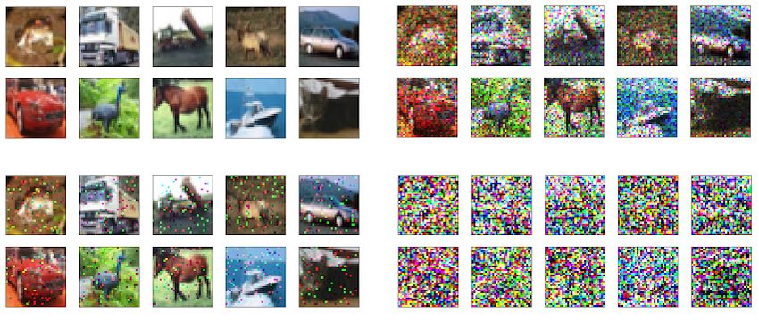
The following individuals certify that they have read, and recommend to the Fac-
ulty of Graduate and Postdoctoral Studies for acceptance, the thesis entitled:

Fault Injection in Machine Learning Applications

submitted by Niranjhana Narayanan in partial fulfillment of the requirements for
the degree of Master of Applied Science in Electrical and Computer Engineer-
ing.

Examining Committee:
Dr. Karthik Pattabiraman, Electrical and Computer Engineering, UBC
Supervisor
Dr. Sathish Gopalakrishnan, Electrical and Computer Engineering, UBC
Chair
Dr. Prashant Nair, Electrical and Computer Engineering, UBC
Supervisory Committee Member

                                       ii
Abstract

As Machine Learning (ML) has seen increasing adoption in safety-critical domains
(e.g., Autonomous Vehicles (AV)), the reliability of ML systems has also grown
in importance. While prior studies have proposed techniques to enable efficient
error-resilience (e.g., selective instruction duplication), a fundamental requirement
for realizing these techniques is a detailed understanding of the application’s re-
silience.
    The primary part of this thesis focuses on studying ML application resilience to
hardware and software faults. To this end, we present the TensorFI tool set, con-
sisting of TensorFI 1 and 2 which are high-level Fault Injection (FI) frameworks
for TensorFlow 1 and 2 respectively. With this tool set, we inject faults in Ten-
sorFlow programs and study important reliability aspects such as model resilience
to different kinds of faults, operator and layer level resilience of different models
or the effect of hyperparameter variations. We evaluate the resilience of 12 ML
applications, including those used in the autonomous vehicle domain. From our
experiments, we find that there are significant differences between different ML
applications and different configurations. Further, we find that applications are
more vulnerable to bit-flip faults than other kinds of faults. We conduct four case
studies to demonstrate some use cases of the tool set. We find the most and least
resilient image classes to faults in a traffic sign recognition model. We consider
layer-wise resilience and observe that faults in the initial layers of an application
result in higher vulnerability. In addition, we visualize the outputs from layer-
wise injection in an image segmentation model, and are able to identify the layer in
which faults occurred based on the faulty prediction masks. These case studies thus
provide valuable insights into how to improve the resilience of ML applications.

                                         iii
The secondary part of this thesis focuses on studying ML application resilience
to data faults (e.g. adversarial inputs, labeling errors, common corruptions/noisy
data). We present a data mutation tool, TensorFlow Data Mutator (TF-DM), which
targets different kinds of data faults commonly occurring in ML applications. We
conduct experiments using TF-DM and outline the resiliency analysis of different
models and datasets.

                                        iv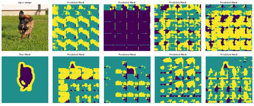
Lay Summary

Machine Learning (ML) is increasingly deployed in safety-critical systems. Fail-
ures or attacks on such systems (e.g. self driving cars) can have disastrous conse-
quences and so ensuring the reliability of its operations is important. Fault injection
FI is a popular method for assessing the reliability of applications.   In this thesis, we
first present a FI tool set consisting of TensorFI 1 and 2 for ML programs written in
TensorFlow. We then use the tool set to inject both software and hardware faults
in many ML applications and find valuable insights to improve the application’s
resilience. Finally, we present a data mutation tool, TensorFlow Data Mutator (TF-
DM) and use it to study the application’s resilience to data faults.

                                          v
Preface

This thesis is the result of work carried out by myself, in collaboration with my
supervisor, Prof. Karthik Pattabiraman, Zitao Chen, Dr. Bo Fang, Dr. Guanpeng
Li and Dr. Nathan DeBardeleben. All chapters are based on the work listed below.

    • Z. Chen, N. Narayanan, B. Fang, G. Li, K. Pattabiraman and N. DeBardeleben,
      “TensorFI: A Flexible Fault Injection Framework for TensorFlow Applica-
      tions”, 2020 IEEE 31st International Symposium on Software Reliability En-
      gineering (ISSRE).
      I was responsible for extending the original TensorFI 1 architecture designed
      and implemented by Zitao, Guanpeng, Karthik and Nathan, supporting more
      models and conducting experiments. Zitao and Karthik helped with feed-
      back, analysis and writing parts of the paper. Zitao and Bo helped with
      conducting experiments and provided technical support.

    • N. Narayanan and K. Pattabiraman, “TF-DM: Tool for Studying ML Model
      Resilience to Data Faults”, Proceedings of the 2nd International Workshop
      on Testing for Deep Learning and Deep Learning for Testing (DeepTest
      2021), colocated with ICSE 2021.

    • N. Narayanan, Z. Chen, B. Fang, G. Li, K. Pattabiraman and N. DeBardeleben,
      “Fault Injection for TensorFlow Applications”, in submission to a journal.
      I was responsible for conceiving the ideas, design and implementation of
      TF-DM and TensorFI 2 and conducting experiments, compiling the results
      and writing the paper (TensorFI 2 is included along with TensorFI 1 in this

                                        vi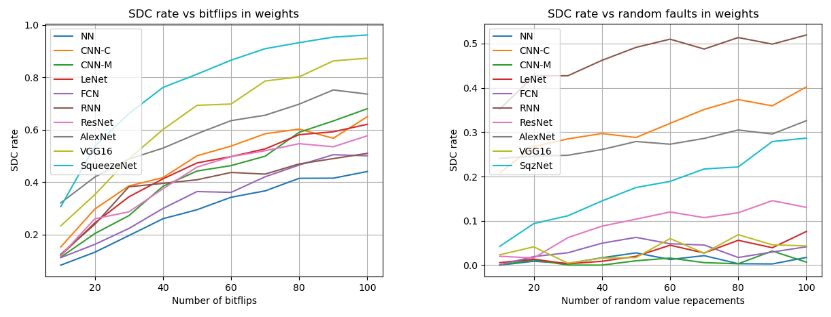
submission). Karthik was responsible for overseeing the project, providing
feedback and writing parts of the paper.

                                 vii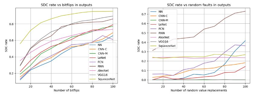
Table of Contents

Abstract . . . . . . . . . . . . . . . . . . . . . . . . . . . . . . . . . . . .    iii

Lay Summary . . . . . . . . . . . . . . . . . . . . . . . . . . . . . . . .          v

Preface . . . . . . . . . . . . . . . . . . . . . . . . . . . . . . . . . . . .     vi

Table of Contents . . . . . . . . . . . . . . . . . . . . . . . . . . . . . .      viii

List of Tables . . . . . . . . . . . . . . . . . . . . . . . . . . . . . . . . .   xii

List of Figures . . . . . . . . . . . . . . . . . . . . . . . . . . . . . . . .    xiii

List of Abbreviations . . . . . . . . . . . . . . . . . . . . . . . . . . . .      xvi

Acknowledgments . . . . . . . . . . . . . . . . . . . . . . . . . . . . . . xvii

1   Introduction . . . . . . . . . . . . . . . . . . . . . . . . . . . . . . .       1
    1.1   Motivation . . . . . . . . . . . . . . . . . . . . . . . . . . . . . .     1
    1.2   Approach . . . . . . . . . . . . . . . . . . . . . . . . . . . . . .       2
    1.3   Contributions . . . . . . . . . . . . . . . . . . . . . . . . . . . .      4

2   Background . . . . . . . . . . . . . . . . . . . . . . . . . . . . . . .         7
    2.1   ML Applications . . . . . . . . . . . . . . . . . . . . . . . . . .        7
    2.2   TensorFlow 1 and 2 . . . . . . . . . . . . . . . . . . . . . . . . .       8
    2.3   Fault Model . . . . . . . . . . . . . . . . . . . . . . . . . . . . .      9
          2.3.1   TensorFI tool set . . . . . . . . . . . . . . . . . . . . . .      9

                                         viii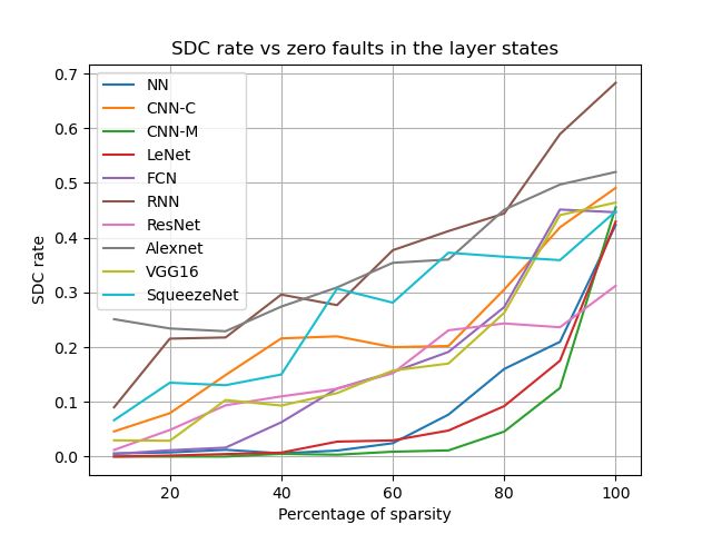
2.3.2   TF-DM tool . . . . . . . . . . . . . . . . . . . . . . . . .     10
          2.3.3   Evaluation Metric . . . . . . . . . . . . . . . . . . . . . .    11
    2.4   Related Work . . . . . . . . . . . . . . . . . . . . . . . . . . . .     11

3   Approach . . . . . . . . . . . . . . . . . . . . . . . . . . . . . . . . .     14
    3.1   Design Constraints . . . . . . . . . . . . . . . . . . . . . . . . .     14
    3.2   TensorFI 1 . . . . . . . . . . . . . . . . . . . . . . . . . . . . . .   15
          3.2.1   Design Alternatives . . . . . . . . . . . . . . . . . . . . .    15
          3.2.2   Implementation . . . . . . . . . . . . . . . . . . . . . . .     16
    3.3   TensorFI 2 . . . . . . . . . . . . . . . . . . . . . . . . . . . . . .   17
          3.3.1   Design Challenges . . . . . . . . . . . . . . . . . . . . .      17
          3.3.2   Design Alternatives . . . . . . . . . . . . . . . . . . . . .    18
          3.3.3   Implementation . . . . . . . . . . . . . . . . . . . . . . .     18
    3.4   Satisfying Design Constraints . . . . . . . . . . . . . . . . . . . .    20
    3.5   Configuration and Usage . . . . . . . . . . . . . . . . . . . . . .      21
    3.6   Summary . . . . . . . . . . . . . . . . . . . . . . . . . . . . . .      22

4   Evaluation of TensorFI . . . . . . . . . . . . . . . . . . . . . . . . .       23
    4.1   Experimental Setup . . . . . . . . . . . . . . . . . . . . . . . . .     23
          4.1.1   ML Applications . . . . . . . . . . . . . . . . . . . . . .      23
          4.1.2   ML Datasets . . . . . . . . . . . . . . . . . . . . . . . .      25
          4.1.3   Metrics . . . . . . . . . . . . . . . . . . . . . . . . . . .    25
          4.1.4   Experiments . . . . . . . . . . . . . . . . . . . . . . . .      26
    4.2   TensorFI 1 Results . . . . . . . . . . . . . . . . . . . . . . . . .     27
          4.2.1   RQ1: Error resilience for different injection modes . . . .      27
          4.2.2   RQ2: Error resilience under different error rates . . . . . .    29
          4.2.3   RQ3: SDC rates across different operators . . . . . . . . .      31
          4.2.4   GAN FI results . . . . . . . . . . . . . . . . . . . . . . .     32
    4.3   TensorFI 2 Results . . . . . . . . . . . . . . . . . . . . . . . . .     33
          4.3.1   RQ1: Error resilience for different injection modes and
                  fault types in the layer states (weights and biases) . . . . .   33
          4.3.2   RQ2: Error resilience for different injection modes and
                  fault types in the layer computations (outputs) . . . . . . .    36

                                          ix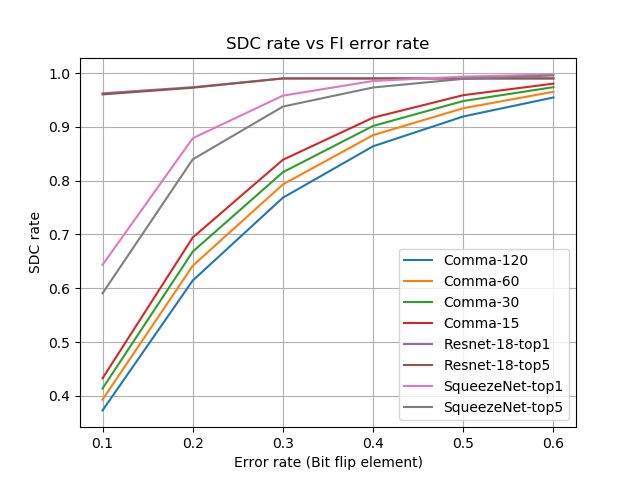
4.3.3   RQ3: Error resilience under zero faults in the layer states
                  (weight sparsity) . . . . . . . . . . . . . . . . . . . . . .     37
          4.3.4   RQ4: Error resilience under zero faults in the convolu-
                  tional layer states . . . . . . . . . . . . . . . . . . . . . .   39
    4.4   Overheads: TensorFI 1 vs 2 . . . . . . . . . . . . . . . . . . . . .      41
    4.5   Summary . . . . . . . . . . . . . . . . . . . . . . . . . . . . . .       43

5   Case Studies . . . . . . . . . . . . . . . . . . . . . . . . . . . . . . .      44
    5.1   TensorFI 1 . . . . . . . . . . . . . . . . . . . . . . . . . . . . . .    44
          5.1.1   Effect of Hyperparameter Variations . . . . . . . . . . . .       44
          5.1.2   Layer-Wise Resilience . . . . . . . . . . . . . . . . . . .       46
    5.2   TensorFI 2 . . . . . . . . . . . . . . . . . . . . . . . . . . . . . .    47
          5.2.1   Understanding resilience to bit-flips in a traffic sign recog-
                  nition model: Are certain classes more vulnerable? . . . .        47
          5.2.2   Visualizing resilience to bit-flips at lower levels of object
                  detection: Is it possible to identify the layer at which bit-
                  flips occur from analysing the faulty masks predicted? . .        49
    5.3   Summary . . . . . . . . . . . . . . . . . . . . . . . . . . . . . .       52

6   TensorFlow Data Mutator . . . . . . . . . . . . . . . . . . . . . . . .         53
    6.1   Implementation challenges . . . . . . . . . . . . . . . . . . . . .       53
          6.1.1   Handling different datasets . . . . . . . . . . . . . . . . .     53
          6.1.2   Using TensorFlow 2 . . . . . . . . . . . . . . . . . . . .        54
    6.2   Data mutators . . . . . . . . . . . . . . . . . . . . . . . . . . . .     54
          6.2.1   Data removal . . . . . . . . . . . . . . . . . . . . . . . .      55
          6.2.2   Data repetition . . . . . . . . . . . . . . . . . . . . . . .     55
          6.2.3   Data shuffle . . . . . . . . . . . . . . . . . . . . . . . . .    55
          6.2.4   Feature noise addition . . . . . . . . . . . . . . . . . . .      56
          6.2.5   Label error . . . . . . . . . . . . . . . . . . . . . . . . .     57
    6.3   Installation and Usage . . . . . . . . . . . . . . . . . . . . . . . .    57
    6.4   Evaluation . . . . . . . . . . . . . . . . . . . . . . . . . . . . . .    57
          6.4.1   Experimental configurations . . . . . . . . . . . . . . . .       58
          6.4.2   Results . . . . . . . . . . . . . . . . . . . . . . . . . . .     58

                                          x
6.5 Summary . . . . . . . . . . . . . . . . . . . . . . . . . . . . . . 63
7 Conclusion and Future Work . . . . . . . . . . . . . . . . . . . . . . 64
7.1 Summary . . . . . . . . . . . . . . . . . . . . . . . . . . . . . . 64
7.2 Lessons Learned . . . . . . . . . . . . . . . . . . . . . . . . . . 65
7.2.1 Graph duplication: An essential evil in TensorFI 1? . . . . 65
7.2.2 Injection failures at certain layers with TensorFI 2 . . . . . 66
7.2.3 Get a head start on the evaluation . . . . . . . . . . . . . 67
7.2.4 Extensive documentation always helps . . . . . . . . . . . 67
7.2.5 Improvements/additional features for all three tools . . . . 68
7.3 Future Work . . . . . . . . . . . . . . . . . . . . . . . . . . . . . 68
7.3.1 Evaluation on real-world ML systems . . . . . . . . . . . 68
7.3.2 Automated ways to improve the resilience upon detecting
vulnerabilities . . . . . . . . . . . . . . . . . . . . . . . . 69
7.3.3 Integrate injection capabilities for quantized models . . . 69
7.3.4 Comprehensive evaluation of the tool set . . . . . . . . . 70
7.3.5 A 3-dimensional metric for evaluation . . . . . . . . . . . 70
7.3.6 Improving the resiliency of the GTSRB dataset . . . . . . 71
Bibliography . . . . . . . . . . . . . . . . . . . . . . . . . . . . . . . . . 72
xiList of Tables
Table 2.1 Fault model for the TensorFI tool set . . . . . . . . . . . . . . 10
Table 3.1 List of fault types supported by TensorFI 1 . . . . . . . . . . . 21
Table 3.2 List of fault types supported by TensorFI 2 . . . . . . . . . . . 21
Table 3.3 List of analogous injection modes between TensorFI 1 and Ten-
sorFI 2 . . . . . . . . . . . . . . . . . . . . . . . . . . . . . . 22
Table 4.1 ML applications and datasets used for TensorFI 1 evaluation.
The baseline model accuracies are also provided. . . . . . . . . 24
Table 4.2 ML applications and datasets used for TensorFI 2. . . . . . . . 24
Table 4.3 SDC rates for bitflips in the NN-MNIST model . . . . . . . . . 40
Table 4.4 Overheads for the program without FI in TensorFlow 1 and Ten-
sorFlow 2 (baseline); and with FI in TensorFI 1 and TensorFI
2 . . . . . . . . . . . . . . . . . . . . . . . . . . . . . . . . . 41
Table 5.1 Layerwise resilience in a CNN model . . . . . . . . . . . . . . 46
Table 6.1 ML applications and datasets used for evaluation. . . . . . . . 58
Table 6.2 Accuracies before and after shuffling the dataset. . . . . . . . . 60
xiiList of Figures
Figure 3.1 Working methodology of TensorFI 1: The green nodes are the
original nodes constructed by the TensorFlow graph, while the
nodes in red are added by TensorFI 1 for FI purposes. . . . . . 16
Figure 3.2 Working methodology of TensorFI 2: The conv 1 layer is cho-
sen for both weight FI (left) and activation state injection (right).
The arrows in red show the propagation of the fault. . . . . . . 20
Figure 4.1 Example of SDCs observed in different ML applications. Left
box - steering model. Right box - image misclassifications. . . 27
Figure 4.2 SDC rates under single bit-flip faults (from oneFaultPerRun
and dynamicInstance injection modes). Error bars range from
±0.19% to ±2.45% at the 95% confidence interval. . . . . . . 28
Figure 4.3 SDC rates for various error rates (under bit flip element FI). Er-
ror bars range from ±0.33% to ±1.68% at the 95% confidence
interval. . . . . . . . . . . . . . . . . . . . . . . . . . . . . . 29
Figure 4.4 SDC rates for various error rates (under random value replace-
ment FI). Error bars range from ±0.13% to ±1.59% at the 95%
confidence interval. . . . . . . . . . . . . . . . . . . . . . . . 30
Figure 4.5 SDC rates of different operators under bit-flip FI in the CNN
model). Error bars range from ±0.3077% to ±0.9592% at
95% confidence interval. . . . . . . . . . . . . . . . . . . . . 31
xiiiFigure 4.6 Generated images of the digit 8 in the MNIST dataset under
different configurations for GANs. Top row represents the
Rand-element model, while bottom row represents the single
bit-flip model. Left center is with no faults. . . . . . . . . . . 32
Figure 4.7 SDC rates under bit-flip faults in weights and biases (from
single injection modes). Error bars range from ±0.53% to
±3.02% at the 95% confidence interval. . . . . . . . . . . . . 34
Figure 4.8 SDC rates for bit-flips and random value replacement faults in
the layer states. Error bars range from ±0.97% to ±3.09%
for bit-flips and ±0.01% to ±0.98% for random value replace-
ment faults at the 95% confidence interval. . . . . . . . . . . 35
Figure 4.9 SDC rates under single bit-flip faults in activations. Error bars
range from ±0.22% to ±0.85% at the 95% confidence interval. 36
Figure 4.10 SDC rates for bit-flips and random value replacement faults in
the layer outputs. Error bars range from ±0.06% to ±3.08%
for bit-flips and ±0.01% to ±2.31% for random value replace-
ment faults at the 95% confidence interval. . . . . . . . . . . 37
Figure 4.11 SDC rates under zero faults in weights and biases. Error bars
range from ±0.05% to ±3.06% at the 95% confidence interval. 38
Figure 4.12 SDC rates under zero faults in the convolutional layer states.
Error bars range from ±0.01% to ±2.75% at the 95% confi-
dence interval. . . . . . . . . . . . . . . . . . . . . . . . . . 39
Figure 5.1 SDC rates in different variations of the NN model. Error bars
range from ±0.7928% to ±0.9716% at the 95% confidence
interval. . . . . . . . . . . . . . . . . . . . . . . . . . . . . . 45
Figure 5.2 Accuracy in different variations of the NN model. . . . . . . . 45
Figure 5.3 The number of correct predictions for each class in GTSRB for
different numbers (legend) of bit-flips in the first convolutional
layer. . . . . . . . . . . . . . . . . . . . . . . . . . . . . . . 48
Figure 5.4 Top 5 most (upper) and least resilient (lower) traffic signs and
their GTSRB classes to bit-flips in the first convolutional layer. 49
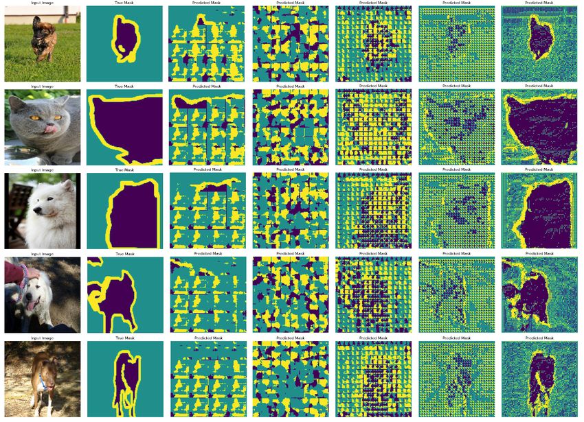
xivFigure 5.5 Predicted faulty masks for bit-flips in different layers of the
image segmentation model. The first column is the original
image, the second column is the predicted mask in the absence
of faults. The remaining columns show the predicted mask
after a fault in the ith convolutional layer, where i ranges from
1 to 5. . . . . . . . . . . . . . . . . . . . . . . . . . . . . . . 51
Figure 5.6 8 instances of faulty masks predicted for the same fault config-
uration in the first layer for the same test image (far left). . . . 52
Figure 6.1 Different types of noise injected into the CIFAR-10 dataset. . 56
Figure 6.2 SDC rates in different ML applications for data removal. Error
bars range from ±0.45% to ±3.09% at the 95% confidence
interval. . . . . . . . . . . . . . . . . . . . . . . . . . . . . . 59
Figure 6.3 SDC rates in different ML applications for data repetition. Er-
ror bars range from ±0.47% to ±3.09% at the 95% confidence
interval. . . . . . . . . . . . . . . . . . . . . . . . . . . . . . 59
Figure 6.4 SDC rates in different ML applications for noise addition. Er-
ror bars range from ±0.14% to ±2.89% at the 95% confidence
interval. . . . . . . . . . . . . . . . . . . . . . . . . . . . . . 61
Figure 6.5 SDC rates in different ML applications for data mislabel. Error
bars range from ±0.58% to ±3.06% at the 95% confidence
interval. . . . . . . . . . . . . . . . . . . . . . . . . . . . . . 62
Figure 6.6 Single side targeted misclassifications. Error bars range from
±0.52% to ±3.01% at the 95% confidence interval. . . . . . . 62
Figure 6.7 Double side targeted misclassifications. Error bars range from
±0.55% to ±2.68% at the 95% confidence interval. . . . . . . 63
xvList of Abbreviations
API Application Programming Interface
AV Autonomous Vehicles
DNN Deep Neural Network
FI Fault Injection
FIT Failures-In-Time
GUI Graphical User Interface
IOT Internet of Things
ML Machine Learning
OS Operating System
SDC Silent Data Corruption
SLOC Source Lines of Code
xviAcknowledgments
First and foremost, I would like to thank my advisor Dr. Karthik Pattabiraman
for his constant guidance and support throughout my Masters. He has helped me
try out new ideas and consistently provided direction to build on top of them and
execute to fruition. During the difficult times when progress seemed elusive, his
knowledge and enthusiasm provided me with motivation; and his patience and fault
tolerance (pun intended) provided me with courage to keep persisting on my path.
Along with my advisor, I would like to thank my thesis examining committee,
Dr. Sathish Gopalakrishnan and Dr. Prashant Nair, for their thought-provoking
questions and valuable feedback on this thesis. I would also like to thank my
colleagues at the Dependable Systems Lab for all the constructive feedback and
insightful discussions.
I would like to thank my friends here at Vancouver and in different parts of the
world who have helped me with preparing for and getting through graduate school.
Special thanks to choof who has been with me through the highs and lows, helping
me cope with the stress that came with graduate studies.
Last but not least, I would like to thank my parents without whom this would
never have been possible. They have provided me with unconditional love and sup-
port throughout my life, encouraging me to pursue my goals despite any obstacles.
xviiChapter 1
Introduction
1.1 Motivation
In the past decade, advances in Machine Learning (ML) have increased its deploy-
ment across safety-critical domains such as Autonomous Vehicles (AVs) [28] and
aircraft control [50]. In these domains, it is critical to ensure the reliability of the
ML algorithm and its implementation, as faults can lead to loss of life and prop-
erty. Moreover, there are often safety standards in these domains that prescribe the
maximum allowed failure rate. For example, in the AV domain, the ISO 26262
standard mandates that the FIT rate (Failures in Time) of the system be no more
than 10, i.e., at most 10 failures in a billion hours of operation [22], in order to
achieve ASIL-D levels of certification. Therefore, there is a compelling need to
build efficient tools to (1) test and improve the reliability of ML systems, and (2)
evaluate their failure rates in the presence of different fault types. Faults or attacks
anywhere in the ML pipeline (at the hardware, software or data level) can hence
have disastrous consequences [30, 33, 35, 44, 56, 64, 71].
It has thus become a necessity to assess the dependability of the ML models,
before they are deployed in safety-critical applications. The traditional way to ex-
perimentally assess the reliability of a system is Fault Injection (FI). FI can be im-
plemented at the hardware level or software level. Software-Implemented FI (also
known as SWiFI) has lower costs, is more controllable, and easier for developers
to deploy [46]. Therefore, SWiFI has become the dominant method to assess a sys-
1tem’s resilience to both hardware and software faults. There has been a plethora of
SWiFI tools such as NFTape [73], Xception [32], GOOFI [25], LFI [61], LLFI [75],
PINFI [78]. These tools operate at different levels of the system stack, from the
assembly code level to the application’s source code level. In general, the higher
the level of abstraction of the FI tool, the easier it is for developers to work with,
and use the results from the FI experiments [46].
Due to the increase in popularity of ML applications, there have been many
frameworks developed for writing them. An example is TensorFlow [24], which
was released by Google in 2017. Other examples are PyTorch [66] and CNTK [3].
These frameworks allow the developer to “compose” their application as a se-
quence of operations, which are connected either sequentially or in the form of
a graph. The connections represent the data-flow and control dependencies among
the operations. While the underlying implementation of these frameworks is in
C++ or assembly code for performance reasons, the developer writes their code
using high-level languages (e.g., Python). Thus, there is a need for a specialized FI
framework that can directly inject faults into the ML application. We address this
need through our TensorFI tool set introduced in this thesis.
While TensorFI can be used to study the effects of hardware and software faults
on ML applications, faults can also arise in the input data. However, there is no
comprehensive tool that produces an end-to-end evaluation of an ML application
for faults in input data. At the data level, the faults can be categorized into (1)
intentional arising due to adversarial attacks, and (2) unintentional, arising due to
concept drift or noisy data. To mitigate the effects of adversarial attacks, users may
need to train their models in the presence of varying amounts of adversarial data.
Further, users may want to understand how resilient their models are to the effects
of concept drift and data corruption. We address this need through our TensorFlow
Data Mutator (TF-DM) tool.
1.2 Approach
In this thesis, we present 3 tools, TensorFI 1, TensorFI 2 and TF-DM for Tensor-
Flow applications. Using these tools, we provide an analytical understanding on
the error resilience of different ML applications under different kinds of faults at
2the hardware, software and data levels.
We first present the TensorFI tool set that consists of TensorFI 1 [15] and Ten-
sorFI 2 [16]. They can inject both hardware and software faults in either the outputs
of TensorFlow operators (TensorFI 1) or the states and activations of model layers
(TensorFI 2). The main advantage of these injectors over traditional SWiFI frame-
works is that they directly operate on either the TensorFlow operators and graph or
the layers and model, and hence their results are readily accessible to developers.
We focus on TensorFlow as it is the most popular framework used today for ML
applications [23], though our techniques are not restricted to TensorFlow.
The differences between TensorFI 1 and 2 are as follows. First, TensorFI 1
operates only on TensorFlow 1 applications that had an explicit graph representa-
tion. However, TensorFlow 2 applications do not necessarily have an underlying
data-flow graph. Second, TensorFI 1 can only inject into the results of individ-
ual operators in the TensorFlow graph. In contrast, TensorFI 2 can also be used
to inject faults into the model parameters such as weights and biases as well as
the outputs of different activation or hidden layer states. Both TensorFI 1 and 2
perform interface-level FI [53, 54]. We explain the detailed operation of the two
injectors below.
TensorFI 1 works by first duplicating the TensorFlow graph and creating a FI
graph that parallels the original one. The operators in the FI graph mirror the func-
tionality of the original TensorFlow operators, except that they have the capability
to inject faults based on the configuration parameters specified. These operators
are implemented by us in Python, thereby ensuring their portability. Moreover, the
FI graph is only invoked during fault injection, and hence the performance of the
original TensorFlow graph is not affected (when faults are not injected). Finally,
because we do not modify the TensorFlow graph other than to add the FI graph,
external libraries can continue to work.
However, TensorFI 1 does not work for TensorFlow 2 applications because
TensorFlow 2 is based on the eager execution model, and graphs are not con-
structed by default. TensorFI 2 addresses this challenge by using the Keras APIs to
intercept the tensor states of different layers directly for fault injection. Graph du-
plication is avoided along with the overheads it incurs (we quantitatively evaluate
the overheads later in Section 4). TensorFI 2 is also designed for portability and
3compatibility with external libraries.
While prior work has studied the error resilience of ML models by building
customized fault injection tools [36, 57, 70, 72], these tools are usually tailored
for a specific set of programs and are not applicable to general ML programs. In
contrast, the TensorFI tool set contains generic and configurable fault injection
tools that are able to inject faults in a wide range of ML programs written using
TensorFlow 1 and 2.
Finally, we present our tool TensorFlow Data Mutator (TF-DM) [13], which
supports three types of data mutators, so users can perform a holistic assessment
of their ML models to the effects of different data faults. TensorFI allows users
to (1) remove parts of the training or test data to understand the minimal amount
of data that is required for their model, (2) mislabel parts of the data to see the
consequences of both targeted and untargeted misclassifications from adversarial
attacks, and (3) add different kinds of noise to the data to emulate the effects of
noisy inputs. Currently, TensorFI has the capability to mutate different datasets
from the Keras and TensorFlow libraries, including support for large scale datasets
such as ImageNet.
1.3 Contributions
To summarize, we first list the contributions made with our TensorFI tool set and
then our TF-DM tool.
Chapters 3, 4 and 5 of this thesis focus on the TensorFI tool set where we:
• Propose generic FI techniques to inject faults in the TensorFlow 1 and 2
frameworks.
• Implement the FI techniques in TensorFI 1 and 2, which allow (1) easy con-
figuration of FI parameters, (2) portability, and (3) minimal interference with
the program.
• Evaluate the tools on 12 ML applications, including Deep Neural Network
(DNN) applications used in AVs, across a range of FI configurations (e.g.,
fault types, error rates). From our experiments, we find that there are signif-
icant differences due to both individual ML applications, as well as different
4configurations. Further, applications are more vulnerable to bit-flip faults
than other kinds of faults in both the tools. Finally, TensorFI 2 was more
than twice as fast as TensorFI 1 for injecting similar faults.
• Conduct four case studies, two for each tool, to demonstrate some of the use
cases of the tool. We find the most and least resilient image classes in the
GTSRB dataset [45] from fault injection in a traffic sign recognition model.
We consider layer-wise resilience in two of our case studies, and observe
that faults in the initial layers of an application result in higher vulnerability.
In addition, we visualize the outputs from layer-wise injection in an image
segmentation model, and are able to identify the layer in which faults oc-
curred based on the faulty prediction masks. These case studies thus provide
valuable insights into how to improve the resilience of ML applications.
Chapter 6 focuses on TF-DM where we:
• Present the background of the different faults and attacks at the data level in
ML applications,
• Discuss the challenges in modeling the various fault models to corresponding
data mutators in a framework,
• Implement five mutators in an automated tool TF-DM,
• Perform detailed evaluation of TF-DM on 7 ML models and 3 datasets com-
monly used in the literature. From our experiments, we find that different
models have varying resilience to the same type of data fault. In general,
resilience to data faults decreases with increasing model and dataset com-
plexity. We also find that certain classes of the CIFAR-10 dataset are more
vulnerable to targeted misclassifications.
Our findings thus provide an analytical understanding of the error resilience in
different ML applications due to faults at the hardware, software and data level.
Further, we are able to corroborate previous work such as finding that there is
a decreasing propagation probability across layers, as faults that occur in earlier
layers have a higher probability of propagating to other layers and spreading [57]
5vs. Sections 5.1.2 and 5.2.2. We find some new results comparing resilience across
different models, datasets, fault types, fault configurations and injection modes. In
addition, we also provide usable tools to identify the vulnerable artifacts in an ML
application and demonstrate the utility of the tools with case studies. Our tools are
open source and available at [13, 15, 16]. These contributions thus help in building
error-resilient applications in the ML domain.
6Chapter 2
Background
In this chapter, we start by explaining the general structure of ML applications.
We follow up with the differences in TensorFlow 1 and 2 applications necessary to
appreciate the developed tools. We then explain the fault model we assume for the
TensorFI tool set and the TF-DM tool. We conclude with related work in the area
of ML reliability.
2.1 ML Applications
An ML model takes an input that contains specific features to make a prediction.
Prediction tasks can be divided into classification and regression. The former is
used to classify the input into categorical outputs (e.g., image classification). The
latter is used to predict dependent variable values based on the input. ML models
can be either supervised or unsupervised. In the supervised setting, the training
samples are assigned with known labels (e.g., linear regression, neural network),
while in an unsupervised setting there are no known labels for the training data
(e.g., k-means, kernel density estimation).
An ML model typically goes through two phases: 1) training phase where the
model is trained to learn a particular task; 2) inference phase where the model is
used for making predictions on test data. The parameters of the ML model are
learned from the training data, and the trained model is evaluated on the test data,
which represents the unseen data.
72.2 TensorFlow 1 and 2
TensorFlow abstracts the operations in an ML application thus allowing program-
mers to focus on the high-level programming logic. In TensorFlow 1, programmers
use the built-in operators to construct the data-flow graph of the ML algorithm dur-
ing the training phase. Once the graph is built, it is not allowed to be modified.
During the inference phase, data is fed into the graph through the use of place-
holder operators, and the outputs of the graph correspond to the outputs of the ML
algorithm. TensorFlow 1 version was difficult to learn and use for ML practition-
ers, with users having to deal with graphs, sessions and follow a meticulous method
of building models [12].
With TensorFlow 2, eager execution was introduced making it more Pythonic.
Graphs are not built by default but can be created with tf.function as they are good
for speed. TensorFlow 2 embraces the Keras APIs for building models making it
easier and more flexible for users. In TensorFlow 2, programmers define the ML
model layer by layer and these layer objects have training and inference features.
When data is fed into the ML algorithm, the operations in the layers are immedi-
ately executed.
Both versions of TensorFlow also provide a convenient Python language inter-
face for programmers to construct and manipulate the data-flow graphs. Though
other languages are also supported, the dominant use of TensorFlow is through its
Python interface. Note however that the majority of the ML operators and algo-
rithms are implemented as C/C++ code, and have optimized versions for different
platforms. The Python interface simply provides a wrapper around these C/C++
implementations.
For example, the following code samples show how tensors are treated in Ten-
sorFlow 1 vs. TensorFlow 2.
# TensorFlow 1 # TensorFlow 2
# SYMBOLIC # CONCRETE
a = tf.constant(2) a = tf.constant(3)
b = tf.constant(5) b = tf.constant(7)
c = a * b c = a * b
with tf.Session() as sess: print(c) # eagerly executed
print(sess.run(c))
8We can see that we do not need to use sessions any more in TensorFlow 2 as
we can work with tensors imperatively just as we would with say NumPy arrays,
as a result of adopting the eager execution model.
2.3 Fault Model
2.3.1 TensorFI tool set
In the TensorFI tool set, we consider both hardware faults and software faults that
occur in TensorFlow programs.
TensorFI 1 operates at the level of TensorFlow graph operations. We abstract
the faults to the operators’ interfaces. Thus, we assume that a hardware or software
fault that arises within the TensorFlow operators, ends up corrupting (only) the
respective outputs. However, we do not make assumptions on the nature of the
output’s corruption. For example, we consider that the output corruption could be
manifested as either a random value replacement [59] or as a single bit-flip [36, 57,
70, 72].
TensorFI 2 operates at the TensorFlow model level. We abstract faults either to
the interfaces of the model layers or to the model parameters. TensorFI 2 can inject
faults into the layer states i.e. the weights and biases. TensorFI 2 models two kinds
of faults. (1) Transient hardware faults during computation, which can alter the
activations or outputs of each layer. (2) Faults that can occur due to rowhammer at-
tacks [44], i.e., an attacker performing specific memory access patterns can induce
persistent and repeatable bit corruptions from software. The vulnerable parameters
tend to be larger objects (greater than 1MB) in memory, and these are usually page
aligned allocations such as weights, biases.
Table 2.1 shows the faults considered by both TensorFI 1 and 2, and how they
are modeled. We make three assumptions about faults. First, we assume that the
faults do not modify the structure of the TensorFlow graph or model (since Ten-
sorFlow assumes a static computational graph) and that the inputs provided into
the program are correct, because such faults are extraneous to TensorFlow. Other
work has considered errors in inputs[26, 68]. Second, we assume that the faults
do not occur in the ML algorithms or the implementation itself. This allows us to
9Table 2.1: Fault model for the TensorFI tool set
TensorFI 1 TensorFI 2
Software faults,
Software faults
transient hardware
Source of fault and transient
faults, rowhammer
hardware faults
attacks
Layer outputs
Modeling of fault Operator outputs and layer state
(weights)
Bitflips, zeros and Bitflips, zeros and
Fault types random value re- random value re-
placement placement
compare the output of the FI runs with the golden runs, to determine if the fault
has propagated and a Silent Data Corruption (SDC) has occurred. An important
assumption we make is that we focus only on the cases where the inference was
correct in the fault free situation, but incorrect after the fault. It could be possi-
ble that the reverse also happens i.e., an incorrectly classified input produces the
correct result after faults. However, we eliminate this consideration by our defini-
tion of our SDC metric, and is hence out of scope for our thesis. Finally, we only
consider faults during the inference phase of the ML program. This is because
training is usually a one-time process and the results of the trained model can be
checked. Inference, however, is executed repeatedly with different inputs, and is
hence much more likely to experience faults. This fault model is in line with other
related work [36, 57, 70, 72].
2.3.2 TF-DM tool
In the TF-DM tool, we consider data faults that occur in the input data fed to
an ML application. We use the term data layer to refer to these different inputs.
Examples include datasets such as MNIST, CIFAR10, ImageNet. Our goal is to
build a framework to study model resilience in the presence of both unintentional
and intentional faults in the data layer. We present examples of the two fault types
we consider below.
10Intentional Data Faults
Adversarial attacks: It has been shown that inputs with certain modifications that
are imperceptible to the human eye when passed through the ML algorithm get
grossly misclassified [30, 31, 63, 64, 71, 74]. Crafting such inputs to fool the
system is called an adversarial attack.
Unintentional Data Faults
Common corruptions and noisy data: There may be certain inputs that cause mis-
classification in a neural network. Common corruptions such as blur, tilts, fog,
noise or even changes in brightness have been shown to lower accuracy of the
DNNs [42]. There could also be natural adversarial examples where the DNN
classifies genuine unperturbed images incorrectly because of the shape and envi-
ronment of the object [43].
We note that two of the three assumptions we made for TensorFI hold for the
data faults as well. These are that the faults (i) do not modify the structure of
the TensorFlow graph or model and (ii) do not occur in the ML algorithms or the
implementation itself. However, we now consider the data faults occurring during
the training phase and in the inputs fed into the ML program. This is because the
fault types we have considered (adversarial inputs, noisy data) occur in the data
collected for training and our goal is to study the model resilience after retraining
with faulty data. This fault model is in line with other work in the area [49, 59].
2.3.3 Evaluation Metric
We use Silent Data Corruption (SDC) rate as the metric for evaluating the resilience
of ML applications in both the TensorFI tool set and the TF-DM tool. An SDC is
a wrong output that deviates from the expected output of the program. SDC rate is
the fraction of the injected faults that result in SDCs.
2.4 Related Work
Several studies have attempted to evaluate the error resilience of ML applications
through FI [27, 29]. However, such FI techniques are limited to the specific ap-
11plication being studied, unlike TensorFI that is able to perform FI on generic ML
applications.
In the hardware faults space, there has been significant work to investigate
the resilience of deep neural networks (DNN) to transient hardware faults (soft
errors) by building fault injectors [36, 57, 70, 72]. Li et al. build a fault injector by
using the tiny-CNN framework [57]. Reagen et al. design a generic framework for
quantifying the error resilience of ML applications [70]. Sabbagh et. al develop
a framework to study the fault resilience of compressed DNNs [72]. Chen et al.
introduce a technique to efficiently prune the hardware FI space by analyzing the
underlying property of ML models [36]. PyTorchFI [60] is a FI tool for DNNs,
used to mutate the weights or neurons in PyTorch applications, which is another
ML framework.
In the software faults space, research applying conventional software tech-
niques have seen various forms of success in evaluating different aspects of the
ML model. Mutation testing [47, 59], differential fuzzing [69], metamorphic test-
ing [39, 62, 82], whitebox [67] and blackbox testing tools [79] for ML have been
developed.
In the data faults space, there has been research in increasing the neuronal
coverage of the ML model by subjecting it to a diverse data set with the goal of
improved model prediction. DeepTest [76] generates new test data under different
transformations, and retrains the DNN with them to increase and diversify neu-
ron coverage and make the model robust. DeepMutation [59] is a mutation test-
ing framework for deep learning systems that evaluates the efficacy of test data in
DNNs to find weaknesses in the model by mutation testing. This involves chang-
ing the model or data to determine if the test data are still able to perform in the
presence of mutations, and if not, locate the source of errors. In recent work, Ja-
hangirova et al. [49] conduct an empirical evaluation of all the DeepMutation op-
erators taking into account the stochastic nature of the training process and identify
a subset of effective mutation operators with the associated configurations.
In contrast to the individual FI tools in the hardware, software and data faults
space, our three tools target a broader range of ML applications and are indepen-
dent of the underlying hardware platforms used. To the best of our knowledge,
there are no frameworks for quantitatively assessing the model resilience to faults
12at all the three levels. We aim to fill this gap with our TensorFI tool set which en-
ables the injection of hardware and software faults and TF-DM which enables the
injection of data faults, thus providing the capability to evaluate model resilience in
the presence of faults at all three levels. Finally, to the best of our knowledge, there
are no fault injection or data mutation tools for applications written in TensorFlow.
We also address this need with our three tools.
13Chapter 3
Approach
We start this chapter by articulating the common design constraints for the Ten-
sorFI tool set. We then discuss the design alternatives considered, and then present
the design of TensorFI 1 and 2 to satisfy the design constraints.
3.1 Design Constraints
We adhere to the following three constraints in the design of the TensorFI tool set.
• Ease of Use and Compatibility: The injectors should be easy-to-use and require
minimal modifications to the application code. We also need to ensure compat-
ibility with third-party libraries that may either construct the TensorFlow graph,
or use the model directly.
• Portability: Because TensorFlow may be pre-installed on the system, and each
individual system may have its own TensorFlow version, we should not assume
the programmer is able to make any modifications to TensorFlow. While pro-
viding Docker images for the tool can partially alleviate this issue, we need to
consider the case where the users may want to use a specific version of Tensor-
Flow because of other dependencies. We also want to provide a tool that does
not make any assumptions about the underlying system architecture on which the
OS runs, and so we consider portability to still be an important design constraint.
14• Minimal Interference: First, the injection process should not interfere with the
normal execution of the TensorFlow graph or model when no faults are injected.
Further, it should not make the underlying graph or model incapable of being
executed on GPUs or parallelized due to the modifications it makes. Finally, the
FI process should be reasonably fast.
3.2 TensorFI 1
3.2.1 Design Alternatives
Based on the design constraints in the previous section, we identified three poten-
tial ways to inject faults in the TensorFlow 1 graph. The first and perhaps most
straightforward method was to modify TensorFlow operators in place with FI ver-
sions. The FI versions would check for the presence of runtime flags and then
either inject the fault or continue with the regular operation of the operator. This is
similar to the method used by compiler-based FI tools such as LLFI [58]. Unfortu-
nately, this method does not work with TensorFlow graphs because the underlying
operators are implemented and run as C/C++ code, and cannot be modified.
A second design alternative is to directly modify the C++ implementation of
the TensorFlow graph to perform FIs. While this would work for injecting faults,
it violates the portability constraint as it would depend on the specific version of
TensorFlow being used and the platform it is being executed on. Further, it would
also violate the minimal inference constraint as the TensorFlow operators are opti-
mized for specific platforms (e.g., GPUs), and modifying them would potentially
break the platform-specific optimizations and may even slow down the process.
The third alternative is to directly inject faults into the higher-level APIs ex-
posed by TensorFlow rather than into the dataflow graph. The advantage of this
method would be that one can intercept the API calls and inject different kinds of
faults. However, this method would be limited to user code that uses the high-level
APIs, and would not be compatible with libraries that manipulate the TensorFlow
graph, violating the ease of use and compatibility constraint.
153.2.2 Implementation
To satisfy the design constraints outlined earlier, TensorFI 1 operates directly on
TensorFlow graphs. The main idea is to create a replica of the original TensorFlow
graph but with new operators. The new operators are capable of injecting faults
during the execution of the operators and can be controlled by an external config-
uration file. Further, when no faults are being injected, the operators emulate the
behavior of the original TensorFlow operators they replace.
Because TensorFlow does not allow the dataflow graph to be modified once it is
constructed, we need to create a copy of the entire graph, and not just the operators
we aim to inject faults into. The new graph mirrors the original one, and takes the
same inputs as it. However, it does not directly modify any of the nodes or edges of
the original graph and hence does not affect its operator. At runtime, a decision is
made as to whether to invoke the original TensorFlow graph or the duplicated one
for each invocation of the ML algorithm. Once the graph is chosen, it is executed
to completion at runtime.
TensorFI 1 works in two phases. The first phase instruments the graph, and
creates a duplicate of each node for FI purposes. The second phase executes the
graph to inject faults at runtime, and returns the corresponding output. Note that
the first phase is performed only once for the entire graph, while the second phase
is performed each time the graph is executed (and faults are injected). Figure 3.1
shows an example of how TensorFI 1 modifies a TensorFlow graph. Because our
goal is to illustrate the workflow of TensorFI 1, we consider a simple computation
rather than a real ML algorithm.
Figure 3.1: Working methodology of TensorFI 1: The green nodes are the
original nodes constructed by the TensorFlow graph, while the nodes in
red are added by TensorFI 1 for FI purposes.
16In the original TensorFlow graph, there are two operators, an ADD operator
which adds two constant nodes “Const 1” and “Const 2”, and a MUL operator,
which multiplies the resulting value with that from a placeholder node. A place-
holder node is used to feed data from an external source such as a file into a Ten-
sorFlow graph, and as such represents an input to the system. A constant node
represents a constant value. TensorFI 1 duplicates both the ADD and MUL oper-
ators in parallel to the main TensorFlow graph, and feeds them with the values of
the constant nodes as well as the placeholder node. Note that however there is no
flow of values back from the duplicated graph to the original graph, and hence the
FI nodes do not interfere with the original computation performed by the graph.
The outputs orig. and faulty represent the original and fault-injected values respec-
tively.
Prior to the FI process, TensorFI 1 instruments the original TensorFlow graph
to create a duplicate graph, which will then be invoked during the injection process.
At runtime, a dynamic decision is made as to whether we want to compute the orig.
output or the faulty output. If the orig. output is demanded, then the graph nodes
corresponding to the original TensorFlow graph are executed. Otherwise, the nodes
inserted by TensorFI 1 are executed and these emulate the behavior of the original
nodes, except that they inject faults. For example, assume that we want to inject
a fault into the ADD operator. Every other node inserted by TensorFI 1 would
behave exactly like the original nodes in the TensorFlow graph, with the exception
of the ADD operator which would inject faults as per the configuration.
3.3 TensorFI 2
3.3.1 Design Challenges
In TensorFlow 1, the session objects contain all the information regarding the graph
operations and model parameters. In TensorFlow 2, there is no graph built by
default as the eager execution model is adopted. This means that nodes in the
graph can no longer be used as the injection target by the fault injector. Instead,
the TensorFlow 2 models expose the corresponding layers that store the state and
computation of the tensor variables in it. Since these layers are representative of
17the different operations in TensorFlow, they are chosen as the injection target in
TensorFI 2.
In addition, TensorFlow 2 models can be built in three different ways - using
the sequential, functional and the sub-classing Keras APIs. The design of the FI
framework should be such that faults can be injected into the model regardless of
the method used to define it.
3.3.2 Design Alternatives
We considered two alternate approaches in the design of TensorFI 2. The first is
to create custom FI layers that duplicate the original layers to inject the incoming
tensors with the specified faults accordingly and pass it on to the next layer in
the model. This mimics the TensorFI 1 approach of creating a copy of the FI
operations in the graph. However, this approach incurs high overheads. While this
was the only feasible approach for TensorFI 1 because of the static computation
graph model adopted by TensorFlow 1, it is not so for TensorFlow 2. So we do not
adopt this approach.
The second design alternative uses eager execution to inject faults. Once the
model starts execution, each layer is checked whether it is chosen for FI. If a par-
ticular layer is chosen, the execution passes control to the injection function, which
injects the specified faults into the layer outputs. Unfortunately, this approach only
works for the sequential models, and not for models using non-linear topologies
such as the ResNet model. So we do not adopt this approach.
3.3.3 Implementation
ML models are made up of input data, weight matrices that are learned during train-
ing, and activation matrices that are computed from the weights and data. TensorFI
2 is capable of injecting faults into two different targets in any layer. The first is
the layer state or weight matrices that holds the learned model parameters such as
the weights and biases. This is to allow emulation of hardware and software faults
in these parameters.
In TensorFI 2, we use the Keras Model API [17] to retrieve the trained weights
and biases of the specified layer of the model given by the user, and use Tensor-
18Flow 2 operators (such as stack, flatten, assign) to retrieve and inject the parameters
according to the specified faults and store it back to observe the faulty inference
runs. By this method, the implementation is general enough to work with pro-
grams that use any of the three methods for building models in TensorFlow 2. The
supported mutations include injecting bit-flips in these tensor values, replacing the
tensor values with zeros or random values.
The second injection target is the layer computation or activation matrices,
which hold the output states of the layers. This is to allow emulation of hardware
transient faults that can arise in the computation units. In TensorFI 2, we use the
Keras backend API to directly intercept the tensor states of the layers chosen for
FI. For each layer where faults are to be injected, two Keras functions are modeled
before and after the injection call. The first contains the executed model outputs up
to that particular layer for the given test input and is taken as the injection target to
be operated on. These are the retrieved activation states, and faults are injected into
these tensor values and passed into the second function that models the subsequent
layers. For bit-flip faults, the bit position to be flipped can either be chosen prior to
injection or determined at runtime.
Modifying the layer states is static and is done before the inference runs. This
is illustrated in the left of Figure 3.2. The layers “conv 1”, “maxpool 1” and
“dense 1” are part of a larger convolutional network. Let us suppose the first con-
volution layer “conv 1” states are chosen for injection. TensorFI 2 then injects the
weights or biases of this layer and stores back the faulty parameters in the model.
During inference, the test input passes through the different layer computations,
and the fault gets activated when the execution reaches the “conv 1” layer outputs.
The fault can then further propagate into the consecutive layer computations and
result in a faulty prediction (i.e., an SDC).
On the other hand, modifying the layer computation is dynamic and is done
during the inference runs. This is illustrated in the right of Figure 3.2. We have
the same convolutional model but the “conv 1” activation states are chosen for
injection here. The two Keras backend functions “K.func 1” and “K.func 2” work
on the original model without duplication but with the inputs and outputs that we
specify. During inference, TensorFI 2 passes the inputs to the “K.func 1” which
intercepts the computation at the “conv 1” layer, injects faults into the outputs of
19Figure 3.2: Working methodology of TensorFI 2: The conv 1 layer is chosen
for both weight FI (left) and activation state injection (right). The arrows
in red show the propagation of the fault.
the layer computation or the activation states and then passes the outputs into the
next “K.func 2”, which feeds them to the immediate next layer, and continues
the execution on the rest of the original model. Since “K.func 2” works with the
faulty computation, faults can propagate to the model’s output, and result in a faulty
prediction (i.e., an SDC).
3.4 Satisfying Design Constraints
• Ease of Use and Compatibility: To use the TensorFI tool set, the programmer
changes a single line in the Python code of the ML model. Everything else is
automatic, be it the graph copying and duplication in TensorFI 1 or the injection
into the layer state and computation in TensorFI 2. Our method is compatible
with external libraries as we do not modify the application’s source code signifi-
cantly.
• Portability: We make use of the TensorFlow and the Keras APIs to implement
our framework, and do not change the internal C++ implementation of the Ten-
sorFlow operators, which are platform specific. Therefore our implementation is
portable across platforms.
• Minimal Interference: TensorFI 1 does not interfere with the operation of the
20Table 3.1: List of fault types supported by TensorFI 1
Type Description
Zero Change output of the target operator into zeros
Rand-element Replace one data item in the output of the target
operator into a random value
bitFlip-element Single bit-flip in one data item in the output of
the target operator
Table 3.2: List of fault types supported by TensorFI 2
Type Description Amount
Zeros Change specified amount of Varies from 0% to
tensor values to zeros 100%
Rand. Replacement Replace specified amount An integer between
of tensor values with ran- 0 and total number
dom values in the range [0, of tensor values
1)
Bitflips Single or multiple bit-flips An integer between
in specified amount of ten- 0 and total number
sor values of tensor values
main TensorFlow graph. Similarly, TensorFI 2 does not interfere with either
the model or layer structure. Further, the original TensorFlow operators are not
modified in any way, and hence they can be optimized or parallelized for specific
platforms if needed.
3.5 Configuration and Usage
The TensorFI tool set allows users to specify the injection configurations such as
fault type, error mode and amount of FI through a YAML interface. Once loaded
at program initialization, it is fixed for the entire FI campaign. The list of fault
types and injection modes supported by the tool set are described in Tables 3.1 and
3.2 for TensorFI 1 and 2, respectively. Table 3.3 shows the mapping between the
analogous fault modes of the two tools.
For the injection of multiple faults in TensorFI 2, we choose a random layer
and then inject the specified amount of faults in the same layer as opposed to dis-
tributing the faults in different layers. This is because we chose a fault model for
21Table 3.3: List of analogous injection modes between TensorFI 1 and Ten-
sorFI 2
TensorFI 1 TensorFI 2
errorRate: Specify the error rate Amount: Specify the error
for different operator instances rate in tensors of different
layers
dynamicInstance: Perform ran- Layerwise: & Amount: Per-
dom injection on a randomly form injection on specified
chosen instance of each opera- amount of tensor values in
tion each layer
oneFaultPerRun: Choose a sin- Amount: 1 Choose a ran-
gle instance among all the oper- dom layer among all the lay-
ators at random so that only one ers and inject one fault into
fault is injected in the entire ex- the tensor values of that layer
ecution
layer states where faults get concentrated due to spatial locality. This is also use-
ful to understand sensitivity due to that particular layer. However users might also
want a distribution of faults over the entire layer state space, and we leave this as a
future enhancement for the tool.
3.6 Summary
In this chapter, we proposed generic FI techniques to inject faults in the TensorFlow
1 and 2 frameworks. We implemented the FI techniques in TensorFI 1 and 2, sat-
isfying the three design constraints of (1) easy configuration of FI parameters, (2)
portability, and (3) minimal interference with the program. We discussed the dif-
ferent approach taken in TensorFI 2 which follows from the eager execution model
introduced in TensorFlow 2. We also outlined some of the design alternatives and
challenges in the development, and concluded with the configuration information
and fault types supported by the tool set.
22You can also read