Fast Marching Techniques for Teaming UAV's Applications in Complex Terrain
←
→
Page content transcription
If your browser does not render page correctly, please read the page content below
drones

Article
Fast Marching Techniques for Teaming UAV’s Applications in
Complex Terrain
Santiago Garrido *              , Javier Muñoz       , Blanca López      , Fernando Quevedo          , Concepción A. Monje
and Luis Moreno

                                         Robotics Lab, Department of Systems Engineering and Automation, Universidad Carlos III de Madrid,
                                         Av. Universidad 30, 28911 Madrid, Spain
                                         * Correspondence: sgarrido@ing.uc3m.es

                                         Abstract: In this paper, we present a study on coverage missions carried out by UAV formations
                                         in 3D environments. These missions are designed to be applied in tracking and search and rescue
                                         missions, especially in the case of accidents. In this manner, the presented method focuses on the
                                         path planning stage, the objective of which is to compute a convenient trajectory to completely cover
                                         a certain area in a determined environment. The methodology followed uses a Gaussian mixture to
                                         approximate a probability of containment distribution along with the Fast Marching Square (FM2 ) as
                                         path planner. The Gaussians permit to define a zigzag trajectory that optimizes the path. Next, a first
                                         2D geometric path perpendicular to the Voronoi diagram of the Gaussian distribution is calculated,
                                         obtained by skeletonization. To this path, the height above the ground is added plus the desired flight
                                         height to make it 3D. Finally, the FM2 method for formations is applied to make the path smooth and
                                         safe enough to be followed by UAVs. The simulation experiments show that the proposed method
                                         achieves good results for the zigzag path in terms of smoothness, safety and distance to cover the
                                         desired area through the formation of UAVs.

                                         Keywords: UAV; formations; fast marching method; Gaussian mixtures; search and rescue

Citation: Garrido, S.; Muñoz, J.;
López, B.; Quevedo, F.; Monje, C.A.;
                                         1. Introduction
Moreno, L. Fast Marching Techniques           Target search and thus the covering of a big area goes back years in history. This
for Teaming UAV’s Applications in        task has been mainly focused on carrying out rescue operations and tracking of subjects
Complex Terrain. Drones 2023, 7, 84.     missions. There exist four types of searching problems, regarding their application field:
https://doi.org/10.3390/10.3390/         maritime, combat, urban and wilderness [1].
drones7020084                                 Searching tasks gained value in the maritime field since the Second World War due
Academic Editors: Yu Wu and              to the efforts made by the US Army to detect enemy submarines [2]. Currently, interest
Liguo Sun                                in this area has been highlighted by diverse civilian applications such as monitoring and
                                         exploration of varied environments and largely by unfortunate events such as rescuing in
Received: 30 November 2022               disaster scenarios, for instance, the unsuccessful search for Malaysian Flight 370 (MH370)
Revised: 17 January 2023
                                         disappearing in the ocean in midflight in March 2014 after takeoff from Kuala Lumpur and
Accepted: 19 January 2023
                                         on its way to Beijing and carrying 239 passengers. The search operations involved a total of
Published: 25 January 2023
                                         40 ships and aircraft covering an area of over 4.6 million square kilometers in the waters
                                         of the Indian Ocean. However, efforts were eventually stood down without finding any
                                         conclusive evidences [3].
Copyright: © 2023 by the authors.
                                              These tasks have attracted the attention of researchers in many fields dealing with prob-
Licensee MDPI, Basel, Switzerland.       lems in different areas, namely computer vision [4,5], wireless sensor network design [6–8],
This article is an open access article   ask assignment formula [9,10] and Optimal Path Planning Computing for Self-Driving
distributed under the terms and          Vehicles to Facilitate Search [11,12]. In this work, we address the latter and present an
conditions of the Creative Commons       algorithm able to provide search vehicles with appropriate routes to follow and explore
Attribution (CC BY) license (https://    target areas.
creativecommons.org/licenses/by/              There are two main factors hindering the development process of search missions,
4.0/).                                   mainly related to field applications at sea [13]:

Drones 2023, 7, 84. https://doi.org/10.3390/drones7020084                                                  https://www.mdpi.com/journal/drones
Drones 2023, 7, 84                                                                                           2 of 18

                     •    Definition of the target area. Due to uncertainty given by adverse weather conditions
                          and unclear or unknown lead locations, these being remaining debris from a disaster
                          event as well as last known position of the objective, for instance. Furthermore, in the
                          case of open ocean search missions, the complex drift dynamics of the surface and
                          the inaccuracy of its predictive models considerably increase the error margin in the
                          estimation of these targets whereabouts.
                     •    Search path design. Although the target region is well defined, the design of the search
                          path problem is not known to have an optimal solution. The goal here is to calculate
                          the path of the search agent over the entire target area to maximize the probability of
                          target detection at a given time.
                           When determining a target area, the first factor to determine is containment capability.
                     This metric is defined as the probability of finding the object the agent is looking for in
                     each given region of the search area. In this way, the region is initially discretized into
                     cells, which are then transformed into a probability map by assigning these partitions
                     a probability value related to the aforementioned probability of containing the object of
                     interest. The resulting map will represent the likely location of the object you are looking
                     for, taking possible ocean and wind currents (or other uncertainties) that may change its
                     original location into account. It can also be considered as the motion of solid particles
                     through a moving fluid, which can then be studied using Lagrangian particle tracking
                     algorithms (also known as Euler–Lagrangian methods). Examples of these probability
                     plots are shown in Figure 1 containing regions of lower and higher exponential probability
                     differentiated by color codes.

                     Figure 1. Malaysian Airlines MH370 location probability map.

                          There might be scenarios in which the search area does not consist of a single compact
                     area but a set of nonconnected regions. In these cases, the probability map could be treated
                     as a mixture model. A common example of these probability models is given by the
                     Gaussian mixture model [14], which allows to gather all possible observations under a
                     group of normal distributions of different parameters, as shown in Figure 2.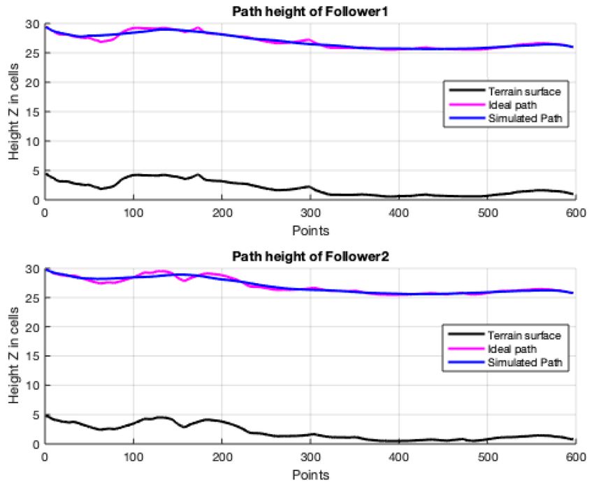
Drones 2023, 7, 84                                                                                             3 of 18

                     Figure 2. Data fitted to a Gaussian Mixture model.

                          Once the search area is well defined, the trajectory to conveniently reach its full breadth
                     must be designed. This task is widely known as coverage. Researchers in the literature
                     distinguish two different approaches, namely [15]: lawnmower algorithms and control of
                     the agents through optimization processes.
                          In a lawnmower strategy, search agents will sweep the target area by going back and
                     forth following a specific pattern. These patterns are conveniently designed to find the
                     target in shorter time. Figure 3 shows different patterns proposed by authors working on
                     the matter. What makes this strategy interesting is that, just on the basis of these primitive
                     patterns and adding some custom design criteria, good results can be obtained for a low
                     computational cost.

                     Figure 3. Different search patterns for search and rescue [16].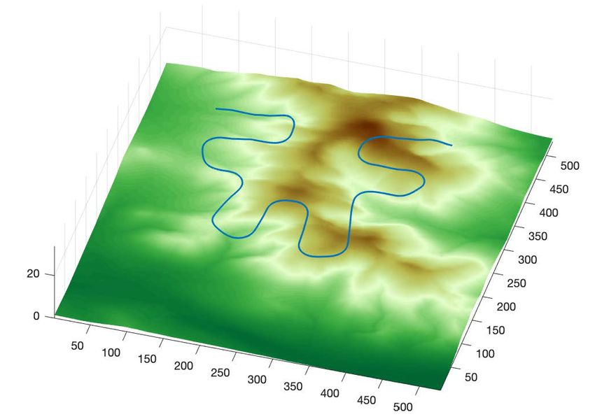
Drones 2023, 7, 84                                                                                           4 of 18

                           Researchers in [17] use this approach to study and improve the calculation method
                     of the aforementioned probability of containment measure, as well as the probability of
                     detection and thus the probability of success values. This probability of detection is mainly
                     related to the efficiency of the path designed and available sensors to cover the full search
                     area and therefore detect the targets. Then, the probability of coverage success would
                     depend on these other factors.
                           One could look at this path planning task as an optimization problem. Then, the goal
                     would be to compute this search trajectory by minimizing a certain performance met-
                     ric that may be related to, for instance: fuel consumption, travel times, path length or,
                     as in the well-known salesman problem, visiting all target areas (if more than one exists)
                     just once while following the shortest path. This issue is commonly addressed through
                     swarm optimization algorithms, as its aim is to provide ’best locations’ within a search
                     space using swarms [18–20]. Particle Swarm Optimization is notably highlighted in the
                     literature from this whole family of algorithms [21,22]. For its part, authors in [23] study
                     the problem of dynamically covering a given region through a designed closed-loop control
                     strategy. Their goal was to provide, for each target point of the domain, a certain amount
                     of effective coverage.
                           Finally, once the coverage problem has been formulated, it seems interesting to un-
                     derline that most of these tasks are usually carried out not just by a single search vehicle
                     but by a swarm, following a specific formation or not [24]. Multirobot (or multivehicle)
                     systems have certain advantages over single-robot missions. Several tasks can be executed
                     in parallel, provide a wider sensing range and the whole system can be more robust to
                     failures of one of the vehicles [20,25–29]. Regarding this topic, our group has worked on the
                     robot formations planning problem (both in 2D and 3D) using the Fast Marching Square
                     (FM2 ) algorithm [30,31].
                           In this work, we are going to study the coverage and robot formation problems,
                     introducing probability maps and implementing the FM2 algorithm, in two closely re-
                     lated situations. The first aimed at search missions in mountain areas using Unmanned
                     Autonomous Vehicle (UAV) formations and the latter focusing on maritime search tasks
                     carried out by an Unmanned Autonomous System (UAS).
                           The main contributions of this paper are: (1) a simple approach lawnmower strategy
                     is presented to face the coverage path planning problem for search and rescue tasks carried
                     out by UAVs in different 3D environments; (2) the coverage method is based on the use
                     of Gaussian Mixture to approximate the probability of containment distribution, Voronoi
                     Diagrams to skeletonize the Gaussian Mixture, geometric generation of the lawnmower
                     zigzag coverage path and Fast Marching Square to obtain smooth, optimal in terms of
                     distance cost and collision free trajectories; (3) the method is extended to UAV team
                     formations and the strategy is usable for different swarm configurations and numbers of
                     team vehicle members; (4) the search environments aimed at this work may present diverse
                     shapes and may be composed of a single compact target zone or a series of disjoint areas;
                     (5) the target zones may constitute uneven ground terrain levels and the flight height at
                     which the coverage mission is planned can be chosen at will and is relative to this varying
                     ground level.
                           The rest of the paper is organized as follows. Section 2 describes the Eikonal Equation
                     and the Fast Marching Method. Section 3 introduces the Coverage Path Planning carried
                     out by a single UAV and also presents the UAVs formation approach. Section 4 shows the
                     results from two cases of application. Finally, in Section 5, the main conclusions of the work
                     are presented.

                     2. The Fast Marching Method
                          The Fast Marching method was proposed by J.A. Sethian in 1996 [32]. This method lead
                     to an extremely fast scheme to solve the eikonal equation in Cartesian grids. The eikonal
                     equation models the propagation of an isometric wave front. Rays of light, traveling
                     through different materials, follow the least time-consuming path, according to Fermat’s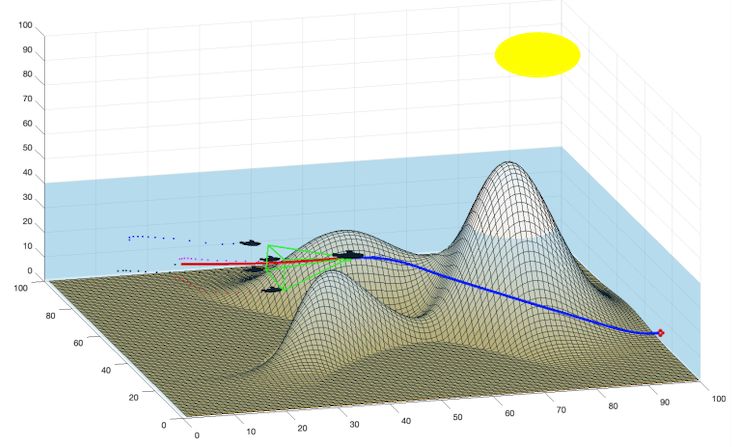
Drones 2023, 7, 84                                                                                            5 of 18

                     principle [33]. This is an interest concept in robotics due to the fact that, if we know how
                     light rays propagate through space, we can calculate the trajectory between two points of a
                     map. This trajectory can be obtained with the Fast Marching method (FMM).
                           If we consider the target point of a trajectory as the source of a light wave front,
                     and the Fast Marching method can be computed over the free cells of a map, the arrival
                     time of the wave front to each point of the map is calculated. Furthermore, taking the set
                     of all cells that represent the free space and the time of arrival to those cells into account,
                     a Lyapunov surface in which all level curves are isochronous can be created, and the
                     Lyapunov trajectories are orthogonal to said curves. This means that it is not possible for
                     the method to show local minima. An example of this surface can be seen in Figure 4.

                     Figure 4. Funnel potential obtained when using the time of arrival as the third axis.

                          The propagation of the light wave front is given by the eikonal Equation (1). Sethian [32]
                     proposed a first order approximation to this equation and called it FMM. The eikonal equa-
                     tion defines the time of arrival of the propagating wavefront, T ( x ), to every point x,
                     in which the wave front propagation speed depends on the point F ( x ), according to:

                                                     |∇ T ( X )| F ( x ) = 1, x ⊂ R N                            (1)
                           The Fast Marching method consists of solving the Equation (1) and calculate sequen-
                     tially T ( x ) for every cell of the map starting from the wave source point where T ( xo ) = 0.
                     After using FMM, gradient descent can be used from any distance map point to obtain a
                     path to the wave source as a target point. The main advantage of this approach is that the
                     resulting paths are time optimal. An example of a path generated using FMM and another
                     calculated using FM2 is shown in Figure 5.

                                           (a)                                               (b)

                     Figure 5. Comparison between a path generated with (a) FMM and another generated with (b) FM2 .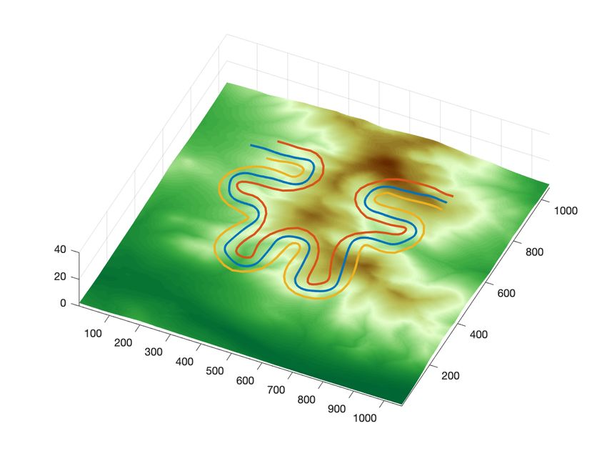
Drones 2023, 7, 84                                                                                                6 of 18

                     The Fast Marching Square Method
                          As it can be seen in Figure 6a, although optimal in distance, the trajectory is neither
                     safe in terms of possible collision with obstacles nor feasible in terms of the sharpness of
                     the turns the trajectory requires. These series of disadvantages lead to study the use of the
                     Fast Marching Square method (FM2 ) [34] as a path planner, since it gives a solution to these
                     two disadvantages. It consists of applying FMM two times as shown in Figure 5b.
                          Let us consider a map in which obstacles take the value 1 and free cells take the value
                     0. FMM can be applied to these map considering all obstacles as wave sources. An example
                     of this method is shown in Figure 6.

                     Figure 6. Application of the FM2 method. From left to right: the original map, the speed map in
                     which the maximum value is saturated, the time of arrival map as a result of the wave expansion and
                     the resulting path in the initial map.

                          This map can be explained in many ways. It can be interpreted as a potential field of
                     the original map, as cells move away from obstacles, the Ti value gets higher, like in the
                     case of the distances map. Furthermore, it can be seen as a velocity map: the Ti value can
                     be interpreted proportional to the maximum speed achievable for the robot in each point,
                     which leads to permitting lower speeds when the point is close to an obstacle, and higher
                     speeds when it is away from them. In fact, a robot which speed in each point is given by Ti
                     will never collide with obstacles, since Ti → 0 as it gets closer to an obstacle. Further into
                     this work, this first potential is referred to as potential W.
                          The second time the FMM is applied (obtaining potential D), the velocity at which the
                     wave front advances can be different in each point of the map. Furthermore, this velocity
                     is proportional to the distance to the closest obstacle, which means that the wave front
                     advances faster when it is away from obstacles. This produces important differences in the
                     trajectory obtained, as it can be seen in Figure 4. The final trajectory is obtained through
                     gradient descent methods, as for the original FMM.
                          The FM2 method has some properties that make it really useful to plan trajectories.
                     The most important advantages are:
                     •    No local minima.
                     •    Complete.
                     •    Smooth trajectories.
                     •    Fast response with O(n) complexity [35].

                     3. Problem Statement
                     3.1. Coverage Path Planning of the Leader of the UAVs Formation
                           As it has been previously mentioned, the method presented in this paper for Coverage
                     Path Planning (CPP) aims to be applied to UAV formations. In this way, the strategy is
                     first defined for the leader of the UAV formation team. The technique used belongs to the
                     aforementioned lawnmower family of coverage planning algorithms, sufficiently optimized
                     to be both efficient and easy to implement.
                           The 3D environment where the path planning for covering with a UAVs formation is
                     carried out is the terrain height near Mount Washington as a function of x–y position (In
                     this case, Mount Washington is the highest peak in the northeastern United States.)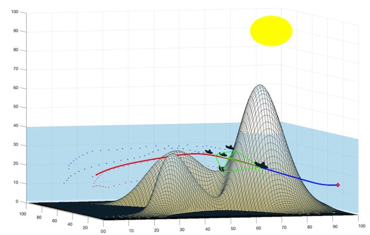
Drones 2023, 7, 84                                                                                                  7 of 18

                           The US Geological Survey provides terrain elevation data as a function of x–y position
                     on the grid. To estimate the height of an arbitrary point, the objective function interpolates
                     the height from nearby grid points.
                           The 3D grid map has a dimension of 550 × 550 × 40 cells, where each cell of the map
                     is equivalent to 15 × 15 × 15 m. It is not necessary to consider the sizes of the UAVs, since
                     it is assumed tobe smaller than the size of a cell. In Figures 7 and 8, the grid map has a
                     dimension of 750 × 750 × 40 cells to have a denser coverage.

                                            (a)                                               (b)

                     Figure 7. (a) FM2 second potential expansion at a certain level (25), and (b) smooth 3D path obtained
                     by computing the geodesic in the D expansion for a denser coverage and with more resolution
                     (750 × 750 cells).

                     Figure 8. Final smooth path obtained with FM2 for a denser coverage and with more resolution
                     (750 × 750 cells).

                          The procedure is detailed below.
                          This method is based in the Gaussian Mixture approximation of the probability of
                     containment density function that defines the searching area, which is assumed to be
                     already characterized. The method is composed by the following steps:
                     1.    Find the Gaussian Mixture that approximates the probability function given. In this
                           manner, the domain is simplified to a series of Gaussian distributions, and it is possible
                           to apply the upcoming steps to the Gaussians. Figures 9a and 7a shows a search region
                           given by three Gaussians.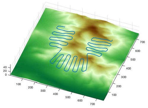
Drones 2023, 7, 84                                                                                             8 of 18

                     2.    Identify the minimum level of probability to find the area to be covered. This zone
                           can be compact or composed by different unconnected zones, as shown in Figure 7a.
                     3.    Using the Voronoi method, the medial axis of the zones is calculated. The medial axis
                           may be a curve or can be made up of unconnected sections. For isolated Gaussians,
                           the medial axis is the main axis of the Gaussian. For nonisolated Gaussians, the medial
                           axis is a curve composed by the points that are at the same distance to the borders of
                           the probability threshold.
                     4.    The next step is to find the points that divide the medial axis into segments of the
                           same length.
                     5.    The line segments perpendicular to the medial axis that pass through these points are
                           calculated. The segments end where the chosen probability threshold is reached.
                     6.    The ends of these segments are joined alternately to obtain a complete zigzag path.
                           This is done optimally so that the overall length is minimized. Figure 9b shows a 2D
                           zigzag path composed by segments obtained this way.
                     7.    Heights are added so that the path becomes a three-dimensional path. Figure 10a
                           shows a 3D path obtained by adding the desired height above the ground to the
                           previous path. It is important to notice that the ground terrain level may be irregular.
                     8.    As it is not smooth enough, a three-dimensional tube is calculated through image
                           processing techniques, dilating the path as shown in Figure 10b.
                     9.    The first Fast Marching potential W is calculated inside the tube so that the path tends
                           to go through the middle of the tube smoothly.
                     10.   On this first potential W, the second potential D is calculated from the end point. This
                           process finishes when the expansion wave reaches the start point. A slice at a certain
                           height of this D expansion is shown in Figure 11a.
                     11.   On this potential D, the 3D geodesic path is calculated, from the initial point to the
                           goal point using the gradient descend method. Figure 11b shows the final smooth
                           path obtained with this process.
                     12.   Final smooth path over the terrain surface is shown in Figure 12, whereas
                           Figure 13 shows a lateral view of this terrain surface (in black), ideal path (in magenta)
                           and smooth path obtained with FM2 (in blue).

                                       (a)                                            (b)

                     Figure 9. (a) Search region given by three Gaussians, and (b) 2D path composed by segments.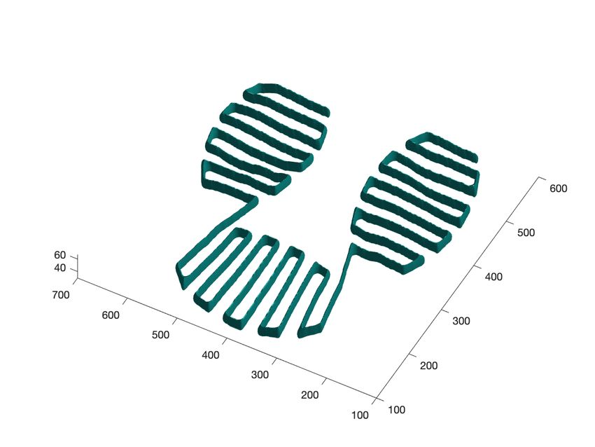
Drones 2023, 7, 84                                                                                                   9 of 18

                                              (a)                                            (b)

                     Figure 10. (a) 3D path obtained by adding the desired height above the ground, and (b) tube around
                     the previous path.

                                        (a)                                               (b)

                     Figure 11. (a) FM2 second potential expansion at a certain level (25), and (b) smooth 3D path obtained
                     by computing the geodesic in the D expansion.

                     Figure 12. Final smooth path obtained with FM2 .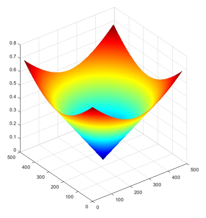
Drones 2023, 7, 84                                                                                               10 of 18

                     Figure 13. Terrain surface (in black), ideal path (in magenta), and smoothed path obtained with FM2
                     (in blue).

                     3.2. UAVs Formation Algorithm
                          The previous subsection shows how to find out the path for a UAV that will constitute
                     the path of the leader of the formation. Now, it is necessary to explain how, from this
                     path, the trajectories for every UAV in the formation are calculated, taking the possible
                     irregularities of the terrain and the obstacles present in the environment into account.
                          Suppose a triangular formation, with a leading UAV and two followers. The other
                     possible formations would be treated in a similar way. The formation consists of a first
                     pure geometric triangular shape (magenta triangle in Figure 14) that is deformed according
                     to the needs to avoid the obstacles that appear on the route and the path itself by using
                     the gray levels. This second deformed triangle is the one that UAVs must follow (magenta
                     triangle in Figure 14).
                          This second deformed triangle is calculated using the remaining vehicles as obstacles.
                     Using the gray level potential present in the Fast Marching method as shown in Figure 15,
                     each UAV sees the rest of the UAV’s as obstacles in the environment. This effect provides
                     additional repulsion force, preventing them from colliding with the other UAVs.
                          Thus, the stages for planning the trajectory for a whole UAV team flying in formation
                     are detailed hereinafter. The different steps to obtain the trajectory of the leader are:
                     1.   We start with a binary map Wo of zeros (black area represents the obstacles) and ones
                          (white area represents the zone without obstacles) as shown in Figure 14a.
                     2.   The Fast Marching method is applied to this binary map Wo, taking obstacles as wave
                          origin points. In this way, a gray map W is obtained, in which the grayscale level
                          represents the distance to the nearest obstacle. You can also do this step using the
                          Voromoi Transform, although the performance is not that good due to its discrete
                          nature. This map can be considered as the map of relative speeds of expansion of the
                          wave and also of the leader. (grey potential in Figure 14b,c).
                     3.   On this first potential W, a wave is launched from the destination point, again using
                          the Fast Marching method, to the origin point. This gives us the second funnel-shaped
                          potential D (color potential in Figure 14d).
                     4.   The gradient descent method is applied to D second potential to find the minimum
                          time path. The generated path is the trajectory that the leader must follow.
                          The distance between the lines of the zigzag can be changed to have a denser coverage
                     of the zone as shown in Figures 7 and 8 and with more resolution (750 × 750 cells).
                          As for this work, the trajectory corresponding to the leader is computed following
                     the steps described in Section 3.1. Then, when the path of the leader has been generated,
                     the paths of the followers are calculated iteratively. In each cycle of time t and for each
                     U AV, referred to as U AVi , a partial goal and a partial path are calculated that will continue
                     until the next cycle. The iterations t are calculated in the following way:
                     1.   Each U AVi is associated with a binary map W t0,i which acts as obstacle map, with the
                          leader and the other followers considered as obstacles. Figure 14a represents the
                          binary map W t0,i with the obstacles and the others UAV’s of the formation in black
                          (value 0) and the allowed parts are white (value 1).
                     2.   For each UAVi , a new first grayscale potential Wit is generated from the binary map
                          W t0,i in each cycle t by using FMM the first time, using all black points as starting
                          points and obtaining the first potential of wave expansion velocities. Figure 14b
Drones 2023, 7, 84 11 of 18
shows the grayscale map Wit of the right follower obtained from the corresponding
binary map W0,i t with two blurred black dots representing the leader and the left
follower. In Figure 14c, is shown the grayscale map Wit corresponding to the leader ob-
tained from the initial binary map W0,i t , with two blurred black spots representing the
two followers.
3. The subgoals Pt (x g,i , y g,i , z g,i ) for each follower are calculated based on the leader’s
position of the previous FM2 leader trajectory. These partial targets indicate the next
desired goal for each follower and form the deformable geometric triangle as shown
in Figure 8 (magenta triangle). Obstacles in the environment (including other drones)
are taken into account when calculating this position. For this purpose, the grayscale
level of each subtarget goal is calculated from Wit , which conveniently changes the
triangle distances (edges and vertices). This approach introduces a repulsive force
against obstacles and the other UAVs in the environment. More details can be seen
in [36].
Figure 14. UAVs formation algorithm: (a) leader and followers with its partial goals; (b) deformable
geometrical triangle (in blue) and real positions triangle (in magenta) of UAV formation; (c) modi-
fication of the partial goals of the followers according to the leader position in a curved trajectory;
(d) modification of partial goals according to the obstacles of the environment.Drones 2023, 7, 84 12 of 18
(a) (b)
(c) (d)
Figure 15. UAVs formation approach: (a) UAVs formation following their corresponding paths;
(b) first grayscale potential map W of the right follower taking the leader and the left follower as
blurred obstacles; (c) first grayscale potential map W of the leader taking the followers as obstacles;
(d) second potential map D of the leader taking the followers as obstacles.
Figure 16 shows the trajectories of the followers in (a) XY view and (b) the trajectories
followed by the UAVs, whereas Figure 17 shows the trajectories of leader and followers
over the terrain surface.Drones 2023, 7, 84 13 of 18
(a) (b)
Figure 16. Trajectoriesof the followers in (a) XY view and (b) the trajectories followed by the UAVs.
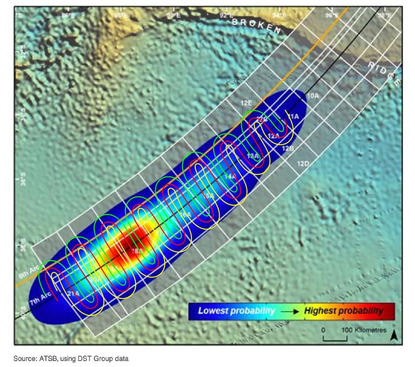
In the previous CPP example presented for a mountainous area, the Gaussians were
disjoint and the medial axis coincides with the main axis of the ellipse, but when the
Gaussian mixture is not composed of disjoint distributions, the medial axis is not a series of
straight segments. For example, Figure 17 shows the probability function of the search zone
of the accident of the Malaysia Airlines Flight MH370 with the three paths of the UAV’s
formation. In this case, the medial axis is a curved line.
Figure 17. Trajectories of leader and the followers above the terrain.
4. Results
As can be seen in the figures above, the paths of each member of the formation are
smooth, and the trajectories are safe to be followed by real UAVs. The difference is that
the trajectories calculated with FMM have sudden changes of direction and collide with
the obstacles while the trajectories obtained with FM2 are smooth and move away from
the obstacles. With the word smooth, we mean that the continuous solution has all the
derivatives, that is, it is of class C ∞ . In our case, we have a discrete solution that depends on
the size of the grid, and when it tends to zero, the discrete solution tends to the continuousDrones 2023, 7, 84 14 of 18
C ∞ solution. The practical meaning is that this type of trajectory can be easily followed by
a UAV.
In Figure 18, it can be seen that the method also works to make a covering in other
probability spots such as the accident of the Malaysia Airlines Flight MH370. In Figure 7,
the height relative to the ground of the leader is shown, which follows the desired values.
Those of the followers are similar, as can be seen in Figure 19. The simulation results
show that the formation is able to adapt its shape to avoid obstacles while respecting flight
level constraints.
Likewise, Figures 17 and 20 shows that the distances among the three members of
the formation are correct, because the geometric triangle is deformable but has a range of
action so that they do not become too close. As can be seen, the distance minimum among
the UAVs formation members is bigger than 50 cells.
As the gray level potential of the first step of the calculation of FM2 represents the
relative velocity between 0 and 1, we have the recommended relative velocity for each
member of the formation in each point, as shown in Figure 21. If this relative velocity is
multiplied by the maximum velocity of the UAVs measured in cells per iteration, the real
velocity of the three UAVs in cells/iterations is obtained as shown in Figure 22.
The method can be applied to other formations and scenarios. As an example, Figure 23
represents the approach for the case of a leader ship followed by four mini-submarines in a
pyramid formation.
Figure 18. Probability function of the search zone of the accident of the Malaysia Airlines Flight
MH370 with the three paths of the UAV’s formation.Drones 2023, 7, 84 15 of 18
Figure 19. Trajectories of the followers above the terrain. Terrain surface (in black), ideal path (in
magenta), and smoothed path obtained with FM2 (in blue).
Figure 20. Internal distances among the three members of the formation.
Figure 21. Recommended velocity, between 0 and 1, of the three UAVs using gray level potential.Drones 2023, 7, 84 16 of 18
Figure 22. Real velocity of the three UAVs in cells/iterations.
(a) (b)
Figure 23. Other possible formations and other scenarios: a ship followed by four mini-submarines
in a pyramid formation (a,b).
5. Conclusions
In this work, we present a new technique to solve the probabilistic Coverage Path
Planning (CPP) problem for search and rescue by a formation of UAVs based on Gaussian
Mixture to approximate the probability distribution, Voronoi Diagram for the skeletoniza-
tion of the Gaussian mixture, geometric generation of a zigzag path and finally the Fast
Marching Square method (FM2 ) a feasible path free from obstacles for the UAV’s formation
that maintains a flight level with respect to the ground. The generated path is optimal not
only in terms of distance cost but also in terms of safety and smoothness and, therefore,
feasible for the UAV.
One of the advantages of the FM2 Method is its flexibility, because by conveniently
modifying the first potential (first step of FM2 ), it is possible to obtain the desired path
properties and trajectories that can be easily followed by UAVs.
Our approach has proved successful. The tests carried out show good results, even on
uneven terrain, always achieving a feasible path with minimum cost. This result shows
that our method generates paths that conserve energy or fuel and, furthermore, trajectories
that are safe and compatible with UAV kinematics.
In further research, other formations, in different scenarios and in real situations can
be studied.
Author Contributions: Conceptualization by S.G., C.A.M., L.M.; methodology design by S.G. and
C.A.M.; software by J.M.; validation by B.L.; formal analysis by F.Q.; project administration by C.A.M.
All authors have read and agreed to the published version of the manuscript.Drones 2023, 7, 84 17 of 18
Funding: The research leading to these results has received funding from the “EUROPEAN COM-
MISSION Innovation and Networks Executive Agency. Project number 861696-LABYRINTH”.
Data Availability Statement: Not applicable.
Conflicts of Interest: The authors declare no conflict of interest.
References
1. Ghazali, S.N.A.M.; Anuar, H.A.; Zakaria, S.N.A.S.; Yusoff, Z. Determining position of target subjects in Maritime Search and
Rescue (MSAR) operations using rotary wing Unmanned Aerial Vehicles (UAVs). In Proceedings of the 2016 International
Conference on Information and Communication Technology (ICICTM), Kuala Lumpur, Malaysia, 16–17 May 2016; IEEE: New
York, NY, USA , 2016; pp. 1–4.
2. Abi-Zeid, I.; Nilo, O.; Lamontagne, L. A constraint optimization approach for the allocation of multiple search units in search and
rescue operations. Inf. Inf. Syst. Oper. Res. 2011, 49, 15–30.
3. Australian Transport Safety Bureau. The Operational Search for MH370. Canberra, Australian Capital Territory, Commonwealth of
Australia; Technical Report AE-2014-054; Australian Transport Safety Bureau: Canberra, Australia, 2017.
4. Yilmaz, A.; Javed, O.; Shah, M. Object tracking: A survey. Acm Comput. Surv. (CSUR) 2006, 38, 13-es. [CrossRef]
5. Ward, S.; Hensler, J.; Alsalam, B.; Gonzalez, L.F. Autonomous UAVs wildlife detection using thermal imaging, predictive
navigation and computer vision. In Proceedings of the 2016 IEEE Aerospace Conference, Big Sky, MT, USA, 5–12 March 2016;
pp. 1–8.
6. Chen, D.; Liu, Z.; Wang, L.; Dou, M.; Chen, J.; Li, H. Natural Disaster Monitoring with Wireless Sensor Networks: A Case Study
of Data-intensive Applications upon Low-Cost Scalable Systems. Mob. Netw. Appl. 2013, 18, 651–663. [CrossRef]
7. Ho, D.-T.; Grøtli, E.I.; Sujit, P.B.; Johansen, T.A.; Sousa, J.B. Optimization of Wireless Sensor Network and UAV Data Acquisition.
J. Intell. Robot. Syst. 2015, 78, 159–179.
8. Ko, A.; Lau, H.Y. Robot assisted emergency search and rescue system with a wireless sensor network. Int. J. Adv. Sci. Technol.
2009, 3, 69–78.
9. Alotaibi, E.T.; Alqefari, S.S.; Koubaa, A. LSAR: Multi-UAV Collaboration for Search and Rescue Missions. IEEE Access 2019, 7,
55817–55832. [CrossRef]
10. Kim, M.-H.; Baik, H.; Lee, S. Response Threshold Model Based UAV Search Planning and Task Allocation. J. Intell. Robot. Syst.
2014, 75, 625–640. [CrossRef]
11. Di Franco, C.; Buttazzo, G. Energy-aware coverage path planning of UAVs. In Proceedings of the 2015 IEEE international
conference on autonomous robot systems and competitions, Vila Real, Portugal, 9–10 April 2015; pp. 111–117.
12. Galceran, E.; Carreras, M. A survey on coverage path planning for robotics. Robot. Auton. Syst. 2013, 61, 1258–1276. [CrossRef]
13. Ivić, S.; Crnković, B.; Arbabi, H.; Loire, S.; Clary, P.; Mezić, I. Search strategy in a complex and dynamic environment: The
MH370 case. Sci. Rep. 2020, 10, 1–15.
14. Reynolds, D.A. Gaussian Mixture Models. Encycl. Biom. 2009, 741, 659–663.
15. Mathew, G.; Mezić, I. Metrics for ergodicity and design of ergodic dynamics for multi-agent systems. Phys. Nonlinear Phenom.
2011, 240, 432–442.
16. Guoxiang, L.; Maofeng, L. Sargis: A gis-based decision-making support system for maritime search and rescue. In Proceedings of
the 2010 International Conference on E-Business and E-Government, Guangzhou, China, 7–9 May 2010; pp. 1571–1574.
17. Agbissoh, O.D.; Li, B.; Ai, B.; Gao, S.; Xu, J.; Chen, X.; Lv, G. A decision-making algorithm for maritime search and rescue plan.
Sustainability 2019, 11, 2084. [CrossRef]
18. Parker, L.E. Decision making as optimization in multi-robot teams. In Proceedings of the International Conference on Distributed
Computing and Internet Technology, Bhubaneswar, India, 2–4 February 2012; Springer: Berlin/Heidelberg, Germany, 2012;
pp. 35–49.
19. Senanayake, M.; Senthooran, I.; Barca, J.C.; Chung, H.; Kamruzzaman, J.; Murshed, M. Search and tracking algorithms for swarms
of robots: A survey. Robot. Auton. Syst. 2016, 75, 422–434. [CrossRef]
20. Phung, M.D.; Ha, Q.P. Safety-enhanced UAV path planning with spherical vector-based particle swarm optimization. Appl. Soft
Comput. 2021, 107, 107376. [CrossRef]
21. Pugh, J.; Martinoli, A. Inspiring and modeling multi-robot search with particle swarm optimization. In Proceedings of the
2007 IEEE Swarm Intelligence Symposium, Honolulu, HI, USA, 1–5 April 2007; pp. 332–339.
22. Wang, Y.; Bai, P.; Liang, X.; Wang, W.; Zhang, J.; Fu, Q. Reconnaissance Mission Conducted by UAV Swarms Based on Distributed
PSO Path Planning Algorithms. IEEE Access 2019, 7, 105086–105099.
23. Hussein, I.I.; Stipanovic, D.M. Effective Coverage Control for Mobile Sensor Networks With Guaranteed Collision Avoidance.
IEEE Trans. Control. Syst. Technol. 2007, 15, 642–657.
24. Arkin, R.C.; Arkin, R.C. Behavior-Based Robotics; MIT Press: Cambridge, MA, USA, 1998.
25. Oubbati, O.S.; Lakas, A.; Lorenz, P.; Atiquzzaman, M.; Jamalipour, A. Leveraging Communicating UAVs for Emergency Vehicle
Guidance in Urban Areas. IEEE Trans. Emerg. Top. Comput. 2019, 9, 1070–1082.
26. Krátký, V.; Alcántara, A.; Capitán, J.; Štěpán, P.; Saska, M.; Ollero, A. Autonomous aerial filming with distributed lighting by a
team of unmanned aerial vehicles. IEEE Robot. Autom. Lett. 2021, 6, 7580–7587.Drones 2023, 7, 84 18 of 18
27. Spurný, V.; Báča, T.; Saska, M.; Pěnička, R.; Krajník, T.; Thomas, J.; Thakur, D.; Loianno, G.; Kumar, V. Cooperative autonomous
search, grasping, and delivering in a treasure hunt scenario by a team of unmanned aerial vehicles. J. Field Robot. 2019, 36,
125–148. [CrossRef]
28. Liu, H.; Lyu, Y.; Zhao, W. Robust visual servoing formation tracking control for quadrotor UAV team. Aerosp. Sci. Technol. 2020,
106, 106061. [CrossRef]
29. Moon, H.; Martinez-Carranza, J.; Cieslewski, T.; Faessler, M.; Falanga, D.; Simovic, A.; Scaramuzza, D.; Li, S.; Ozo, M.; De Wagter,
C.; et al. Challenges and implemented technologies used in autonomous drone racing. Intell. Serv. Robot. 2019, 12, 137–148.
[CrossRef]
30. Gómez, J.V.; Lumbier, A.; Garrido, S.; Moreno, L. Planning robot formations with fast marching square including uncertainty
conditions. Robot. Auton. Syst. 2013, 61, 137–152. [CrossRef]
31. Alvarez, D.; Gómez, J.V.; Garrido, S.; Moreno, L. 3D robot formations path planning with fast marching square. J. Intell. Robot.
Syst. 2015, 80, 507–523.
32. Sethian, J. A fast marching level set method for monotonically advancing fronts. Proc. Natl. Acad. Sci. USA 1996, 93, 1591–1595.
[CrossRef] [PubMed]
33. Born, M.; Wolf, E. Principles of Optics: Electromagnetic Theory of Propagation, Interference and Diffraction of Light; Elsevier: Amsterdam,
The Netherlands, 2013.
34. Garrido, S.; Moreno, L.; Abderrahim, M.; Blanco, D. FM2: A real-time sensor-based feedback controller for mobile robots. Int.
Robot. Autom. 2009, 24, 3169–3192.
35. Yatziv, L.; Bartesaghi, A.; Sapiro, G. O (N) implementation of the fast marching algorithm. J. Comput. Phys. 2006, 212, 393–399.
[CrossRef]
36. Monje, C.A.; Garrido, S.; Moreno, L.; Balaguer, C. UAVs Formation Approach Using Fast Marching Square Methods. IEEE Aerosp.
Electron. Syst. Mag. 2020, 35, 36–46. [CrossRef]
Disclaimer/Publisher’s Note: The statements, opinions and data contained in all publications are solely those of the individual
author(s) and contributor(s) and not of MDPI and/or the editor(s). MDPI and/or the editor(s) disclaim responsibility for any injury to
people or property resulting from any ideas, methods, instructions or products referred to in the content.You can also read