FACS-Based Proteomics Enables Profiling of Proteins in Rare Cell Populations - MDPI
←
→
Page content transcription
If your browser does not render page correctly, please read the page content below
International Journal of
            Molecular Sciences

Article
FACS-Based Proteomics Enables Profiling of Proteins
in Rare Cell Populations
Evelyne Maes 1 , Nathalie Cools 2,3 , Hanny Willems 4,5 and Geert Baggerman 4,5, *
 1    Food & Bio-Based Products, AgResearch Ltd., Lincoln 7674, New Zealand; Evelyne.Maes@agresearch.co.nz
 2    Laboratory of Experimental Hematology, Faculty of Medicine and Health Sciences, Vaccine and Infectious
      Disease Institute (VaxInfectio), Antwerp University Hospital (UZA), University of Antwerp,
      2020 Antwerpen, Belgium; Nathalie.Cools@uza.be
 3    Center for Cell Therapy and Regenerative Medicine, Antwerp University Hospital, 2650 Edegem, Belgium
 4    Centre for Proteomics, University of Antwerp, Groenenborgerlaan 171, 2020 Antwerpen, Belgium;
      hanny.willems@vito.be
 5    Health Unit, Vlaamse Instelling voor Technologisch Onderzoek (VITO), Boeretang 200, 2400 Mol, Belgium
 *    Correspondence: Geert.Baggerman@vito.be; Tel.: +32-476472918

 Received: 27 July 2020; Accepted: 4 September 2020; Published: 8 September 2020

 Abstract: Understanding disease pathology often does not require an overall proteomic analysis
 of clinical samples but rather the analysis of different, often rare, subpopulations of cells in a
 heterogeneous mixture of cell types. For the isolation of pre-specified cellular subtypes, fluorescence
 activated cell sorting (FACS) is commonly used for its ability to isolate the required cell populations
 with high purity, even of scarce cell types. The proteomic analysis of a limited number of FACS-sorted
 cells, however, is very challenging as both sample preparation inefficiencies and limits in terms of
 instrument sensitivity are present. In this study, we used CD14+CD15+ immune cells sorted out of
 peripheral blood mononuclear cells isolated from whole blood to improve and evaluate FACS-based
 proteomics. To optimize both the protein extraction protocol and the mass spectrometry (MS) data
 acquisition method, PBMCs as well as commercialized HeLa digest were used. To reflect the limited
 number of sorted cells in some clinical samples, different numbers of sorted cells (1000, 5000, 10,000,
 or 50,000) were used. This allowed comparing protein profiles across samples with limited protein
 material and provided further insights in the benefits and limitations of using a very limited numbers
 of cells.

 Keywords: FACS; proteomics; cellular heterogeneity

1. Introduction
     The cellular heterogeneity of human clinical samples represents a major challenge for clinical
proteomics, as in many cases the results achieved by the analysis of undefined cell populations might
be misleading. In many biomedical and clinical proteomics experiments, for example, the entire
tissue of interest is homogenized or tissue slices are processed resulting in an ‘average’ cellular
response. These approaches might deliver valuable information but do not allow obtaining molecular
information associated with certain cellular subpopulations of interest or diluting relevant effects on
protein expression of distinct cell populations in the overall background below the detection limit.
In many research questions, the prefractionation of specific cell types is therefore desirable. These days,
a wide range of cell isolation techniques are available, with density gradient centrifugation, cell filtering,
and immunoaffinity methods as most prominent. Although density gradients are frequently used
for the separation of plasma, platelets, peripheral blood mononuclear cells (PBMCs) or erythrocytes
from other blood constituents [1], immunoaffinity techniques can be used in both liquid and tissue

Int. J. Mol. Sci. 2020, 21, 6557; doi:10.3390/ijms21186557                          www.mdpi.com/journal/ijms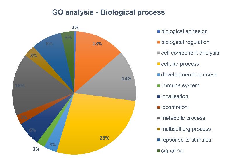
Int. J. Mol. Sci. 2020, 21, 6557                                                                      2 of 12

biopsies and enable enrichment of a wide variety of cell types and organelles [2,3]. This immune-based
enrichment of specific cell types is based on antibodies, and their isolation from human in vivo
specimens is thus limited to cell populations that have distinct surface markers [4]. The isolation of
specific cell types is these days commonly performed by means of flow cytometry. In flow cytometry
and fluorescence activated cell sorting (FACS), the heterogenous cell population from a tissue or
liquid biopsy is placed in suspension, all particles (including the living cells) are placed in a fluid
stream, enter the flow cell in a cell-by-cell way through a nozzle, pass by a set of lasers, and the light
scattering and fluorescence signals of each particle passing by are detected. Based on user-defined
settings, individual cells can then be collected into homogeneous fractions [5]. This way, FACS can
sort cells based on specific, user-defined light scattering and fluorescent characteristics of each cell
type and allow the enrichment of even low abundant subpopulations, with high purity. In addition to
fluorescent-based cell sorting, enrichment is also possible by means of magnetic activated cell sorting
(MACS). In MACS, small paramagnetic beads, instead of fluorescent tags, are coupled to the antibodies,
which allows isolation of cells of interest using specialized magnets. Compared to FACS, MACS has
the major advantage of ease-of-use [6]. On the other hand, FACS is by definition a cell-by-cell analysis,
while MACS analysis is more of a bulk analysis. Therefore, typically, a higher purity of the desired cell
population is achieved by FACS. Regardless of the obtained purity, both FACS and MACS can be used
to deplete unwanted cells (negative sorting) or to isolate target cell types (positive sorting).
      Proteomics analysis of prespecified cell populations can deliver insights into cell-specific
functionalities, which is often essential to obtain more knowledge about their specific role. The restricted
amounts of in vivo sourced material (e.g., tissue biopsies) combined with the overall cell heterogeneity,
however, complicates the overall proteomics procedure as the number of FACS-enriched cells from
in vivo samples is often very limited (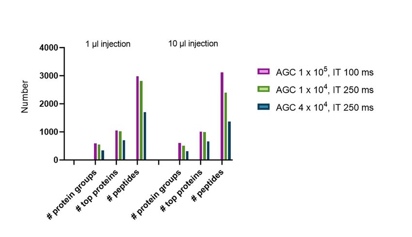
Int. J. Mol. Sci. 2020, 21, 6557 3 of 12
Int. J. Mol. Sci. 2020, 21, x FOR PEER REVIEW 3 of 12
commonly used in proteomics, could not minimize the effect of the non-MS compatible contaminants
in the
thesamples.
samples.AnAn additional
additional precipitation
precipitation withwith ice-cold
ice-cold (−80 ◦ C),
acetone
acetone (−80however,
°C), however,
was verywas very
effective
effective
to reducetothe
reduce
levelthe level of contamination
of contamination (i.e., loosing/lowering
(i.e., loosing/lowering the ionsthe ions linked
linked to the sheath
to the sheath flow offlow
the
of the FACS
FACS instrument)
instrument) to such
to such an extent
an extent thatthat peptides
peptides and and proteins
proteins couldbebeidentified
could identifiedand
and nono major
chromatographic peaks containing singly charged ions could could be
be detected.
detected.
2.2. Peptide
2.2. Peptide Separation
Separation and
and Mass
Mass Spectrometry
Spectrometry Analysis
Analysis
Next, we evaluated whether aa new new balance
balance between
between sensitivity,
sensitivity, selectivity, and duty cycle speed
spectrometry analysis was needed to allow a maximum
of the mass spectrometry maximum number
number of high high confident
confident peptide
identifications in the samples despite the low amount of material. For
identifications For the
the purpose
purpose of of optimization,
optimization,
we analyzed two samples of a commercialized HeLa digest with two different
analyzed two samples of a commercialized HeLa digest with two different quantities (equivalentquantities (equivalent to
10 ngng
to 10 or or
5050 ngngprotein
protein digest)
digest)and
andperformed
performedaastandard
standardshotgun
shotgunanalysis’
analysis’compared
compared to to a ‘sensitive
analysis’ based on [7,8]. An overview of our previously used method ‘standard’ vs. the improved
method ‘sensitive’
‘sensitive’can canbe befound
foundininTable
Table1.1.
TheThe ‘sensitive’
‘sensitive’ method
method hashas an increased
an increased injection
injection timetime
and
aand a higher
higher MS/MS MS/MS resolution
resolution compared
compared to to
thethe ‘general’
‘general’ methodatatthe
method thedetriment
detrimentof of the
the maximum
number of MS/MS spectra that can be obtained. As previously described [8], longer cycle times may
only bebe beneficial
beneficial whenwhenpeptide
peptideconcentrations
concentrationsare arelowlowand and minimal
minimal undersampling
undersampling takes
takes place.
place. A
A representation
representation ofof the
the numberofofMS/MS
number MS/MSper perMS1
MS1scansscansfor
forboth
bothmethods
methodsand andprotein
proteinamounts
amounts clearly
clearly
indicate that,
that, while
while only
onlyaaminimal
minimalofofMS1
MS1scans
scansreach
reachtheir
their‘top
‘top
20’20’
inin a general
a general shotgun
shotgun method
method of
of the
the 10 10
ngng protein
protein equivalent
equivalent sample(the
sample (themedian
mediannumbernumberofofprecursors
precursorsselected
selectedperpercycle
cycle was
was 3),
3),
almost every MS1 to MS/MS cycle acquires 20 fragmentation spectra in the peptide eluting region of
the 50 ng protein equivalent sample. When When using
using the the sensitive
sensitive method,
method, which
which only
only selects
selects the top
eight precursor
precursorions ionsforfor
fragmentation
fragmentation instead of the
instead of top
the 20
topprecursors in the general
20 precursors shotgun shotgun
in the general method,
no benefit is found for the 50 ng equivalent sample, as the top eight was
method, no benefit is found for the 50 ng equivalent sample, as the top eight was almost always almost always reached,
hence no hence
reached, improvement to minimize
no improvement the undersampling
to minimize issue wasissue
the undersampling found (Figure
was found1).(Figure 1).
Figure 1.
Figure The number
1. The number of of mass
mass spectrometry
spectrometry (MS)/MS
(MS)/MS scans
scans per
per MS1
MS1 scan
scan in
in function
function of
of the
the retention
retention
time. The samples on the left side are measured using the standard acquisition method. The samples
time. The samples on the left side are measured using the standard acquisition method. The samples
displayed in the righthand panels are measured with the sensitive method, also called the low method.
displayed in the righthand panels are measured with the sensitive method, also called the low
method.
Int. J. Mol. Sci. 2020, 21, 6557                                                                                    4 of 12

                       Table 1. Settings issued for the standard vs. sensitive acquisition methods.

                                                                   Standard          Sensitive
                            Full MS
                                          Resolution              70,000              70,000
                             Automatic Gain Control             3.00 × 10⁶          3.00 × 10⁶
                                    Max Inject Time               100 ms              250 ms
                                         Scan range            m/z 350–1800        m/z 350–1800
                            MS/MS
                                          Resolution                 17,500            35,000
                             Automatic Gain Control                1.00 × 10⁵        1.00 × 10⁵
                                    Max Inject Time                  80 ms             250 ms
                                              Top N                    20                 8
                                  Isolation window                  1.6 m/z           1.6 m/z
                                     Isolation offset               0.3 m/z           0.3 m/z
                                   Collision Energy                    27                27
                                 Dynamic exclusion                    20 s              10 s
                                   Min. AGC target                 1.70 × 10³        1.00 × 10⁴

       Next, we checked whether the higher resolution (which in the orbitrap leads to an increased cycle
time) in the ‘sensitive’ method is beneficial for the number of identifications in low concentration
samples. Table 2 displays the number of identified non-redundant protein groups, the top proteins
(i.e., the protein with the highest sequence coverage amongst the isoforms and fragments identified
belonging to that protein) and peptides as well as the number of peptide spectrum matches (PSMs)
and MS/MS events. When the number of protein identifications are considered, it is clear that there is a
benefit towards the usage of sensitive method when low amounts of sample material is present, as a
higher number of identifications are achieved with the same sample. In addition, as the intensity of the
MS/MS spectra is higher on average due to longer injection times, the overall % of identified MS/MS
spectra is higher in both 10 and 50 ng samples compared to the standard proteomics method.

      Table 2. Summary of the number (#) of identified non-redundant protein and peptide groups as well
      as the number of peptide spectrum matches (PSMs) and MS/MS events acquired with two different
      acquisition methods and two different protein concentrations.

            Name               # Protein Groups   # Top Proteins     # Peptides   # PSMs    # MS/MS      % Spectra Ids
   HeLa_10 ng_standard               848              1506              4122       5400       13,976         38.6
   HeLa_10 ng_sensitive              940              1769              4540       5903           9980       59.1
   HeLa_50 ng_standard              1569              2561              9213      12,855      21,399         60.1
   HeLa_50 ng_sensitive             1203              2090              6786      10,006      14,195         70.5

2.3. Low Amount of Proteins and Reproducibility
     Next, the ‘sensitive method’ was also tested on a concentration of 1 ng of HeLa protein digest,
as some undersampling can still be observed with the 10 ng sample. Additionally, because these
amounts are so low, five technical replicates were recorded to see whether our findings are consistent.
An overview of the number of identifications are represented in Table 3. Our data indicate that, in our
setup, approximately 20 confident protein group identifications are found per sample, and normal
inter-sample deviations apply. In total, 29 different protein groups were identified, and 11 protein
groups were detected in all five replicates. These groups include high abundant proteins from different
histone families, actins, and ubiquitins.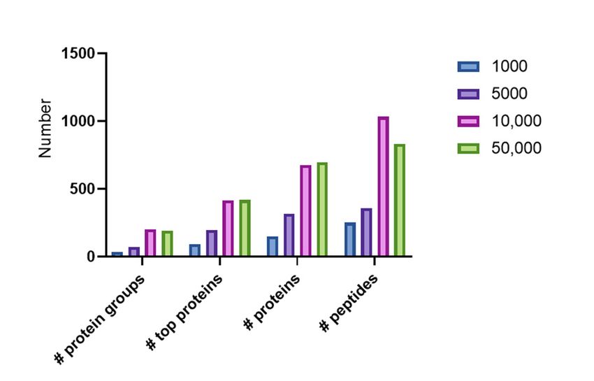
Int. J. Mol. Sci. 2020, 21, x FOR PEER REVIEW 5 of 12
Table 3. Overview of the number (#) of protein identification groups, top proteins, peptides, and
Int. J. Mol. Sci. 2020, 21, 6557 5 of 12
peptide-spectrum matches (PSMs) of five replicates of 1 ng of HeLa protein acquired with the
sensitive method.
Table 3. Overview of the number (#) of protein identification groups, top proteins, peptides,
Name # Protein Groups # Top Proteins # Peptides # PSMs
and peptide-spectrum matches (PSMs) of five replicates of 1 ng of HeLa protein acquired with
Rep 1 20 126 45 128
the sensitive method.
Rep 2 20 106 50 131
Rep 3 # Protein Groups
Name 18 107
# Top Proteins 56
# Peptides 140
# PSMs
Rep
Rep 1 4 2017 126 97 45 44 110
128
Rep
Rep 2 5 2017 106 90 50 40 128
131
Rep 3 18 107 56 140
Rep 4two other minimal
Subsequently, 17 97 MS/MS settings
AGC target 44 are tested110
to see whether changes
Rep 5 17 90 40 128
in the signal intensity threshold can still increase the number of identifications in these low amount
samples. Additionally, we also tested whether an influence of the injection volume of the sample (1
vs.Subsequently, twoisother
10 µL injection) minimal
observed. As AGC targetno
expected, MS/MS settings
influence arevolume
of the tested toofsee whether
sample changes
injection was
in observed.
the signalHowever,
intensity threshold can AGC
lowering the still increase
thresholdthehas
number of identifications
consequences in these
on the number of low amount
identifications
samples.
leadingAdditionally, we alsooftested
to higher numbers PSMswhether
(Figure an
2). influence of the injection volume of the sample (1 vs.
10 µL injection) is observed. As expected, no influence of the volume of sample injection was observed.
However, lowering the AGC threshold has consequences on the number of identifications leading to
higher numbers of PSMs (Figure 2).
Figure 2. The number of protein groups, top proteins, and peptides based on different injection volumes
(1 Figure
or 10 µL)
2. and
Theautomated
number ofgain control
protein (AGC)top
groups, andproteins,
injectionand
timepeptides
(IT) settings.
based on different injection
volumes (1 or 10 µL) and automated gain
2.4. Application of Method to FACS Sorted Cells control (AGC) and injection time (IT) settings.
2.4.With our optimized
Application proteomics/MS
of Method to acquisition protocol, we next analyzed FACS sorted
FACS Sorted Cells
pre-specified cell populations. We chose to isolate CD14+CD15+ cells, a population of scarcely
With our optimized proteomics/MS acquisition protocol, we next analyzed FACS sorted pre-
present abnormal myeloid cells in whole blood. In the sorting process, different amounts of cells were
specified cell populations. We chose to isolate CD14+CD15+ cells, a population of scarcely present
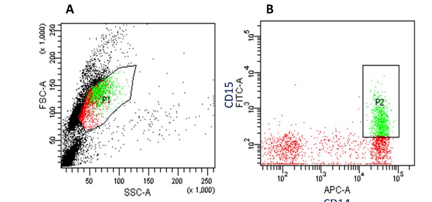
sorted and collected, respectively: 1000, 5000, 10,000, and 50,000 cells. In Figure 3, the gating strategy
abnormal myeloid cells in whole blood. In the sorting process, different amounts of cells were sorted
for the analysis and sorting of double positive cells (P2) and the purity check of the sorted cells (96.5%)
and collected, respectively: 1000, 5000, 10,000, and 50,000 cells. In Figure 3, the gating strategy for the
is depicted.
analysis and sorting of double positive cells (P2) and the purity check of the sorted cells (96.5%) is
Proteomic analysis was performed with the optimized proteomics workflow for FACS sorted
depicted.
samples containing 1000, 5000, 10,000, and 50,000 cells. An overview of the number of protein and
peptide identifications in these samples is represented in Figure 4. In this figure, a distinction is made
between proteins (each protein that is identified in the database and has a different accession number is
counted), top proteins (where proteins with partial sequences are grouped to a top protein), and protein
groups which puts all variants, including proteoforms in a similar group. All protein identifications
are based on the presence of at least one unique peptide.
Int. J. Mol. Sci. 2020, 21, 6557                                                                                             6 of 12
 Int. J. Mol. Sci. 2020, 21, x FOR PEER REVIEW                                                                               6 of 12

         Figure3.3 Gating
       Figure         Gating strategy
                                strategyfor
                                          forthe
                                              theanalysis
                                                    analysisofofCD14+CD15+
                                                                 CD14+CD15+ cellscellsfrom
                                                                                       fromperipheral
                                                                                              peripheralblood
                                                                                                           bloodmononuclear
                                                                                                                  mononuclear
       cells.
         cells.(A)
                (A)Plots
                      Plotsare
                            aregated
                                  gatedononforward
                                            forwardscatter
                                                       scatter(FCS)
                                                                (FCS)and
                                                                      andside
                                                                           sidescatter
                                                                                 scatter(SSC)
                                                                                          (SSC)to todefine
                                                                                                     definethe
                                                                                                            theleukocytes
                                                                                                                leukocytes(P1)
                                                                                                                           (P1)
 Int. J.from
         Mol. cell
         from        debris.
                cell2020,
              Sci.        21, x(B)
                      debris.      Selection
                                 (B)
                                 FOR Selection ofofdouble
                                      PEER REVIEW    doublepositive
                                                             positiveCD14+CD15+
                                                                      CD14+CD15+cell    cellpopulation
                                                                                             population(P2).
                                                                                                           (P2).(C)A
                                                                                                                 (C)Apost-sort
                                                                                                                      post-sort7 of 12
       analysis
         analysison  onP2
                        P2was
                            wasperformed
                                   performedtotodetermine
                                                    determinethethepurity
                                                                    purityofofthe
                                                                               thesorted
                                                                                   sortedcells.
                                                                                            cells.This
                                                                                                   Thissorting
                                                                                                        sortingwas
                                                                                                                 wasconfirmed
                                                                                                                     confirmed
       with
         withaapurity
                 purityofof96.5%.
                               96.5%.

      Proteomic analysis was performed with the optimized proteomics workflow for FACS sorted
 samples containing 1000, 5000, 10,000, and 50,000 cells. An overview of the number of protein and
 peptide identifications in these samples is represented in Figure 4. In this figure, a distinction is made
 between proteins (each protein that is identified in the database and has a different accession number
 is counted), top proteins (where proteins with partial sequences are grouped to a top protein), and
 protein groups which puts all variants, including proteoforms in a similar group. All protein
 identifications are based on the presence of at least one unique peptide.

     Figure 4. Overview of the number of protein groups, top proteins, proteins, and peptides identified
      Figure 4. Overview of the number of protein groups, top proteins, proteins, and peptides identified
     with Peaks X+ in FACS sorted samples on the 1000, 5000, 10,000, and 50,000 cell samples.
      with Peaks X+ in FACS sorted samples on the 1000, 5000, 10,000, and 50,000 cell samples.

      While only three protein groups (representing 148 proteins and 83 top proteins) were detected
 in the sample with 1000 cells, 203 protein groups (representing 677 proteins and 406 top proteins)
 could be detected in a sample with 10,000 cells. Interestingly, a slight decrease in the number of
 identifications with 50,000 cells compared to 10,000 cells is seen. While in 10,000 cells 203 protein
 groups could be identified, only 193 protein groups (compiled from 409 top proteins) were detected
Figure 4. Overview of the number of protein groups, top proteins, proteins, and peptides identified
with Peaks X+ in FACS sorted samples on the 1000, 5000, 10,000, and 50,000 cell samples.
Int. J. Mol. Sci. 2020, 21, 6557 7 of 12
While only three protein groups (representing 148 proteins and 83 top proteins) were detected
in the sample
While onlywith
three1000 cells,groups
protein 203 protein groups 148
(representing (representing
proteins and67783proteins and 406
top proteins) weretop proteins)
detected in
could
the be detected
sample with 1000incells,
a sample with groups
203 protein 10,000 cells. Interestingly,
(representing a slight
677 proteins anddecrease in the number
406 top proteins) could be of
identifications with 50,000 cells compared to 10,000 cells is seen. While in 10,000 cells
detected in a sample with 10,000 cells. Interestingly, a slight decrease in the number of identifications 203 protein
groups
with could
50,000 be compared
cells identified, toonly 193 protein
10,000 groups
cells is seen. (compiled
While from
in 10,000 409203
cells topprotein
proteins) werecould
groups detectedbe
in the 50,000
identified, onlycell sample.
193 proteinThis
groupscan (compiled
be explained fromby409
thetop
factproteins)
that the were
longerdetected
cycle time might
in the be cell
50,000 less
advantageous
sample. This canforbe
higher protein
explained by concentrations.
the fact that theAn overview
longer of allmight
cycle time the top
be protein identifications
less advantageous for
can be found
higher proteininconcentrations.
Supplementary An Table S1.
overview of all the top protein identifications can be found in
Next, we were
Supplementary Tableinterested
S1. to see how many proteins would be commonly identified between the
samples with different amounts
Next, we were interested to see ofhow
cellsmany
(Figure 5). Aswould
proteins the sensitive
be commonlymethod only proved
identified between tothe
be
beneficial
samples fordifferent
with the threeamounts
samplesofwith cells the lowest
(Figure number
5). As of cells,method
the sensitive only a only
comparison
proved to between these
be beneficial
three samples was made.
for the three samples with the lowest number of cells, only a comparison between these three samples
was made.
Figure 5. Qualitative proteomic analysis of different amounts of FACS sorted cells. Venn-diagram
Figure 5. Qualitative
representing an overlapproteomic analysis
in the number of different
of top amounts of
proteins identified FACS sorted
between cells.and
1000, 5000, Venn-diagram
10,000 cells
when either at least one unique peptide per protein is taken into account (left) or when at10,000
representing an overlap in the number of top proteins identified between 1000, 5000, and least cells
two
when either at least one unique peptide per protein is
unique peptides per protein are taken into account (right).taken into account (left) or when at least two
unique peptides per protein are taken into account (right).
Additionally, a two-fold approach was taken. First, we compared the number of top protein
Additionally,
identifications baseda two-fold approach that
on the assumption was attaken.
least First, we compared
one unique peptide the numberper
is required of top protein
protein hit.
identifications
This based us
approach allows on to
the assumption
see how extendedthat the
at least oneprofile
protein unique peptide
can is required
be in this per protein
limited sample hit.
amount.
This approach allows us to see how extended the protein profile can be in this limited sample
With this one peptide per protein rule, 19 top proteins were detected in all three samples, representing amount.
Witha 4%
only thisfraction
one peptide per number
of the total protein ofrule, 19 top identified
top proteins proteins were
across detected in allNot
these samples. three samples,
surprisingly,
these 19 proteins represent high abundant proteins such as different classes of histones (i.e., histone H4,
histone H2B type 1 and Histone 1.2, Histone H2A type 1), vimentin, elongation factor 1-alpha, actin,
and thymosin.
Next, the same analysis was performed but only included proteins that were identified with
minimal two unique peptides were included in the comparison between the different number of sorted
cells to see the potential for future quantitative proteomics work (Figure 6, right panel). Here, only five
proteins (Protein S100-A9, Protein S100-A8, Thymosin beta-4, Histone H4, and dermcidin) representing
only 2% of the dataset were found in each sample. This clearly indicates that extreme caution should
be taken when one would perform quantitative analysis with low sorted cell numbers. However,
even with the two unique peptides per protein rule, 196 top proteins were confidently identified in the
10,000 cell sample.
As only a very limited number of proteins, reflecting only high abundant proteins, were identified
in the 1000 cells and 5000 cells samples, protein profiling of these low cell numbers might not deliver
much insight for downstream proteome analysis. The 10,000 cells sample, on the other hand, has,
with around 200 top proteins, has quite a range of proteins identified., To gain further insights in
the biological function of these proteins, we performed a gene ontology analysis using PANTHER to
classify the identified proteins according to the biological process (Figure 6).identified in the 1000 cells and 5000 cells samples, protein profiling of these low cell numbers might
not deliver much insight for downstream proteome analysis. The 10,000 cells sample, on the other
hand, has, with around 200 top proteins, has quite a range of proteins identified., To gain further
insights in the biological function of these proteins, we performed a gene ontology analysis using
Int. J. Mol. Sci.to
PANTHER 2020, 21, 6557
classify the identified proteins according to the biological process (Figure 6). 8 of 12
Figure 6. Gene ontology analysis of the 414 top proteins identified in the 10,000 cell sample (based on
Figure
the one6.unique
Gene ontology analysis
peptide per of the
protein 414
rule) topvisualized
and proteins identified
accordingin
tothe
the10,000 cell sample
biological process.(based on
the one unique peptide per protein rule) and visualized according to the biological process.
3. Discussion
3. Discussion
The realistic representation of the in vivo proteome of any subclass of cells in a clinical tissue
using Theproteomic techniques is of
realistic representation encumbered by the underlying
the in vivo proteome structure
of any subclass of the
of cells in a heterogeneous
clinical tissue
using proteomic techniques is encumbered by the underlying structure of the of
microenvironment with spatially intermingled distinct cell types. The analysis a single cell
heterogeneous
type can be crucialwith
microenvironment in thespatially
elucidation of cellulardistinct
intermingled functions.
cell To study
types. The cell-specific
analysis ofprotein
a single expression,
cell type
can be crucial in the elucidation of cellular functions. To study cell-specific protein expression,shape,
it is, therefore, critical to employ methods which allow the sorting of cells according to size, it is,
and numerous
therefore, criticalother cell-specific
to employ methodscharacteristics/markers.
which allow the sorting Theofuse of according
cells laser capture microdissection
to size, shape, and
(LCM) to isolate
numerous individual cells
other cell-specific has been implemented
characteristics/markers. in various
The use of laserresearch projects
capture but the fact that
microdissection (LCM)it is
a low-throughput technique and that tissue slices are required for this technology,
to isolate individual cells has been implemented in various research projects but the fact that it is a makes it less-widely
used [9]. Indeed,technique
low-throughput as is also theandcase
thatfor histochemistry,
tissue with LCM
slices are required it is technology,
for this difficult to quantitate the levels of
makes it less-widely
used [9]. Indeed, as is also the case for histochemistry, with LCM it is difficult to quantitate the and
expression because: (1) Tissue sections do not contain intact cells, (2) cells frequently overlap, levels(3)
it is very difficult to discriminate between intermingled positive cells and negative
of expression because: (1) Tissue sections do not contain intact cells, (2) cells frequently overlap, and cells for certain
membrane-bound
(3) it is very difficultproteins [10]. Thebetween
to discriminate use of flow cytometrypositive
intermingled techniques,cellssuch
and as FACS, cells
negative are very helpful
for certain
in these cases. Due to the restricted dimensions of clinical tissues available
membrane-bound proteins [10]. The use of flow cytometry techniques, such as FACS, are very helpful for a wide range of research
questions,
in these cases.FACSDue sorting of arestricted
to the pre-specified type of cells
dimensions results in
of clinical manyavailable
tissues cases onlyforin aa limited
wide rangenumber of
of cells (typically between 1000 and 50,000). In addition to the fact that handling
research questions, FACS sorting of a pre-specified type of cells results in many cases only in a limited a small number of
cells can be detrimental for the overall proteome coverage [11], the incompatibility
number of cells (typically between 1000 and 50,000). In addition to the fact that handling a small of FACS sheath
fluid with proteomics workflows also represents major pitfalls. This makes FACS-based proteomics
not straightforward.
Several studies have already been published where proteomics experiments of a minimal number
of cells were successful. Highes et al. propose a paramagnetic bead technology to eliminate sample
losses during sample preparation of samples limited in quantity [12]. Another machinery is the
proteomic reactor, developed by Ethier et al., where a microfluidic device allows the analysis of
limited amounts of proteins [13]. A miniaturized LC-MS system for the phosphoproteome analysis of
10,000 cells was proposed by Masuda et al. [14]. Sun et al. analyzed femtograms of protein mixtures by
a fast capillary zone electrophoresis-ESI-MS/MS system [15]. The protein content of 100 living cells by
direct cell injection was analyzed by the tool developed by [16]. These minimal cell numbers, however,
are not achieved with the use of cell sorting technologies.
The combination of antibody-based cell purification and proteomics is also previously described.
Di Palma et al. performed a proteomic analysis of 30,000 mice colon stem cells, isolated from
intestine tissue via FACS [17]. The enrichment strategy, however, included the sorting of ‘artificial’
green fluorescent protein (GFP)-expressing cells, rather than membrane-expressing protein targeting.
Wang et al. simulated circulating tumor cells by adding a minimal amount of cultured MCF-7 tumor
cells to whole blood of a healthy volunteer and sorted these MCF-7 out of the blood matrix [18].Int. J. Mol. Sci. 2020, 21, 6557 9 of 12
Although this already resembles more a real-life situation, still no proteomic analysis is performed of a
rare cellular subtype that is isolated via FACS. Additionally, several other studies employ FACS-sorted
cells for proteomic analysis, but they all have large quantities of FACS-sorted cells (ca. 1,000,000 cells),
which made it possible to perform a buffer exchange immediately after FACS sorting and before the
cell pellet is frozen.
To compare protein profiles of rare cell populations, we optimized a workflow that is suitable
for low amounts of cells and that allows us to perform LC-MS after FACS sorting. Our optimized
method clearly demonstrated the benefit for very low amounts of cellular material, with 10,000 cells as
the optimal amount of material. We could demonstrate that the increased cycle time to improve the
MS/MS quality of the acquisition method is, however, only favorable in case ultrasensitive proteomics
is needed due to low protein concentration.
In this preliminary study, we were able to identify 406 top proteins, representing 203 protein
groups from 10,000 CD14+ CD15+ cells in a single LC-MS/MS run. These findings are in line with the
FACS sorted experiment described by Di Palma et al., where an 1D-LC experiment of 5000 GFP-sorted
cells delivered 380 protein identifications [17]. However, when applying the two unique peptides
per protein rule for protein identification, the number of top protein identification drops to 196,
demonstrating that for quantitative proteomics purposes, still only a limited number of proteins
are detected.
Differences in numbers of protein identification between 10,000 and 1000 cells are still almost
5-fold, indicating that even longer cycle times might be more optimal for 1000 cell samples, and that
these very low amounts of cells are still suboptimal for further downstream analysis. However,
our 10,000 cell sorted sample demonstrated great potential in the protein profile context. Therefore,
a gene ontology analysis was performed to generate an overview of the variety of biological processes
the identified proteins are involved in. As expected from immune cells, processes such as response to
stimuli or immune response, as well as processes linked to localization and locomotion are detected,
amongst the more general cellular and metabolic processes.
In conclusion, these results indicate that we are at the next step in fulfilling the technology
requirements towards cell-species-specific proteomics. When proteomics analysis of minimal cell
numbers can be achieved, new insights in cellular heterogeneity in clinical tissues might be untangled.
4. Materials and Methods
4.1. PBMC Isolation and Cell Sorting
Peripheral blood from a healthy volunteer was obtained under consent. The study was conducted
in accordance with the Declaration of Helsinki, and the protocol was approved by the Ethics Committee
of Antwerp University Hospital (No. 12/7/69). Approximately 20 mL of blood was collected in
k2 EDTA vacutainer blood tubes by venous puncture. Samples were processed within two hours after
collection. Peripheral blood mononuclear cells (PBMCs) were isolated by density gradient centrifugation
(Ficoll-Paque TM Plus, GE Healthcare, Chalfont St. Giles, UK) according to the manufacturer’s instructions.
As PBMCs still represent a heterogeneous mixture of immune cells, we further isolated a specific cell type
by fluorescent activated cell sorting (FACS). To reflect the low abundance of a specific type of immune cells
in tumor tissues, CD14+CD15+ cells were sorted. Direct immunofluorescence staining was performed
with the following fluorochrome-labeled mouse anti-human antibodies: Anti-CD14-allophycocyanin
(APC), anti-CD15-fluorescein isothiocyanate (FITC), and anti-CD34-phycoerythrin (PE). For each
sample, at least 50,000 events were recorded using a BD FACSAria II flow cytometer (BD Biosciences,
Franklin Lakes, NJ, USA). The obtained sorted cell pellets, ranging from 1000 to 50,000 cells were
stored at −80 ◦ C until further use.Int. J. Mol. Sci. 2020, 21, 6557 10 of 12
4.2. Sample Preparation of FACS Sorted Cells
The FACS sorted cell pellets were lysed using a RIPA buffer (1×) (Thermo Scientific, Rockford, IL,
USA). Depending on the number of cells, different amounts of RIPA buffer were used: An addition of
10 µL RIPA in 1000 and 5000 cells samples, 20 µL with 10,000 cells, and 100 µL with 50,000 cell pellets.
Additionally, 0.1% of 1 × HALT phosphatase inhibitor (Thermo Scientific) and 1 × HALT protease
inhibitor (Thermo Scientific) were added to each sample. Cell disruption was performed by a 30 s
sonication (Branson Sonifier SLPe ultrasonic homogenizer, Labequip, Markham, ON, Canada) of the
sample on ice followed by a centrifugation of the samples for 15 min at 14,000× g and 4 ◦ C. Afterwards,
the pellet was discarded and four volumes of ice-cold acetone (1:4 volumes acetone) were added to
each supernatant and incubated at −20 ◦ C overnight. The next day, the samples were centrifuged at
14,000× g and 4 ◦ C for 15 min followed by the removal of the acetone. An additional wash with 1 mL
of ice-cold acetone (−80 ◦ C) was performed and after centrifugation (14,000× g, 4 ◦ C, 10 min), acetone
was removed, and the pellet was air-dried for 10 min. Next, the protein pellet was resuspended in
10 µL of a 200 mM TEAB solution.
Next, proteins were reduced by adding 0.5 µL (1000, 5000, and 10,000 cells) or 1 µL (50,000 cells) of
50 mM tris(2-carboxyethyl) phosphine (Thermo Scientific) and incubated for 1 h at 55 ◦ C. Subsequently,
cysteines were alkylated by adding 0.5 µL (1000, 5000, or 10,000 cells) or 1 µL (50,000 cells) 375 mM
iodoacetamide followed by a 30 min incubation in the dark. Again, the sample is precipitated with
acetone by the addition of four volumes of ice-cold acetone per volume of sample and a two-hour
incubation at −20 ◦ C. After centrifugation (14,000× g, 4 ◦ C, 10 min), acetone was removed, and the
pellet was air-dried for 10 min. Next, all protein pellets were resuspended in 10 µL of a 200 mM TEAB
solution and trypsin gold (Promega, Madison, WI, USA) was added to a final concentration of 5 ng/µL
and incubated overnight at 37 ◦ C. Afterwards, samples were stored at −80 ◦ C until further analysis.
4.3. Reversed-Phase Liquid Chromatography and Mass Spectrometry
The peptide mixtures were separated by reversed-phase chromatography on an Easy nLC
1000 (Thermo Scientific) nano-UPLC system using an Acclaim C18 PepMap100 nano-Trap column
(75 µm × 2 cm, 3 µm particle size) connected to an Acclaim C18 Pepmap RSLC analytical column
(50 µm × 15 cm, 2 µm particle size) (Thermo Scientific). Before loading, the sample was dissolved in
10 µL of mobile phase A (0.1% formic acid in 2% acetonitrile. A linear gradient of mobile phase B
(0.1% formic acid in 98% acetonitrile) from 2 %to 35% in 50 min followed by a steep increase to 100%
mobile phase B in 5 min flowed by a 5 min period of 100% B was used at a flow rate of 300 nL/min.
The nano-LC was coupled online with the mass spectrometer using a stainless-steel nano-bore Emitter
(Thermo scientific) coupled to a Nanospray Flex ion source (Thermo Scientific).
The Q Exactive Plus (Thermo Scientific) was used in two different settings: A standard data
dependent analysis (DDA) method and a DDA method tuned for higher sensitivity.
The standard shotgun method was set up in MS/MS mode where a full scan spectrum (350–1850 m/z,
resolution 70,000) was followed by a maximum of twenty HCD tandem mass spectra in the orbitrap,
at a resolution of 17,500. A maximum inject time of 100 ms was set in the full MS, and 80 ms in
MS2. The normalized collision energy used was 27 and the minimal AGC target was set at 1.7 × 10³ .
An isolation window of 1.6 m/z and isolation offset of 0.3 m/z was applied. We assigned a dynamic
exclusion list of 20 s.
In the sensitive method, a full MS spectrum was acquired at a resolution of 70,000 and a mass
range of 350–1850 m/z with a max inject time of 250 ms. Tandem mass spectra (Top 8) were acquired at
a resolution of 35,000, with a maximum inject time of 250 ms, a dynamic exclusion of 10 s, an isolation
window of 1.6 m/z, isolation offset of 0.3 m/z, and a normalized collision of 27. The minimal AGC
target was set at 1 × 10⁴ .Int. J. Mol. Sci. 2020, 21, 6557 11 of 12
4.4. Data Analysis
The PEAKS X+ Studio data analysis software package (Bio informatic Solutions Inc., Waterloo,
ON, Canada) was used to analyze the LC-MS/MS data. The raw data were refined by a built-in
algorithm which allows the association of chimeric spectra. The proteins/peptides were identified
with the following parameters: A precursor mass error tolerance of 10 ppm and fragment mass error
tolerance of 0.05 Da were allowed, the Uniprot_Homo Sapiens database (v05.2017) was used, and the
cRAP database was used as a contaminant database. Trypsin was specified as a digestive enzyme
and up to three missed cleavages were allowed. Carbamidomethylation of cysteine was set as fixed
modification. Both oxidation (M) and phosphorylation (STY) are chosen as variable modifications.
A maximum of three post-translational modifications (PTMs) per sample were permitted. The false
discovery rate (FDR) estimation was made based on decoy-fusion. An FDR ofInt. J. Mol. Sci. 2020, 21, 6557 12 of 12
6. Grutzkau, A.; Radbruch, A. Small but mighty: How the macs-technology based on nanosized
superparamagnetic particles has helped to analyze the immune system within the last 20 years. Cytom. A
2010, 77, 643–647. [CrossRef] [PubMed]
7. Kelstrup, C.D.; Young, C.; Lavallee, R.; Nielsen, M.L.; Olsen, J.V. Optimized fast and sensitive acquisition
methods for shotgun proteomics on a quadrupole orbitrap mass spectrometer. J. Proteome. Res. 2012,
11, 3487–3497. [CrossRef] [PubMed]
8. Sun, B.; Kovatch, J.R.; Badiong, A.; Merbouh, N. Optimization and modeling of quadrupole orbitrap
parameters for sensitive analysis toward single-cell proteomics. J. Proteome Res. 2017, 16, 3711–3721.
[CrossRef] [PubMed]
9. Shapiro, J.P.; Biswas, S.; Merchant, A.S.; Satoskar, A.; Taslim, C.; Lin, S.; Rovin, B.H.; Sen, C.K.; Roy, S.;
Freitas, M.A. A quantitative proteomic workflow for characterization of frozen clinical biopsies: Laser capture
microdissection coupled with label-free mass spectrometry. J. Proteom. 2012, 77, 433–440. [CrossRef] [PubMed]
10. Corver, W.E.; Fleuren, G.J.; Cornelisse, C.J. Software compensation improves the analysis of heterogeneous
tumor samples stained for multiparameter DNA flow cytometry. J. Immunol. Methods 2002, 260, 97–107.
[CrossRef]
11. Wang, F.; Chen, R.; Zhu, J.; Sun, D.; Song, C.; Wu, Y.; Ye, M.; Wang, L.; Zou, H. A fully automated system
with online sample loading, isotope dimethyl labeling and multidimensional separation for high-throughput
quantitative proteome analysis. Anal. Chem. 2010, 82, 3007–3015. [CrossRef] [PubMed]
12. Hughes, C.S.; Foehr, S.; Garfield, D.A.; Furlong, E.E.; Steinmetz, L.M.; Krijgsveld, J. Ultrasensitive proteome
analysis using paramagnetic bead technology. Mol. Syst. Biol. 2014, 10, 757. [CrossRef] [PubMed]
13. Ethier, M.; Hou, W.; Duewel, H.S.; Figeys, D. The proteomic reactor: A microfluidic device for processing
minute amounts of protein prior to mass spectrometry analysis. J. Proteome. Res. 2006, 5, 2754–2759.
[CrossRef] [PubMed]
14. Masuda, T.; Sugiyama, N.; Tomita, M.; Ishihama, Y. Microscale phosphoproteome analysis of 10,000 cells
from human cancer cell lines. Anal. Chem. 2011, 83, 7698–7703. [CrossRef] [PubMed]
15. Sun, L.; Zhu, G.; Zhao, Y.; Yan, X.; Mou, S.; Dovichi, N.J. Ultrasensitive and fast bottom-up analysis of
femtogram amounts of complex proteome digests. Angew. Chem. Int. Ed. Engl. 2013, 52, 13661–13664.
[CrossRef] [PubMed]
16. Chen, Q.; Yan, G.; Gao, M.; Zhang, X. Ultrasensitive proteome profiling for 100 living cells by direct cell
injection, online digestion and nano-lc-ms/ms analysis. Anal. Chem. 2015, 87, 6674–6680. [CrossRef]
[PubMed]
17. Di Palma, S.; Stange, D.; van de Wetering, M.; Clevers, H.; Heck, A.J.; Mohammed, S. Highly sensitive
proteome analysis of facs-sorted adult colon stem cells. J. Proteome. Res. 2011, 10, 3814–3819. [CrossRef]
[PubMed]
18. Wang, N.; Xu, M.; Wang, P.; Li, L. Development of mass spectrometry-based shotgun method for proteome
analysis of 500 to 5000 cancer cells. Anal. Chem. 2010, 82, 2262–2271. [CrossRef] [PubMed]
19. Mi, H.; Muruganujan, A.; Huang, X.; Ebert, D.; Mills, C.; Guo, X.; Thomas, P.D. Protocol update for large-scale
genome and gene function analysis with the panther classification system (v.14.0). Nat. Protoc. 2019,
14, 703–721. [CrossRef] [PubMed]
© 2020 by the authors. Licensee MDPI, Basel, Switzerland. This article is an open access
article distributed under the terms and conditions of the Creative Commons Attribution
(CC BY) license (http://creativecommons.org/licenses/by/4.0/).You can also read