FABADA Fully Adaptive Bayesian Algorithm for Data Analysis
←
→
Page content transcription
If your browser does not render page correctly, please read the page content below
IEEE TRANSACTIONS ON IMAGE PROCESSING - SUBMITTED                                                                                       1

                                                        Fully Adaptive Bayesian Algorithm for Data Analysis
                                                                             FABADA
                                                                                    Pablo M. Sánchez Alarcón, Yago Ascasibar Sequeiros

                                                  Abstract—The aim of this paper is to describe a novel non-           the effects of random noise [1], [2]. Nowadays there is a large
                                               parametric noise reduction technique from the point of view of          number of smoothing algorithms, based on many different
                                               Bayesian inference that may automatically improve the signal-           techniques, see [3] for a review, such as central moving
                                               to-noise ratio of one- and two-dimensional data, such as e.g.
arXiv:2201.05145v1 [astro-ph.IM] 13 Jan 2022

                                               astronomical images and spectra. The algorithm iteratively              average, data grouping/segmentation [4], fitting smooth func-
                                               evaluates possible smoothed versions of the data, the smooth            tions, different types of statistical analysis, partial differen-
                                               models, obtaining an estimation of the underlying signal that is        tial equations, wavelength transformation filters, linear and
                                               statistically compatible with the noisy measurements. Iterations        nonlinear filtering, sparse models and nonlocal self-similarity
                                               stop based on the evidence and the χ2 statistic of the last smooth      models [5] and more recently artificial neural networks, see
                                               model, and we compute the expected value of the signal as a
                                               weighted average of the whole set of smooth models. In this             [6], [7]. Rest of these methods rely on some explicit or
                                               paper, we explain the mathematical formalism and numerical              implicit assumptions about the true (noise-free) signal in order
                                               implementation of the algorithm, and we evaluate its performance        to separate it properly from the random noise. A common
                                               in terms of the peak signal to noise ratio, the structural similarity   assumption is that the signal being retrieved varies gradually
                                               index, and the time payload, using a battery of real astro-             and that the data can be fit by a smooth function, see [8].
                                               nomical observations. Our Fully Adaptive Bayesian Algorithm
                                               for Data Analysis (FABADA) yields results that, without any                Many techniques analyze the probability that the data
                                               parameter tuning, are comparable to standard image processing           correspond to a random Gaussian realization of the model
                                               algorithms whose parameters have been optimized based on the            that attempts to describe the underlying signal plus random
                                               true signal to be recovered, something that is impossible in a          fluctuations of known amplitude [9]. In this work we use
                                               real application. State-of-the-art non-parametric methods, such         Bayesian inference to evaluate and combine different candidate
                                               as BM3D, offer a slightly better performance at high signal-to-
                                               noise ratio, while our algorithm is significantly more accurate         models that iteratively attempt to improve the quality of the
                                               for extremely noisy data (higher than 20 − 40% relative errors, a       fit to the data. This new Bayesian technique incorporates an
                                               situation of particular interest in the field of astronomy). In this    automatic selection criterion based on the statistical properties
                                               range, the standard deviation of the residuals obtained by our          of the residuals, and therefore it yields a fully non-parametric
                                               reconstruction may become more than an order of magnitude               method. Although the motivation of our scheme is the ap-
                                               lower than that of the original measurements. The source code
                                               needed to reproduce all the results presented in this report,           plication in the field of astronomy, our new algorithm, Fully
                                               including the implementation of the method, is publicly available       Adaptive Bayesian Algorithm for Data Analysis FABADA is
                                               at https://github.com/PabloMSanAla/fabada.                              focused in an general way, and it is possible to generate a
                                                 Index Terms—Image denoising, Bayes’ methods, Data analysis,           smooth model for any type of data. Several algorithms have
                                               Astronomy.                                                              been developed over the years for denoising data, and their
                                                                                                                       ability to recover the underlying signal from an experimental
                                                                                                                       data set with its corresponding errors has been evaluated
                                                                      I. I NTRODUCTION                                 and compared according to different standard metrics. Our

                                               T     HE acquisition of any kind of experimental data is
                                                     affected by several sources of statistical error, which
                                               ultimately translate into a random noise component in the
                                                                                                                       method is fully described in Section II, and we use a set of
                                                                                                                       synthetic tests to compare it with other prescriptions in the
                                                                                                                       literature. Details of the comparison procedure are provided
                                               measurements to be recorded. There are different types of               in Section III, and results are discussed in Section IV. Our
                                               noise depending on their physical origin, both related to               main conclusions are succinctly summarized in Section V.
                                               electronic (thermal noise, fluctuations) and mechanical (non-
                                               perfect lenses, antennas, etc.) devices. In astronomy, for ex-
                                                                                                                                                II. FABADA
                                               ample, errors can be produced in the acquisition of the images
                                               due to defects in the optics of the telescopes and in the read-           The goal of our algorithm, FABADA is to estimate an
                                               out process of the detector (typically a CCD) transforming              unknown signal y = y(x) at NX different locations x ∈ X
                                               the light captured by the telescope into an electrical signal.          specified by a 1D or 2D coordinate that belongs to the data
                                               The noise introduced can sometimes be comparable to or                  domain. Its input are NX independent measurements, contam-
                                               even larger than the signal, and different image processing             inated with random Gaussian white noise η(x) ∼ N (0, e(x)),
                                               algorithms may be used to recover the information that is               and the associated errors e = e(x). The noisy observational
                                               buried deep in the data.                                                data, z : X → R, have the form z(x) = y(x) + η(x), and
                                                  Smoothing, where measurements are weighted at nearby                 FABADA returns an estimation ŷ = ŷ(x) of the original signal
                                               spatial or temporal points (using different schemes to assign           y(x) that is statistically compatible with the measurements
                                               weights), is one of the most popular techniques to mitigate             z(x).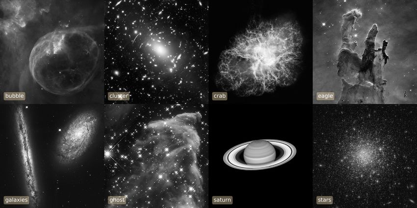
IEEE TRANSACTIONS ON IMAGE PROCESSING - SUBMITTED                                                                                                     2

   For this purpose we apply the Bayes’ theorem in an itera-          our method is to use information from neighboring points to
tively way to generate smooth models of the noisy measure-            update our priors regarding the correct value of m(x). For
ments. Therefore, we must define a suitable likelihood function       every iteration i > 0, the prior probability distribution
to evaluate these models to be tested, and specify a prior                                                       [µ̃i−1 (x)−mi (x)]2
                                                                                                           −
probability distribution for the signal y to initiate the process.                                     e              2·vi−1 (x)

Our likelihood is based on the statistics of a Gaussian process,                      p(mi (x)) = p                                                 (5)
                                                                                                   2π · vi−1 (x)
and we start from an improper, constant prior. Then, we
evaluate different smooth versions of the posterior probabilities     becomes a Gaussian centered on the smoothed expectation (4)
until a certain condition is reached, and we combine all the          of the posterior distribution from the previous iteration, using
smooth models to produce the final estimation ŷ(x), taking           its local variance vi (x) as a measure of our uncertainty.
into account both their Bayesian evidence and the χ2 of the              We stress that we are forsaking the strict Bayesian philos-
residuals.                                                            ophy (the prior distribution should be, as its name indicates,
                                                                      totally independent from the data) on purely practical grounds.
                                                                      Once we accept this premise, one may compute the posterior
A. Iterative models
                                                                      probability distribution
   FABADA, as the name suggests, is a fully automatic algo-
                                                                                                                   [µi (x)−mi (x)]2
rithm that only takes the data set z = z(x) and its associated                                                 −
                                                                                                           e             2vi (x)

errors e = e(x) as input, I = {z, e}, where the domain X may                          P(mi |z, e) =               p                    ,            (6)
                                                                                                                      2πvi (x)
have one or two dimensions. Within the field of astrophysics,
y may be, for example, the spectral energy distribution as a          where
function of wavelength x, or a broadband photometric image                                                 µ̃i−1 (x)   z(x)
                                                                                   µi (x) = vi (x) ·                 + 2                            (7)
of an arbitrary region of the sky. This is indeed the kind of data                                         vi−1 (x)   e (x)
that we will use to illustrate the performance of the algorithm,      and
but the results can be easily generalized to any other type of                             1       1     1
                                                                                               = 2   +         ,                                    (8)
empirical measurement in one or two dimensions affected by                              vi (x)  e (x) vi−1 (x)
Gaussian random errors.
                                                                      as well as the evidence
   Under this assumption, the likelihood function L for a
                                                                                                           [µ̃      (x)−z(x)]2
model m(x) of the underlying signal y is given by                                                     − 2[ei−1
                                                                                                            2 (x)+v
                                                                                                  e                     i−1 (x)]

                                           −
                                             [z(x)−m(x)]2                            Ei (x) = p                                            .        (9)
                                    Y e         2·e(x)2                                           2π[e2 (x) + vi−1 (x)]
        p(z|m, e) = L(z|m, e) =            √                .   (1)
                                    x∈X
                                               2π · e(x)                As long as the model remains relatively p close to the data
                                                                      (within an environment of the order of e2 (x) + vi (x)), the
using the notation described in Table I. Since we do not assume
                                                                      evidence in its favour will be high, but if it departs signifi-
any previous knowledge about the signal, the prior probability
                                                                      cantly, the exponential term will indicate that we have reached
distribution for our initial model m0 will be homogeneous in
                                                                      the maximum smoothing that is statistically compatible with
the range of all possible values, i.e. p(m0 (x)) = 1 for all x,
                                                                      the data.
during the first iteration of the algorithm. According to Bayes’
theorem, the posterior probability distribution
                                                                      B. Stopping criteria
                               p(m) · L(z|m, e)
                P(m|z, e) =                                     (2)    On the one hand, we evaluate the average evidence of model
                                      E
                                                                      mi as
is in this case the straightforward multivariate Gaussian                                        1 X
                                      [z(x)−m0 (x)]2
                                                                                        hEi i =          Ei (x)              (10)
                            Y e−          2·e(x)2
                                                                                                NX
                                                                                                                 x∈X
              P(m0 |z, e) =    √                                (3)
                              x∈X
                                       2π · e(x)                      and we ensure that we iterate until it reaches a maximum;
                                                                      hEi i < hEi−1 i. Since our priors are based on the data them-
centered on the empirical measurements z. The expected value          selves, it is not surprising that the evidence increases rapidly
of m0 (x) is thus µ0 (x) ≡ hm0 (x)i = z(x), its variance              during the first few iterations of the algorithm. However, our
v0 (x) = e2 (x) is determined by the corresponding
                                         R         errors, and        model uncertainties vi (x) decrease monotonically, and the
the Bayesian evidence of the model E = p(m) L(z|m, e) dm              smooth models quickly become less compatible with the data
reduces to unity.                                                     than the first (self-tuned) estimates. Thus, the average evidence
   To create smoothed versions of this first model, we itera-         reaches its maximum at a very early stage, and then it slowly
tively apply a central moving average filter                          declines as the number of iterations increase.
                              P
                               x∈avg µi (x)                              In order to overcome the bias arising from the lack of
                    µ̃i (x) =                               (4)       independence of the priors (i.e. overfitting), we made use of
                                 Navg
                                                                      the chi-square statistics
to the expected values µi (x) of the last iteration. We simply
adopt Navg = 3 in 1D (including the two adjacent measure-                                       X [µi (x) − z(x)]2
                                                                                        χ2i =                                                      (11)
ments) and Navg = 9 (a 3 × 3 square) in 2D. The basis of                                                e2 (x)
                                                                                                x∈X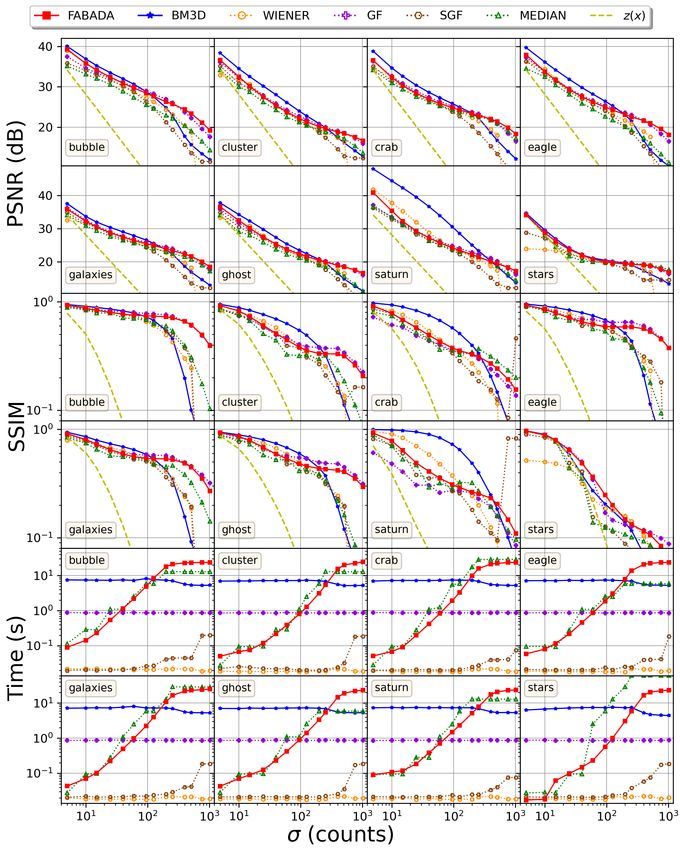
IEEE TRANSACTIONS ON IMAGE PROCESSING - SUBMITTED                                                                                      3

                           Symbol             Definition

 DIMENSIONS                x∈X                Coordinates of the data set (either 1D or 2D coordinates)
                              i               Iteration number {1, 2, , .., Ni }
      INPUTS             I = {z, e}           Set of inputs of the algorithm
                          z = z(x)            Observational measurements
                          e = e(x)            Errors associated to the measurements
     MODELS             mi = mi (x)           Set of all possible models with shape (NX , Ni ).
                         µi = µi (x)          Expectation value of the element x of the model mi
                         vi = vi (x)          Associate variance of the expectation value
                         L(z|mi , e)          Likelihood of the model mi
                           E(mi )             Evidence of the model mi
      PRIORS               p(mi )             Prior probability distribution of the model mi
                             µ̃i              Central moving mean of µi along Navg neighbors
 POSTERIORS              P(mi |z, e)          Posterior probability distribution of the model mi
      OUTPUT              ŷ = ŷ(x)          Estimation of the underlying signal
                                                             TABLE I
                            L IST OF ALL SYMBOLS USED TO DESCRIBE THE FABADA ALGORITHM IN S ECTION II.

and iterate until χ2i > NX − 2 (the absolute maximum of the             give minimal weight to any model that is not extremely close,
associated probability density function). Note that this condi-         χ2 ' NX − 2, which we find tends to yield overly smoothed
tion is achieved when, on average, the model has departed by            models. In order to avoid this problem, we use the actual value
about one sigma from the observational measurements.                    of χ2 to give more weight to the smoother models, but not so
   We always impose both criteria, so that the algorithm stops          much that the models favored by the Bayesian evidence are
on the largest number of iterations. Usually this is set by             almost completely ignored. We thus adopt
the chi-square statistics, although the evidence-based condition
may dominate at very high signal-to-noise ratio.                                                   wi (x) = Ei (x) χ2i ,           (13)

C. Model selection                                                      as our final prescription for i > 0.
   Once the algorithm stops, after Ni iterations, we combine               Of course, this expression is not valid for i = 0, since
all the models mi (x) to generate our final estimation ŷ(x)            χ20 = 0 and the initial evidence is E0 (x) = 1 for every point.
of the real signal y(x) as a weighted sum over the expected             Note that, due to the use of an improper prior, this value is in
values                                                                  general very different from E1 (x). To avoid these problems,
                                                                        we a posteriori set χ20 = χ21 based on the first iteration (i.e.
                          PNi
                                wi (x) µi (x)
                  ŷ(x) = i=0PNi                        (12)            the lowest of all smooth models) and use
                               i=0 wi (x)
                                                                                                                   1
where the adopted weights wi (x) are an important ingredient                                                 e− 2
of our algorithm.                                                                                   E0 (x) = √     ,               (14)
                                                                                                               2πe
   We explored several phenomenological prescriptions in an
attempt to optimize the performance, stability, and reliability         which is merely a reformulation of (9), assuming that our ini-
of the results. On the one hand, our tests show the convenience         tial model based on the measurements should be, on average,
of taking into account the local evidence Ei (x) calculated at          about one sigma away from the true signal. Thus,
each iteration for every location x. This quantity adapts to the                                                       1

local structure of the data, giving more weight to the smoother                                             χ21 e− 2
                                                                                                   w0 (x) = √        .             (15)
models (larger number i of iterations) in areas where the data                                                 2πe
are indeed smooth, while preserving the information when
sharp edges are present.                                                                       III. S YNTHETIC TESTS
   On the other hand, we use the overall χ2i statistic of each
model mi to gauge its compatibility with the measurements z,               We develop a battery of synthetic tests based on real
given the errors e. The probability density function of the χ2          astronomical data to assess the performance of the algorithm.
of a large number of random variables can be approximated as            More precisely, we apply FABADA to a set of astronomical
a narrow Gaussian centered around NX − 2. Since our priors              spectra and images, with different levels of Gaussian random
are biased because they are based on the data themselves, the           noise, and compare the quality of the reconstructed signal (in
maximum evidence occurs at values of χ2 that are typically              terms of the peak signal-to-noise ratio PSNR and the structure
much lower than this value (i.e. they overfit the measure-              similarity index measure SSIM), as well as the execution time,
ments). Using the probability density function directly would           with other methods available in the literature.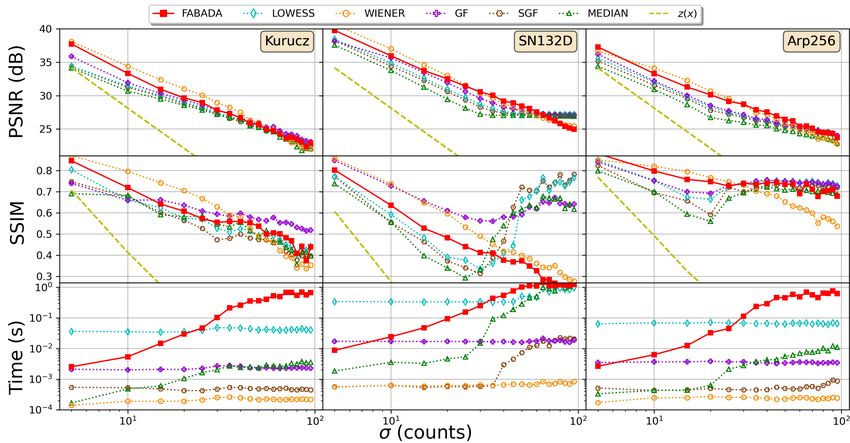
IEEE TRANSACTIONS ON IMAGE PROCESSING - SUBMITTED 4
Method Parameters 1D 2D and independent of the data to be smoothed. Thus,
Median Window size (w) X X w−1
2
w,o
X
SGF Window (w) and order (o) X X ŷSG (x) = Cio (w, o) z(x + i) (16)
GF Radius (R0 ) X X i= 1−w
2
Wiener Low Frequency (k) X X
for w−1 w−1
2 ≤ x ≤ NX − 2 , where the two free parameters of
LOWESS Fraction window (f ) X - the method are the window length w of the data region, i.e.,
BM3D —– - X the number of data points to be fitted, and the order o of the
FABADA —– X X polynomial. Cio are the w ≥ o Savitzky-Golay coefficients, and
w,o
TABLE II
ŷSG (x) is the smoothed result of the filter at position x. We
L IST OF ALL NOISE REDUCTION METHODS USED TO COMPARED WITH vary the window length according to wi+1 = wi +2(1+wi //5)
FABADA ALONG THEIR PARAMETERS AND SPACE IMPLEMENTATIONS , and o ≤ 10 for the order of the polynomial.
ONE OR TWO DIMENSIONS .
3) LOWESS: A popular variant of the Savitzky-Golay
method is the locally weighted scatterplot smoothing
(LOWESS) [2], where the regions to be fitted are not evenly
spaced and the least squares procedure takes into account
A. Other Algorithms
weighted values of the data, according to their distance from
Over the last decades, lots of effort have been placed into the the point to be evaluated. This scheme involves computing
development of several applications that help in the analysis the coefficients of the fitted polynomial each time, producing a
of digital images in different fields. Noise reduction is one of less efficient algorithm. To compare with FABADA we use the
the basic problems in this context, and we attempt to provide implementation explained in [2], which uses a linear fit and can
a fair comparison of our algorithm with other methods that are only be used for one dimensional data. This implementation
representative of the current state of the art. Leaving aside the has only one parameter, which is the fraction f of data points
techniques based on some kind of training, such as e.g. neural used to accomplish the linear regression at each point. For
networks [6], [7], [9], we focus on a more traditional, statistical the optimization we begin with the smallest fraction possible
approach, closer in philosophy to the formalism propose here. (f = 2/NX ) and then it is incremented it by a factor of 1.5
It is important to stress that many of these standard methods until the best recovery is found.
involve a number of free parameters, and we optimize their 4) Gaussian Filter (GF): Another classical technique of
values according to the metrics used to compare. Note that, noise reduction consists in filtering the high frequency com-
of course, such optimization is only possible in a synthetic ponents of the data using a Gaussian filter. The fast Fourier
tests, since the true signal in a real problem is unknown. transform (FFT) is the most computationally efficient way to
Thus, our results represent an upper limit to the performance convert the data z(x) to the frequency domain z̃(w). Once we
of parametric methods. have the spectrum of the image, defined as the amplitude of
the FFT of the data, we can apply a low-pass Gaussian filter
We now briefly describe the main principles and free pa-
to discard the highest modes:
rameters, if any, of all the techniques that we have considered.
2
/2W02
A succinct summary is provided in Table II. GF (z̃(w), W0 ) = e−|z̃(w)| (17)
1) Median filter: One of the classical non-linear digital where |z̃(w)| is the distance from the center (zero frequency
filtering techniques, it is still often used to remove noise from component) in Fourier space, and W0 is the radius of the filter,
an image or signal. The main idea of the median filter is to equivalent to W0 = 2π/R0 in configuration space. This is
run through the data, replacing each point with the median again a one-parameter method, in which we select the radius
of neighboring entries. The number of neighbors used in the R0 of the low-pass Gaussian filter by evaluating in twenty
median is called the ”window”, which slides, entry by entry, logarithmic steps between R0 = 1 and R0 = 630.
over the entire signal. For each data point z(x), the region 5) Wiener Filter: The Wiener filter minimizes the mean
used to compute the median contains, for one dimensional square error taking into account that the measurements are a
data, (w − 1)/2 neighbors on each side, whereas for two random process where the statistical properties (in particular,
dimensions it corresponds to a square of size w centered in the spectrum) of the noise are known. In this work we have
z(x). The optimization procedure consisted on computing the used the implementation in the Scipy Signal Tools library [10],
w
estimation ŷM (x) for different values of w, starting with the [11], where the output of the filter given the signal z(x) is
smallest value of the window length, w0 = 3, and increasing given by
it according to wi+1 = wi + 2(1 + wi //5), where // denotes
the integer division. σ22 mz + 1 − σ22 z σ 2 ≥ σ 2
σz σz z
ŷW (x) = (18)
2) Savitzki-Golay filter (SGF): As first noted by Savitzky m σ2 < σ2
z z
and Golay in [1], a smoothed version of the data may be
obtained by fitting successive sub-sets of adjacent points with where mz and σz2 are local estimates of the mean and variance
a low-degree polynomial using the method of least squares. within a window of size w, and σ 2 = hσz2 (x)i is the the
When the data are equally spaced, the solution of the least average variance across the data. We increment w starting from
squares (i.e., the coefficients of the polynomials) is analytical 3 until the best recovery is found.IEEE TRANSACTIONS ON IMAGE PROCESSING - SUBMITTED 5
Fig. 1. Example spectra used to compare the performance of the different algorithms: a Kurucz stellar atmosphere model (left), supernova remnant N132D
in the Large Magellanic Cloud (center) and interacting galaxy Arp 256 (right).
6) BM3D: Finally, we also include the Block-Matching and with a stellar continuum. The Kurucz and Arp 256 spectra can
3D filtering [4] algorithm, which arguably represents the state be found in the Synthetic Photometry SYNPHOT [15] Python
of the art in the research field of image analysis [9]. A detailed package that simulates photometric data and spectra, observed
account of this method, where image denoising is implemented or otherwise. The aim of using these different spectra is to
as two-step process, can be found in [4]. For the first step, obtain a good representation of the possible features that can
the noisy image is divided into equal-size square blocks. For appear in one-dimensional astrophysical data and see how the
each block, a 3D group is formed with similar regions (block- different algorithms perform in digging up spectral features
matching), and noise is attenuated by hard-thresholding the out of a noisy signal.
coefficients of a 3D transform. The filtered image is used to For astronomical images, we consider eight different targets,
estimate the energy spectrum of the signal, and the process displayed in Figure 2, that are intended to sample the wide
can be repeated a second time using a Wiener filtering instead range of features that may be encountered in the field, includ-
of hard thresholding. The final smoothed result of the image ing planets, stars, diffuse nebulae, and galaxies, either alone
is generated as a weighted average of the denoised blocks in or in potentially blended groups. Saturn is arguably the target
their original positions. This is a non-parametric method, and that is most similar to the ordinary test images (e.g natural
no optimization is necessary. landscapes, human subjects) that are often used in the context
of digital image processing. In addition, our sample includes
two examples of nebulae (Crab and Bubble) dominated by the
B. Data Sample
gaseous component, two with a more significant contribution
All the methods explained in the previous section are of the stellar population (Eagle and Ghost nebulae), and a
applied to a set of test data in one and two dimensions (as- globular cluster full of stars with different brightness. There is
trophysical spectra and monochromatic images, respectively) also an image with a galaxy pair (NGC 4302 & NGC 4298) in
with different levels of Gaussian random noise. which we can see two different orientations of the galaxies, as
An important aspect in the recovery of spectra is the conser- well as a galaxy cluster with a wide variety of morphologies
vation of their features, such as the Balmer break or emission and apparent sizes. All of these images have been taken
and absorption lines, after noise reduction. For this purpose, from the Hubble Space Telescope gallery produced by NASA
we consider three different spectra (represented in Figure 1) and the Space Telescope Science Institute (STScI). All of
that show these characteristics in different degrees. The first them have been compressed to 8-bit values, with a maximal
spectrum (left) is a Kurucz stellar atmosphere model [12] with dynamical range of 0−255 counts and 512×512 pixels size to
an effective temperature Tef f = 11500K, metal abundance lighten up the computational load. For simplicity, we have also
log Z = 0.1 and surface gravity log g = 5.0, typical of an O/B normalized the astronomical spectra to 255 in order to have
type star, with a prominent Balmer break at ∼ 400 nm and the same dynamical range and represent the noise in terms of
several strong absorption lines. The spectrum of a supernova this value for both dimensions.
remnant, plotted on the middle panel, is a composite of 5
different observations [13] from the Faint Object Spectrograph
C. Test Statistics
(FOS) instrument of the Hubble Space Telescope (HST). This
high-resolution spectrum (0.9 Å/pixel) is characterized by We apply different levels of Gaussian random noise η(x)
very prominent emission lines, useful for inferring different with constant variance σ 2 to the real signal y(x):
physical properties of these objects. The last spectrum (right) is z(x) = y(x) + η(x) (19)
taken from the TRDS Brown Atlas [14] which consist on a pair
of interacting galaxies, Arp 256, in the constellation of Cetus, where η(x) = N (0, σ), the element x ∈ X denotes indepen-
and it contains a combination of emission and absorption lines dent measurements (spectrum wavelengths or image pixels),IEEE TRANSACTIONS ON IMAGE PROCESSING - SUBMITTED 6
Fig. 2. Battery of images used for the comparison procedure. From left to right, top to bottom, the objects shown in this figure are the Bubble nebula (NGC
7635), a galaxy cluster (Abell S1063), the Crab nebula (M1), the Eagle nebula (M16), a spiral galaxy pair (NGC 4302 & 4298), the Ghost nebula (IC 63),
Saturn and a globular star cluster (NGC 1466). Labels on the bottom left corner are used to identify each object throughout this work.
and we assume that statistical errors are correctly characterized properties such as luminance, contrast and structure. It is
in the input data. Once z(x) is computed, a softened estimation defined by the expression [16]
ŷ(x) of the real signal y(x) is carried out using the different (2µx µy + C1 ) (2σxy + C2 )
algorithms explained above. SSIM(x, y) = (22)
µ2x + µ2y + C1 σx2 + σy2 + C2
In one dimension, noise levels vary from σ = 5 counts to
σ = 95 counts, out of the 255 maximal value that sets the where x and y denote the two images being compared, µ
dynamical range of our data (i.e. of the order of ≈ 2 − 40% and σ 2 are their mean and variance, and σxy their covariance.
relative errors). We extend the values of σ to even higher The constants C1 and C2 are two variables to stabilize the
values in two-dimensional data, specifically to 1024 counts division when the denominator approaches zero, and they are
(400%) to illustrate the challenging situation (not so seldom usually set to C1 = (0.01 L)2 and C2 = (0.03 L)2 , where
encountered in astronomy) that the signal is actually fainter L is the dynamic range of the images. The SSIM metric can
than the background noise. adopt values from 0 (absolute lack of correlation) to 1 (high
We evaluate the quality of the reconstruction in terms of structural similarity).
the Peak Signal to Noise Ratio (PSNR) and the Structure Another metric that we consider is the CPU time used
Similarity Index Measure (SSIM) of the estimators ŷ(x), to generate the estimation of the real data on a 2.40 GHz
following common practice in the signal processing literature. Intel i9-9980HK CPU along with 16Gb DDR4 2400 MHz
By definition, the PSNR (usually expressed in decibels, dB) RAM memory. Please note that this time corresponds to the
is related to the Mean Square Error (MSE) final execution time for the given noise level in the Python
implementation of the algorithms, once the optimal parameters
1 X 2 have been found, but it does not include the time invested in
MSE(ŷ) = (ŷ(x) − y(x)) (20) the optimization, which is considerably larger.
NX
x∈X
as IV. R ESULTS
2
255 We now assess the ability of our algorithm to recover
PSNR(ŷ) = 10 · log10 , (21)
MSE the underlying signal for the synthetic test cases described
in Section III-B. In order to facilitate the comparison with
where 255 is the dynamical range in our data. In principle, a previous results reported in the literature, we use the Peak
more faithful recovery of the underlying signal should yield Signal-to-Noise Ratio (PSNR) defined in (21), which is just
smaller values of the MSE and higher values of the PSNR. a measure of the Mean Squared Error (MSE), expressed
The Structural Similarity Index Measure (SSIM) is another in decibel (dB), as well as the Structural Similarity Index
typical metric used in image restoration that takes into account Measure (SSIM) defined in (22). All the results shown fromIEEE TRANSACTIONS ON IMAGE PROCESSING - SUBMITTED 7
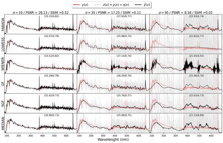
Fig. 3. Results obtained for the Arp 256 spectrum (see figure 1) by all the models explained in section III-A (rows) for three different noise levels (from left
to right columns). The real signal y(x), the noisy input data z(x), and the estimation ŷ(x) are represented as red, gray and black lines, respectively. Numbers
on each panel quote the PSNR and SSIM obtained by each method, to be compared with the noisy data (column headers).
the parametric methods are optimize using the PSNR metric these two recoveries and any of the others. The improvement
(similar results are obtained if SSIM was used instead). with respect to the originally high quality data is necessarily
modest in all cases, of the order of ≈ 3 dB, i.e. an increase
A. Recovery Examples of ∼ 50% in MSE. All algorithms are able to correctly trace
Figures 3 and 4 show two examples of the results obtained the presence of the most prominent emission lines, as well as
by the different algorithms explained in section III-A: the the strong Lyman-α absorption line near the peak at the left
median, Savitzky-Golay filter (SGF), Gaussian Filter (GF), end of the spectrum. Nevertheless, it is important to note that,
Wiener filter, and locally weighted scatterplot smoothing while the Wiener filter provides the best recovery in terms of
(LOWESS) for one-dimensional spectra, and the median, SGF, to the overall noise reduction, FABADA tends to preserve the
GF, Wiener filter and block-matching (BM3D) filters for the true intensity of these features slightly better than any of the
images. Each row of both figures provides the recovered other algorithms.
estimations of the signal ŷ(x) for different noise levels, This trend becomes more significant as the noise increases,
represented in each column. and it is more difficult to discriminate significant spectral
1) Spectra Exmaple: We represent in figure 3 the recoveries features from Gaussian random fluctuations. In the middle
obtained for three random realizations with high, low, and panels, where σ = 35, all models are able to reproduce the
extremely low signal-to-noise ratios (SNR) of the Arp 256 overall shape of the continuum. However, they fail to recover
spectrum (see figure 1). The PSNR achieved by each method even the strongest absorption and emission lines, although
is quoted within the corresponding panel along with the SSIM hints of the brightest emission lines are still present in the
index. Wiener, LOWESS, and GF filters. Only our prescription is able
At high SNR (σ = 10, original PSNR= 28.13 dB, SSIM= to provide a good description of these prominent features with
0.52), all algorithms display not only a similar performance, this level of noise in the input data, albeit weaker absorption
but actually converge to very similar solutions. The highest and emission lines are completely lost. This reflects on the
value of PSNR/SSIM is obtained by the optimized Wiener values of the metrics, where FABADA obtains the highest
filter (33.53 dB / 0.82), a little better than FABADA (33.15 dB values (27.93 dB/0.77); a difference of 10.68 dB, which is
/ 0.82). The difference is lower than the difference between more than an order of magnitude of noise reduction withIEEE TRANSACTIONS ON IMAGE PROCESSING - SUBMITTED 8
Fig. 4. Example of the estimation results for the bubble image (see Figure 2), showing the recoveries for three different values of noise (σ = 15, 95, 255),
i.e. values of PSNR (24.63, 8.59, 0.02) dB and SSIM (0.33, 0.16, 0.002). Rows and columns represent different algorithms and noise levels, respectively,
as indicated by the labels. The last three columns show a close-up of the bubble structure to better gauge the recovery of fine details.
respect to the original measurements. (σ = 95, on the right column), one can see that FABADA
obtains the highest value of PSNR, while GF and LOWESS
If we now turn to the recovery of the most noisy spectrumIEEE TRANSACTIONS ON IMAGE PROCESSING - SUBMITTED 9 obtain higher values of SSIM and close values of PSNR. While values of SSIM in both cases. On the other hand, the GF the results of FABADA and GF are actually similar, all the reaches the highest values of MSE and SSIM, whereas the spectral information in LOWESS is gone. At these high levels median and SGF methods display increasingly lower values of noise, the MSE and the SSIM metrics are rather inadequate than the other methods. Most of them are able to bring up the to assess the quality of the reconstructed emission line spectra, large-scale gradients and structures, but they fail to recover the because they incur in minimal penalty for failing to reproduce smallest filaments (as shown by the zoomed panels) due to the a handful of peaks that are barely statistically significant. The high level of noise. The most significant problem of FABADA criteria implemented in FABADA are more conservative, and is still the salt and pepper noise. The Wiener filter, despite a lot of random fluctuations are kept (hence the slightly lower achieving optimal metrics, returns a composition of smoothed SSIM) together with the most significant remains of the actual and noisy regions that hardly reproduces the true underlying signal. It is somewhat remarkable that FABADA manages to signal. This again give us a hint of the MSE and SSIM metric recover the brightest line even at this noise level, at variance may not be the optimal way to quantify the recovery of this with the other methods, while still obtaining high values of the type of images. On the other hand, it is remarkable how the noise reduction metrics. We stress once again that this does not state-of-the-art BM3D method starts to add some artificial necessarily imply a failure of the methods, but of the MSE as a edges to the recovered image. goodness-of-fit indicator. On the other hand, it does highlight If we push the noise even further, as it is often the case in the robustness of FABADA in this respect, although the results practical astrophysical applications, the signal itself is compa- reported here suggest that perhaps the MSE and SSIM is rable to or even lower than the statistical uncertainties. In our not the optimal metric to gauge the quality of the recovered last test, the noise level is σ = 255, equal to the dynamic range solution or, more likely, that it should be complemented with of the original data. The GF obtains again the highest values another test statistic that quantifies information loss and/or of MSE (26.23 dB, 0.39 dB higher than FABADA’s solution), gives more weight to informative features. almost three orders of magnitude of noise reduction, and a 2) Image Example: Similar trends are observed in the SSIM value of 0.74, equal to FABADA’s. It is noteworthy to results obtained for the 2D data. Figure 4 shows the recovery see that these two solutions are far above the rest, by more of the Bubble nebula image for the whole set of different than ≈ 2.5 dB in PSNR and ≈ 0.3 in SSIM. algorithms, represented in each row, with three different noise Upon visual inspection of the different reconstructions, levels (σ = 15, 95, 255) along the columns. The PSNR and including the zoomed region, one can see that almost every SSIM values obtained for each are also shown in each panel, algorithm, except FABADA and GF, produces some artifacts and a close-up of some structures is provided in the last three in the images either at large or small scales. The GF, for columns to illustrate whether the smoothing methods can re- instance, is very efficient at filtering the high-frequency noise, produce their shape and edges. All models yield fairly similar but, by construction, highlights graininess at the characteristic reconstructions for the high signal-to-noise case (σ = 15). scale of the filter. A similar effect is also evident in the SGF The best reconstruction in terms of the MSE and SSIM is and median filters. The Wiener filter still mixes regions with provided by the state-of-the-art BM3D method, that improves very different levels of smoothing, while BM3D is extremely the PSNR from 24.63 dB to 35.30 dB, more than one order of successful in eliminating the high-frequency ’grain’, albeit the magnitude of noise reduction in terms of the MSE, and from smooth areas of the real image are transformed into more 0.33 to 0.89 for the SSIM index. This is around 20% more than staggered gradients. This feature might be inherent to the the recovery with FABADA (34.22 dB), which is the second block-matching algorithm, whose aim is to classify similar highest value of MSE and slightly higher than, yet similar to, square sections of the image into groups, thus resulting in the optimized Wiener filter (34.02 dB). In terms of the SSIM, patches with similar gradients and/or edges. The fully auto- the Wiener filter actually yields a value that is 2% higher matic method developed in this work, FABADA, seems to than FABADA. The other classical filters (median, SGF, GF) offer a reasonable compromise solution. At high levels of obtain comparable results when their parameters are tuned to noise, it is able to reduce the MSE and increase the SSIM at minimize the MSE, about ≈ 1 dB (∼ 25%) below FABADA’s the cost of significantly blurring the image, but the introduction solution. Regardless of the MSE and SSIM statistics, the of spurious patterns, apart from salt and pepper noise, is not Wiener filter virtually misses some of the filaments in the as severe as in the other methods. shape of the zoomed structure, while the other classical filters recover some of the shapes, although in a blurrier way than FABADA and BM3D. Visually, the latter reproduces the shape B. Entire database results of the zoomed structure better, both in terms of sharpness and We have computed the PSNR, SSIM and CPU time for smoothness. In particular, several edges in FABADA seem to all data samples, noise levels, and methods as a function of σ, be a little bit more blurry compared to BM3D, together with averaged over ten different random realizations. The number of a clearly visible salt and pepper noise component. cases that a specific algorithm has recovered the best solution, Once again, the advantages of our algorithm become more as well as the average difference with respect to the optimal evident as the noise increases. In the middle range, with a noise choice, are quoted in Table III. level of σ = 95, one may see that FABADA’s difference in 1) One dimension - Spectra: In one dimension (Figure 5), MSE with respect to BM3D decrease to 0.6 dB and increases FABADA behaves very similarly to the optimized Wiener to 1.11 dB with respect to the Wiener filter, achieving higher filter, particularly in terms of PSNR (top panel). In general,
IEEE TRANSACTIONS ON IMAGE PROCESSING - SUBMITTED                                                                                                           10

                               1D                                                                     2D
                  PSNR (dB)                  SSIM                                      PSNR (dB)                                    SSIM
 Method                all σ                 all σ           Method           all σ                σ > 95              all σ                   σ > 95
               #max             δ      #max           δ                #max            δ      #max          δ   #max            δ      #max             δ
 FABADA          18            0.511    2            0.137   FABADA      20           1.457    20       0.475      6           0.098       4       0.074
 LOWESS           0            1.072    9            0.069   BM3D        63           1.422    10      2.838      58           0.102       9       0.197
 WIENER           19           0.535    13           0.139   WIENER      0            5.382    0       7.804       2           0.181       2       0.237
 GF              14            0.751    23           0.034   GF          25           1.501    22      0.537      39           0.107       34       0.061
 SGF              6            1.241    10           0.081   SGF         0            4.400    0       5.301       3           0.179       3       0.199
 MEDIAN           0            1.737    0            0.100   MEDIAN      4            3.131    4       2.277       4           0.181       4       0.179
                                                                       TABLE III
  TABLE SHOWING THE NUMBER OF TRIES THAT A SPECIFIC ALGORITHM HAVE RECOVERED THE BEST SOLUTION (#max ) FOR EACH METRIC (PSNR,
        SSIM). A LONG THESE VALUES IT IS SHOWN THE AVERAGE EUCLIDEAN DISTANCE TO THE MAXIMUM VALUE , WHICH WE DEFINED AS
                                                δ =< P SN Rmax (σ) − P SN R(σ) >.

Fig. 5. Peak Signal to Noise Ratios (PSNR), Similarity Structural Indexes (SSIM), and CPU times obtained for all the one dimensional spectra samples
and noise ranges considered in the comparison procedure. In the top set of figures is shown the PSNR in decibels (dB), in the middle is represented the
SSIM, and in the bottom one the CPU time in seconds (s). Each figure of both groups is labeled with the reference name given at the top of the column.
The dashed yellow line represents the PSNR and SSIM of the noisy data. Solid lines with filled symbols refers to the non-parametric methods. In 1D data
the only automatic method is the one presented in this work, FABADA, an it is represented with a red solid square (). Dotted lines with unfilled symbols
                                                                                                                                           ◦
refers to the optimize methods. The LOWESS algorithm is represented with the blue diamond (♦), the Wiener filter with the orange circle ( ), GF with the
purple cross ( ), SGF with the brown hexagon (7), and the median filter with the green triangle (4).

the best results regarding this metric are achieved with the                   of the standard methods typically used in astronomy. The
latter method; 19 out of the 57 (33%) test cases, followed                     average difference with respect to the highest PSNR achieved
by FABADA, who obtained the best PSNR for 18 (32%)                             by any algorithm is only 0.511 dB. This supports the idea
estimations, being especially successful in the low signal-                    that FABADA automatically achieves the limit of the standard
to-noise regime. Then, the optimized GF obtained the best                      methods, when their parameters are tuned to the (unknown)
reconstruction in 14 (25%) cases, and the remaining 6 (10%)                    optimal values.
correspond to the optimized SGF. Neither LOWESS nor
                                                                                 In terms of the SSIM metric (middle panels), our algorithm
the median filter obtained in any case the best values for
                                                                               obtains slightly worse results, being the best option only in
PSNR. Just taking into account these results, one can see
                                                                               2 (4%) test cases, with an average distance with respect to
how FABADA preforms as well as the best possible solutions
                                                                               the highest SSIM of 0.137. The optimized GF filter obtained
IEEE TRANSACTIONS ON IMAGE PROCESSING - SUBMITTED 11
Fig. 6. Peak Signal to Noise Ratios (PSNR), Similarity Structural Indexes (SSIM), and CPU times obtained for all the two dimensional images samples and
noise ranges considered in the comparison procedure. In the top set of figures is shown the PSNR in decibels (dB), in the middle is represented the SSIM,
and in the bottom one the CPU time in seconds (s). Each panel is labeled with the reference image name given. The dashed yellow line represents the PSNR
and SSIM of the noisy data. Solid lines with filled symbols refers to the non-parametric methods. In 2D data there are two automatic methods, FABADA,
which it is represented with a red solid square () and the block matching 3D filtering BM3D, with blue stars (H). Dotted lines with unfilled symbols refers
◦
to the optimize methods. The Wiener filter is represented with the orange circle ( ), GF with the purple cross ( ), SGF with the brown hexagon (7), and
the median filter with the green triangle (4).IEEE TRANSACTIONS ON IMAGE PROCESSING - SUBMITTED 12
23 (40%) of the highest values and an average difference of metric FABADA only achieves the best recovery in 6 (5%)
0.034. This result is due in part to the SN 132D spectra, where cases, 4 (7%) at high noise levels, it is only 0.1 apart, on
most of the information is concentrated in the emission lines. average, from the best solution and 0.07 at the high noise
At high values of the noise level, almost all standard methods regime. The optimized GF produces better estimations than
converge towards a horizontal line, where all the information FABADA in 39 (35%) cases, 34 (60%) in the low SNR regime.
is lost (see e.g. LOWESS in Figure 3). However, the SSIM Despite this difference, GF is still 0.1 below the best solution
(and, to some extent, PSNR) do not strongly penalize the mis- (0.06 at low SNR), again very close to the results obtained by
fitting of the emission lines when their statistical significance our algorithm.
becomes low, which hints the limitations of these metrics to This change on the trend of the best solution is at the
quantify the recovery of relevant information. Discarding the cost of CPU time. While FABADA seems to converge to
SN132D spectra, FABADA is seldom the optimal choice, but its solution in an efficient way in the high SNR regime
the average distance decreases to 0.048 in terms of SSIM, (always below the second), for high noise levels (low SNR)
compared to 0.022 for the GF and 0.056 − 0.085 for the other the time rises up to 30 s, as shown in the bottom panels.
algorithms. Once again, for the optimized models we only take into
As regards to the CPU time, it is easy to see that FABADA account the execution time with the fine-tuned parameters
has a strong dependence on the level of noise, at variance already known. The results are similar to the one-dimensional
with most classical methods, due to the increasing number of case, but the time scale increases with the dimensionality of
iterations required to fulfill our χ2 stopping condition. This the problem. The optimized Wiener filter is still the fastest
behavior is also seen in the median, due to a similar increase algorithm, obtaining an average time of 0.02 seconds, while
of the optimal window size, whether other methods are less median filter seems to be the slowest, with 9.34 seconds.
sensitive to the noise level. FABADA is, in general, signifi- FABADA also features a high execution time (8.08 seconds
cantly slower than the other algorthims (except LOWESS, at on average), whereas BM3D, GF, and SGF yield 6.7, 0.87,
high signal-to-noise ratios), although it must be borne in mind and 0.05 seconds, respectively. However, the performance of
that we have not taken into account the time consumed by FABADA and the median filter vary significantly as a function
the optimization process of the standard algorithms, only the of SNR. Combining these results with the above metrics for
execution time once the optimal parameters have been found. the quality of the reconstruction, we argue that our method
2) Two dimensions - Images: For the two-dimensional provides a competitive alternative both at high SNR, where it
images (figure 6) BM3D reaches the highest PSNR for 63 achieves slightly less reliable results than the state-of-the-art
out of our 112 (56%) test cases with different target and algorithm BM3D at a fraction of the computational cost, as
noise levels, followed by the optimized GF with 25 (22%), well as in the low SNR regime, where it provides a more
FABADA with 20 (18%), and 4 (4%) that correspond to the faithful reconstruction after a significantly larger execution
optimized median filter. Neither SGF nor Wiener filter ever time.
obtained the highest values. Nevertheless, BM3D is on average
1.42 dB below the optimal choice, comparable to the 1.46 dB V. C ONCLUSIONS
of FABADA and 1.50 dB of GF, due to the significantly In this work we present the theory and implementation of a
different trends observed at different noise levels. novel automatic algorithm for noise reduction: the Fully Adap-
In general, BM3D stands over the other methods, including tive Bayesian Algorithm for Data Analysis (FABADA). Our
FABADA, at high SNR (σ . 95 dB), in particular for the method iteratively evaluates progressively smoother models of
Saturn image. Its collaborative filter is particularly well suited the underlying signal, and then combines them according to
for periodic data, or images with repetitive patterns, which their Bayesian evidence and χ2 statistic. The source code is
are virtually absent in other test cases. The stars image would publicly available at https://github.com/PabloMSanAla/fabada.
be a paradigmatic example, and the difference in this test is We compare FABADA with other methods that are repre-
insignificant. sentative of the current state of the art in image analysis and
On the other hand, FABADA and GF predominate in the digital signal processing. For this comparison we used the most
low-SNR regime (σ & 95 dB), where BM3D only achieves the typical metrics, the Peak Signal to Noise Ratio (PSNR), which
best reconstruction in 10 out of the 56 (18%) test cases. The is a measure of the Mean Square Error (MSE), the Structural
remaining 46 are achieved by GF with 22 (39%), FABADA Similarity Index (SSIM) and the CPU time. One important
with 20 (36%), and the median filter with 4 (7%). Furthermore, advantage of our method, shared by BM3D, over classical
BM3D is on average 2.84 dB below the highest value, while algorithms is the absence of free parameters to be tuned by
FABADA and GF are only 0.48 and 0.54 dB lower, respec- the user. Our results suggest that FABADA and BM3D achieve
tively. Essentially, FABADA and the optimized GF achieve values of PSNR or SSIM comparable to or better than the best
remarkably similar results, and they preform better than BM3D possible solution attainable by the classical methods.
at low signal-to-noise ratios. Beyond the precise values of the global quantitative metrics,
This behavior is also seen in the middle panels, where the both FABADA and BM3D are quite successful in adapting
SSIM is represented. From the 58 (52%) of the highest values to the structures present in the input data. Perhaps the most
achieved by BM3D, only 9 (20%) are above σ > 95 counts, significant difference between them is that FABADA’s priors
and the difference with respect to the highest value of SSIM assume that the signal is smooth, whereas BM3D uses block-
increases with noise level from 0.1 to 0.2. Although in this matching to look for repetitive patterns. This might be relevantIEEE TRANSACTIONS ON IMAGE PROCESSING - SUBMITTED 13
when one must recover the height and shape of the spectral [15] P. L. Lim, R. I. Diaz, and V. Laidler, “Pysynphot user’s guide
features in 1D or the gradients and boundaries in 2D. We (baltimore, md: Stsci),” 2015. [Online]. Available: http://synphot.
readthedocs.io/en/latest/
argue that FABADA appears to offer a trade-off between [16] Z. Wang, A. Bovik, H. Sheikh, and E. Simoncelli, “Image quality assess-
noise reduction, increasing the metric values significantly, in ment: from error visibility to structural similarity,” IEEE Transactions
a way that is statistically compatible with the data, keeping on Image Processing, vol. 13, no. 4, pp. 600–612, 2004.
significant features without introducing considerable artifacts.
Regarding execution time, non-parametric methods are more VI. ACKNOWLEDGMENTS
expensive than the classical alternatives once the optimal Pablo M. Sánchez-Alarcón acknowledges support from the
values of their parameters are known, something that is of State Research Agency (AEI-MCINN) of the Spanish Ministry
course impossible in practice. FABADA is faster than BM3D of Science and Innovation under the grant ”The structure and
at high SNR, although it usually yields a poorer reconstruction, evolution of galaxies and their central regions” with reference
and the trend reverses for low SNR. PID2019-105602GB-I00/10.13039/501100011033, and from
IAC project P/300724, financed by the Ministry of Science
R EFERENCES and Innovation, through the State Budget and by the Canary
[1] A. Savitzky and M. J. E. Golay, “Smoothing and differentiation of Islands Department of Economy, Knowledge and Employ-
data by simplified least squares procedures.” Analytical Chemistry, ment, through the Regional Budget of the Autonomous Com-
vol. 36, no. 8, pp. 1627–1639, 1964. [Online]. Available: https:
//doi.org/10.1021/ac60214a047
munity. Yago Ascasibar acknowledges financial support from
[2] W. S. Cleveland, “Robust locally weighted regression and smoothing grant ”Starbursts throughout the evolution of the Universe”
scatterplots,” Journal of the American Statistical Association, vol. 74, (PID2019-107408GB-C42) from the AEI-MICINN, Spain.
no. 368, pp. 829–836, 1979. [Online]. Available: https://www.
tandfonline.com/doi/abs/10.1080/01621459.1979.10481038
[3] B. Goyal, A. Dogra, S. Agrawal, B. Sohi, and A. Sharma, “Image
denoising review: From classical to state-of-the-art approaches,”
Information Fusion, vol. 55, pp. 220–244, 2020. [Online]. Available:
https://www.sciencedirect.com/science/article/pii/S1566253519301861
[4] K. Dabov, A. Foi, V. Katkovnik, and K. Egiazarian, “Image denoising by
sparse 3-d transform-domain collaborative filtering,” IEEE Transactions
on Image Processing, vol. 16, no. 8, pp. 2080–2095, 2007.
[5] S. Gu, L. Zhang, W. Zuo, and X. Feng, “Weighted nuclear norm
minimization with application to image denoising,” in 2014 IEEE Pablo Manuel Sánchez Alarcón was born in
Conference on Computer Vision and Pattern Recognition, 2014, pp. Madrid, Spain, in 1996. He received the B.S. de-
2862–2869. gree in physics from the Universidad Autónoma de
[6] A. E. Ilesanmi and T. O. Ilesanmi, “Methods for image denoising using Madrid, Spain in 2019, the M.S. degree in theoretical
convolutional neural network: a review,” Complex & Intelligent Systems, physics from Universidad Autónoma de Madrid and
2021. [Online]. Available: https://doi.org/10.1007/s40747-021-00428-4 the Instituto de Fı́sica Teórica, Madrid, Spain in
[7] K. Zhang, W. Zuo, Y. Chen, D. Meng, and L. Zhang, “Beyond a gaussian 2020. He is currently pursuing the Ph.D. degree in
denoiser: Residual learning of deep cnn for image denoising,” IEEE astronomy, specializing in galaxy evolution, with the
Transactions on Image Processing, vol. 26, no. 7, pp. 3142–3155, 2017. Universidad de La Laguna, Tenerife, Spain. He is
[8] V. Katkovnik, V. Katkovnik, K. Egiazarian, and J. Astola, Local also a researcher at the Instituto de Astrofı́sica de
Approximation Techniques in Signal and Image Processing, ser. Canarias.
SPIE Press monograph. SPIE Press, 2006. [Online]. Available:
https://books.google.to/books?id=YChTAAAAMAAJ
[9] M. El Helou and S. Susstrunk, “Blind universal bayesian image
denoising with gaussian noise level learning,” IEEE Transactions on
Image Processing, vol. 29, p. 4885–4897, 2020. [Online]. Available:
http://dx.doi.org/10.1109/TIP.2020.2976814
[10] P. Virtanen, R. Gommers, T. E. Oliphant, M. Haberland, T. Reddy,
D. Cournapeau, E. Burovski, P. Peterson, W. Weckesser, J. Bright, S. J.
van der Walt, M. Brett, J. Wilson, K. J. Millman, N. Mayorov, A. R. J.
Nelson, E. Jones, R. Kern, E. Larson, C. J. Carey, İ. Polat, Y. Feng, E. W.
Moore, J. VanderPlas, D. Laxalde, J. Perktold, R. Cimrman, I. Henrik- Yago Ascasibar Sequeiros was born in Madrid,
sen, E. A. Quintero, C. R. Harris, A. M. Archibald, A. H. Ribeiro, Spain, in 1975. He received the Ph.D. degree in
F. Pedregosa, P. van Mulbregt, and SciPy 1.0 Contributors, “SciPy 1.0: Astrophysics and Cosmology from the Universidad
Fundamental Algorithms for Scientific Computing in Python,” Nature Autónoma de Madrid, Madrid, Spain, in 2003.
Methods, vol. 17, pp. 261–272, 2020. He held postdoctoral research positions at the
[11] J. S. Lim, Two-dimensional signal and image processing. Englewood University of Oxford, UK, in 2003, the Harvard-
Cliffs, N.J. ; Prentice Hall, 1990. Smithsonian Center for Astrophysics, USA, in 2004,
[12] F. Castelli and R. L. Kurucz, “New Grids of ATLAS9 Model Atmo- the Leibnitz Institut für Astrophysik Potsdam, Ger-
spheres,” in Modelling of Stellar Atmospheres, N. Piskunov, W. W. many, in 2005, and the Universidad Autónoma de
Weiss, and D. F. Gray, Eds., vol. 210, Jan. 2003, p. A20. Madrid, Spain, in 2008. He is currently Associate
[13] W. P. Blair, J. A. Morse, J. C. Raymond, R. P. Kirshner, J. P. Hughes, Professor at that institution, since 2019. His main
M. A. Dopita, R. S. Sutherland, K. S. Long, and P. F. Winkler, “Hubble research interests are galaxy formation and evolution, dark matter, statistics
Space Telescope Observations of Oxygen-rich Supernova Remnants in and data analysis.
the Magellanic Clouds. II. Elemental Abundances in N132D and 1E Dr. Ascasibar is member of the Spanish Astronomical Society, European
0102.2-7219,” Astrophysical Journal, vol. 537, no. 2, pp. 667–689, Jul. Astronomical Society, and International Astronomical Union.
2000.
[14] M. J. I. Brown, J. Moustakas, J. D. T. Smith, E. da Cunha, T. H. Jarrett,
M. Imanishi, L. Armus, B. R. Brandl, and J. E. G. Peek, “An Atlas of
Galaxy Spectral Energy Distributions from the Ultraviolet to the Mid-
infrared,” Astrophysical Journal, Supplement, vol. 212, no. 2, p. 18, Jun.
2014.You can also read