European cephalopods distribution under climate change scenarios
←
→
Page content transcription
If your browser does not render page correctly, please read the page content below
www.nature.com/scientificreports
OPEN European cephalopods distribution
under climate‑change scenarios
Alexandre Schickele*, Patrice Francour & Virginie Raybaud
In a context of increasing anthropogenic pressure, projecting species potential distributional shifts
is of major importance for the sustainable exploitation of marine species. Despite their major
economical (i.e. important fisheries) and ecological (i.e. central position in food-webs) importance,
cephalopods literature rarely addresses an explicit understanding of their current distribution and the
potential effect that climate change may induce in the following decades. In this study, we focus on
three largely harvested and common cephalopod species in Europe: Octopus vulgaris, Sepia officinalis
and Loligo vulgaris. Using a recently improved species ensemble modelling framework coupled with
five atmosphere–ocean general circulation models, we modelled their contemporary and potential
future distributional range over the twenty-first century. Independently of global warming scenarios,
we observed a decreasing in the suitability of environmental conditions in the Mediterranean Sea and
the Bay of Biscay. Conversely, we projected a rapidly increasing environmental suitability in the North,
Norwegian and Baltic Seas for all species. This study is a first broad scale assessment and identification
of the geographical areas, fisheries and ecosystems impacted by climate-induced changes in
cephalopods distributional range.
Cephalopods represent a major and increasingly targeted group by fisheries worldwide with annual landings
ranging from 2 million tons in 1980 to 4 million tons in 2010 (c.a. 2–4% of global annual landings), respectively
generating 3 to 8 billion US$ per year (c.a. 2–5% of global landing value)1. They are intermediate trophic level
and opportunistic species that occupy a central role in the food webs of temperate e cosystems2–4. They feed
mainly on benthic and demersal communities (e.g. fish, crustacean, Mollusca) and are mostly predated by marine
mammals (e.g. seals, cetaceans) and piscivorous fishes (e.g. Sparidae, Serranidae)3. Most cephalopods are short
lifespan species (c.a. 2–4 years) characterised by a rapid growth (i.e. maturity after one winter) and an important
sensitivity to environmental conditions5–7. Environmental stress related to temperature (e.g. heatwaves) or salinity
(e.g. important river discharge) may therefore affect the physiology (e.g. larval survival, growth, reproduction)
of these small bodied and largely dispersing species (i.e. external fecundation, high number of gametes)5,6,8,9. By
affecting these critical lifestages, environmental conditions are also defining the recruitment, abundance and dis-
tribution of cephalopod species5, which may influence their sustainable exploitation and economic importance10.
Since the mid-nineteenth-century, Earth has faced global and unprecedented anthropogenic changes, lead-
ing to an average temperature increase of 0.93 °C11. Temperature is currently increasing at a rate of + 0.2 °C per
decade12, leading to a + 1.5 to + 4.5 °C average temperature increase by the end of the century, depending on global
political, societal and demographical p athways13,14. Global climate change is therefore directly altering the living
15–17
environment of marine species , especially temperature (i.e. yearly average and extreme climatic events) that
is of major importance in the lifecycle of cephalopods (e.g. size and number of eggs, growth rate)5,10,18. In this
context, a global proliferation of cephalopods has been reported in recent y ears19, including locally observed
distributional range shifts and an important climate-induced variability (e.g. spawning season, recruitment) in
temperate seas (e.g. in the North and Yellow seas)20–22. According to these observed distributional and behav-
ioural changes, recent predictions highlighted the potential capacity of cephalopods to extent their distribution
towards the pole, suggesting a future range expansion of these species23–25. In addition, recent studies highlighted
the major economic importance of fisheries for several European c ountries26,27. Medium to long-term distribution
shift of cephalopods—that represent important capture in E urope1,28—may induce major costs and economic
consequences related to an adaptation of their future exploitation s trategies29–31. Anticipating these climate-
induced changes is therefore necessary to avoid abrupt fisheries adaptations at higher costs29. In a context of
severe, climate-induced warming in European seas (up to + 0.35 °C per decade)32,33, a sustainable resource man-
agement perspective34 and the sensitivity of cephalopods to environmental variations10,35, it is therefore of major
importance to project robust scenarios of cephalopod responses to changing environmental conditions in Europe.
These interactions between environmental conditions and species are formalised in the concept of ecologi-
cal niche (sensu Hutchinson)36,37, that is defined as the n-dimensional ensemble of environmental conditions
Université Côte d’Azur, CNRS, UMR 7035 ECOSEAS, Nice, France. *email: alexandre.schickele@univ‑cotedazur.fr
Scientific Reports | (2021) 11:3930 | https://doi.org/10.1038/s41598-021-83457-w 1
Vol.:(0123456789)
www.nature.com/scientificreports/
necessary for a species to live and reproduce. Based on this concept, Species Distribution Models define the
potential distribution of a species according to the same n-dimensional ensemble of environmental conditions in
which the species is observed38,39. Conversely to other modelling approaches (e.g. habitat or ecosystem models),
SDMs are based on occurrence data, encompassing the entire distributional range of a s pecies38. By considering
the entire range of suitable environmental conditions, SDMs are able to estimate the global distributional range
of a species under past, present and future climate conditions39. Ensemble models, that are SDMs constructed
from several statistical algorithms using the same environmental factors, estimate an average species response to
environmental conditions and its related uncertainty, avoiding a-priori assumptions on its shape40–42. Coupled
with several climate models, these multi-algorithm procedures are known to produce a robust assessment of
both contemporary and future distribution as well as the uncertainty associated to niche estimation and climate
projections40–43.
In this study, we projected the contemporary and future potential distributions at the European scale, based
on the outputs of an ensemble model for three cephalopod species common to our study a rea3,7: the common
octopus (Octopus vulgaris; Cuvier, 1797), the common cuttlefish (Sepia officinalis; Linnaeus, 1758) and the com-
mon squid (Loligo vulgaris; Lamarck, 1798). The three considered species are the most representative in terms
of official landings1,28. Moreover, they are broadly distributed in the European seas, overlapping with a large
diversity of environmental conditions. For the three cephalopod species, we projected (i) their contemporary
(1990–2017) distribution and (ii) a range of potential future distributional response to climate change over the
twenty-first century, based on occurrence records and a recently developed ensemble modelling p rocedure44,45.
Our framework integrates a multi-SDM approach (i.e. including the uncertainty between algorithms)40 coupled
with three greenhouse gases emission scenarios (i.e. Representative Concentration Pathways, RCP)13,14 and five
atmosphere–ocean General Circulation Models (GCMs) from the 5th phase of the Coupled Model Intercom-
parison Project, resulting in robust future cephalopod distribution p rojections43. These projections are needed
for medium- to long-term conservation strategies and further operational studies, by identifying geographical
areas where cephalopods may be subject to strong environmental impacts, at large spatial scale.
Materials and methods
Data collection. Cephalopod occurrence records. To avoid a truncated niche estimation and in line with
SDM best p ractices46,47, it is necessary to consider the entire observed distributional range in SDM, indepen-
dently of the study area, to avoid biases in future projections such as an overestimation of potential distributional
range regression46,47. We acknowledge that the plasticity of cephalopod may induce local adaptations to environ-
mental conditions10,19, of interest for regional and integrated studies. However, such adaptations are of negligible
spatial range in our global distributional range estimation48. Therefore, we collected occurrence records for all
studied species, at the global scale, from three available public databases encompassing the up-to-date known
distribution of the three species. The database considered were: the Ocean Biogeographic Information System
(OBIS, http://www.iobis.org/), the Global Biodiversity Information Facility (GBIF, https://www.gbif.org/) and
SeaLifeBase (https://www.sealifebase.org/). To create the most up-to-date observation datasets, we completed
the dataset with observations retrieved from peer-reviewed articles (see Supplementary Appendix 1). We then
performed a data cleaning procedure on each cephalopod dataset to (i) remove unreliable occurrences (e.g.
preserved specimen or taxonomic confusion)49, (ii) discard duplicated records and (iii) ensure their temporal
and locational reliability (e.g. data on land, longitudinal and/or latitudinal inversion). The resulting up-to-date
observation datasets included: 3380 (41 literature-based) occurrences for the common octopus, 4671 (including
17 literature-based) occurrences for the common cuttlefish and 1676 (90 literature-based) occurrences for the
common squid. Conversely to quantitative data (e.g. a number of individuals, biomass or abundance) that highly
depends on the sampling protocol, SDMs only requires georeferenced observations (i.e. occurrence points) to
estimate the environmental conditions in which a species is observed38. Such qualitative data are produced by
various sources, independently of the sampling protocol (e.g. gear, mesh size), allowing scientific survey data to
be included in our datasets (e.g. MEDITS, ICES trawling surveys) as well as diving observations and georefer-
enced fisheries catch. Finally, because the studied cephalopod species are rarely observed below 300 m depth3,7, a
precautionary bathymetry threshold (− 1000 m; due to important bathymetrical variation in the Mediterranean
where the continental shelf is reduced) was applied to remove inconsistent occurrences, at the risk of removing
some deep and uncommon observations. For the three considered species, occurrence data were aggregated on
a 0.1° × 0.1° resolution spatial grid, corresponding to the resolution of environmental factors.
Environmental data. We then collected environmental factors (Table 1) to model the ecological niche (sensu
Hutchinson)36,37 of each cephalopod species. Environmental factors values were first calculated on a yearly basis
and then averaged on the 1990–2017 contemporary period. Among temperature related factors, the Sea Bottom
Temperature (SBT) range was calculated as the difference between the SBT of the warmest month and the SBT
of the coldest month within a year while the SBTvar was calculated as the inter-month SBT variance within a
year. To project the evolution of future environmental factors for a range of radiative forcing13,14, GCMs consider
a large variety of 3-dimensional environmental factors such as ocean circulation, water temperature, salinity,
primary production, carbon cycle dynamics, atmospheric temperature and aerosol concentrations e.g. Refs.50,51.
Without being exhaustive, GCMs projections may diverge for parametrisation reasons such as a spatial resolu-
tion ranging between 0.1° and 0.5°52 or their ability to model carbon or water cycle feedbacks (e.g. influencing ice
cover)33,53,54. Because of their complexity and the absence of a ‘better performing’ GCM, the choice of a unique
algorithm may greatly influence our future distributional range projections43,55. Therefore, following an ensem-
ble modelling p rinciple41 that accounts for uncertainty relative to future environmental factor p rojections40,43,
we considered five commonly used GCMs retrieved from the 5th phase of the Coupled Model Intercompari-
Scientific Reports | (2021) 11:3930 | https://doi.org/10.1038/s41598-021-83457-w 2
Vol:.(1234567890)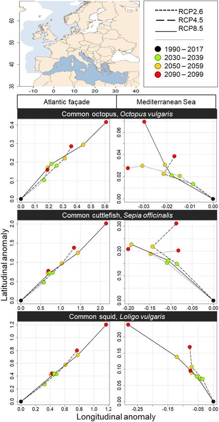
www.nature.com/scientificreports/
Name Description Contemporary (1990–2017) Future (2006–2099)
SSSa Sea surface salinity (‰) Levitus’ climatology56 completed with ICES data (http://www.ices.dk/)
SBTb Mean annual sea bottom temperature (°C)
IPSL50,52, MPI58,59, CNRM51, HadGEM60 and G
ISS61
SBTrangeb Mean annual sea bottom temperature range (°C) CORA: Coriolis Ocean database for ReAnalysis57
models
SBTvarb Mean monthly sea bottom temperature variance (°C)
Table 1. Description of the environmental factors considered in the ensemble models and of the
corresponding references. a Environmental factors kept constant in time. b Temperature corresponding to the
bottom vertical layer down to a maximum depth of 500 m.
son Project (CMIP5; Table 1). While further modelling steps require the same spatial resolution between envi-
ronmental and occurrence data, the native resolution of environmental factors ranged between 0.1° and 0.5°.
Therefore, to use them simultaneously in the modelling process, maps of environmental factors were linearly
interpolated on both latitude and longitude to meet a 0.1° × 0.1° resolution spatial grid, ranging from 70° N to
70° S and 180° E to 180° W, corresponding to their common geographical domain.
Description of the modelling framework. Modelling algorithms considered. The Environmental Suit-
ability Index (ESI; index between 0 and 1, reflecting the suitability of environmental conditions necessary for
a species to live and r eproduce37,38) of the three cephalopod species was modelled using our recent multi-SDM
framework described in Schickele et al.45, that considers critical issues in species distribution modelling such as
sampling bias, pseudo-absence selection, model evaluation and uncertainty quantification. As a full description
of the framework is available in Schickele et al.45, we only briefly recall here the main steps. Our framework
is based on an ensemble modelling procedure including the Non-Parametric Probabilistic Ecological Niche
(NPPEN) model62,63 and seven algorithms retrieved from Biomod264,65: (i) Generalized Linear Model (GLM),
(ii) Generalized Additive Model (GAM), (iii) Generalized Boosting Model (GBM), (iv) Artificial Neural Net-
work (ANN), (v) Flexible Discriminant Analysis (FDA), (vi) Multiple Adaptive Regression Splines (MARS) and
(vii) Random Forest (RF). This large range of algorithms integrates regression-based (i.e. GLM, GAM, MARS),
machine learning (i.e. GBM, ANN, RF, FDA) and profile (i.e. NPPEN) methods.
Environmental variable pre‑treatment. We constructed a parsimonious set of environmental factors to be tested
in the SDMs. Because most algorithms are sensitive to multicollinearity among predictors66, we only considered
the most important factor among each set of intercorrelated factor (Pearson’s r > 0.7). The relative importance of
environmental factor to be tested in the models were assessed by sequentially randomising each environmental
factor and calculating the resulting contemporary distribution (i.e. bootstrap procedure)44. According to this
procedure, we considered the mean Sea Bottom Temperature (SBT, i.e. commonly admitted as the main factor
shaping species distribution)48,67 for all species. In addition, and to refine our modelled distributional range, we
tested SBT range or SBT var and Sea Surface Salinity (SSS) as supplementary environmental factors in the mod-
els. To avoid model over-parametrisation, we considered bathymetry68 and distance to coast69 as a-posteriori
rocedure70: the ESI value was only considered if the corresponding geographical
filters in a hierarchical filtering p
cell was included within the distance to coast filter (i.e. if tested in the models) or the bathymetry filter for cells
outside the distance to coast threshold. A unique bathymetry filter has been set at 300 m, which corresponds to
the commonly observed depth range of the cephalopod species c onsidered3,7. To be able to represent potentially
suitable coastal cells characterised by an absence of coastal shelf (e.g. Mediterranean Sea), we tested a sup-
plementary 50 km distance to coast filter. The 50 km value corresponds to 5 geographical cells from the coast,
encompassing the commonly observed maximum distance from the coast outside the continental shelf. The
ensemble of environmental factor combination that have been tested are shown in Supplementary Appendix 2.
Environmental filtration procedure. In order to alleviate the effect of spatially heterogenous sampling effort,
that may induce biases in the environmental space used by the models, we proceeded to an environmental
filtration71: for each species and combination of environmental factors (e.g. SBT × SBT range; see Supplementary
Appendix 2) tested in the models, we considered only a single occurrence record among each group of observa-
tions characterised by the same environmental values (e.g. SBT of 15 °C, SBT range of 10 °C). The resulting data-
set represents the ensemble of environmental values in which a species has been observed, with the same weight
given to each observed condition, independently of the geographical sampling effort71. This filtration has been
performed in an environmental domain of 0.5 °C resolution for SBT-related factors and 0.5 resolution for SSS.
Pseudo‑absence selection. For each combination of environmental factors, we then selected the pseudo-
absences, necessary for the calibration of all algorithms but NPPEN. Note that unlike real absences that may
be found within suitable environmental conditions due to a variety of local factors (e.g. species interactions,
food availability), pseudo-absences are a proxy of unsuitable environmental conditions used as algorithm input
data. According to the latest SDM recommendations45,72, pseudo-absences were randomly selected outside the
corresponding restricted convex hull in equal number of o ccurrences73. A restricted convex hull is defined as a
convex hull 74 constructed by excluding outer quantiles (e.g. 2.5 and 97.5)45, therefore controlling the roughness
of the ecological niche edge by overlapping presence and pseudo-absence on its edge. Because cephalopods are
Scientific Reports | (2021) 11:3930 | https://doi.org/10.1038/s41598-021-83457-w 3
Vol.:(0123456789)www.nature.com/scientificreports/
Common octopus Common cuttlefish Common squid
Species Octopus vulgaris Sepia officinalis Loligo vulgaris
Environmental factor(s) SBT and SBTrange SBT, SBTrange and SSS SBT, SBTrange and SSS
Statistical algorithm(s) GLM, GAM, ANN and NPPEN NPPEN ANN and NPPEN
Restricted convex hull quantiles 10–90 10–90 10–90
Distance to coast threshold (km) 0 0 50
Bathymetry threshold (m) − 300 − 300 − 300
CBI 0.89 0.85 0.89
Table 2. Selected ensemble models for each cephalopod species. SBT Sea bottom temperature, SSS sea surface
salinity, GLM generalised linear models, GAM generalised additive models, ANN artificial neural network,
NPPEN non-parametric probabilistic ecological niche model, CBI Continuous Boyce Index.
widely distributed3,7, the generated convex hull occupies most of the available range of environmental condi-
tions on Earth, only leaving a few combinations to be selected for pseudo-absences. To avoid selecting multiple
pseudo-absences characterised by identical environmental conditions (i.e. contradictory with the environmental
filtration procedure), we tested three restricted convex hulls (i.e. excluding the 2.5–97.5, 5–95 and 10–90 outer
quantile), therefore enlarging the environmental pseudo-absence selection range and avoiding a rough ecologi-
cal niche edge. The combined environmental filtration and convexhull-based pseudo-absence selection proce-
dure alleviates over-prediction and the effects of sampling biases or discontinuities on the modelled distribution,
overall increasing the capacity of the model to reflect observed d istribution45,71,74,75.
Ensemble model selection. Finally, we evaluated the adequacy of contemporary distributions with the occur-
rence records by the mean of the Continuous Boyce Index (CBI)76 which is the most performant statistical evalu-
ation metric available for presence/pseudo-absence datasets (see discussion in Leroy et al.77. The CBI calculation
was performed using a 10-time random cross-validation procedure (70% of the data was used to calibrate the
model while the 30% remaining were used for model evaluation only). We estimated that 10 cross-validation
repetitions provided a calibration dataset representative of the post pseudo-absence selection dataset (see details
in Supplementary Appendix 3). A SDM was statistically validated for CBI values over 0.578. In addition, we
assessed the ecological quality of the corresponding response c urves79, discarding spurious responses to envi-
ronmental factors (e.g. bimodal response to temperature). Therefore, an ensemble model is defined by statistical
algorithms, each considering the same explanatory variables and characterised by both the CBI and the corre-
sponding response curves meeting the aforementioned criterion (Supplementary Appendix 2).
Future projections. Future ESI projections were modelled using three RCP scenarios: (i) a peak and decline
scenario (RCP2.6), (ii) an intermediate emission scenario (RCP4.5) and (iii) a “business as usual” scenario
(RCP8.5). To highlight medium- to long-term tendencies and alleviate the effect of inter-annual stochasticity,
uncertainty in GCM p redictions53, future ESI were averaged for three different decades, respectively 2030–2039,
2050–2059 and 2090–2099 at the same 0.1° × 0.1° spatial resolution than contemporary environmental data. In
order to compare future distributional range shifts between RCPs and time periods, future ESI projections were
also given in the form of distributional centroids. For each species, period and RCP, we calculated the respective
distributional centroid as the ESI-weighted barycentre of all geographical cells composing the corresponding
potential distribution80. Environmental gradients (e.g. temperature) are differently oriented in the Mediterra-
nean Sea (i.e. East–West) than along the Atlantic façade (i.e. South–North). Coastlines, that act as large-scale
factors limiting the centroid evolution, are also differently oriented between the Mediterranean Sea and the
Atlantic façade. To alleviate conflicting effects of these factors between the Mediterranean Sea and the Atlantic
façade, that may induce bias in the centroid evolution, we considered both regions separately. As temperature
related factors (Table 1) originate from two different datasets (i.e. observation-based data for the contemporary
period and GCM-based data for future projections), we performed Taylor diagrams81 on their common time
period (i.e. 2006–2017) to assess potential biases between the two datasets (Supplementary Appendix 4). To
alleviate these biases, we corrected the value of each geographical cell of the GCM-based future dataset (i.e. each
GCMs, RCPs and periods) by the difference relative to the corresponding cell of the observation-based contem-
porary dataset. This procedure, already applied by Cristofari et al.82 and Péron et al.83, resulted in a perfect corre-
lation (Pearson’s r = 1), no standard deviation and no root mean square difference between the two data sources.
The resulting corrected future environmental factors and the corresponding anomalies relative to present are
given in Supplementary Appendix 5.
Results
Model selection. Our modelling procedure selected the best ensemble models (Table 2, details in Sup-
plementary Appendix 2) to estimate the potential contemporary (1990–2017) distribution of three European
cephalopod species and therefore the corresponding future projections. For all three species, mean SBT and
annual SBT range were the environmental factors best explaining their observed contemporary distribution (see
model selection in Supplementary Appendix 2). SSS was selected as a third factor for both common cuttlefish
and common squid. The NPPEN model was selected in the ensemble model for all three species. The restricted
convex hull excluding the 10th and 90th outer quantile resulted in overall higher CBI values and a smoother
Scientific Reports | (2021) 11:3930 | https://doi.org/10.1038/s41598-021-83457-w 4
Vol:.(1234567890)www.nature.com/scientificreports/
Figure 1. Top panels: observed contemporary (1990–2017) distribution in Europe of the three cephalopods
species (O. vulgaris, S. officinalis, L. vulgaris). Each black dot represents an occurrence record. Middle panels:
modelled contemporary (1990–2017) distribution represented in term of environmental suitability index
ranging from 0 (low suitability) to 1 (maximum suitability). Bottom panels: corresponding standard deviation
based on all SDM and cross-validation runs, of three studied cephalopod species in European waters. Note that
a narrow distance to coast threshold has been added for common octopus and common cuttlefish for visual
purposes only because of the coarse (i.e. 0.1°) coastal resolution. Maps were generated by A.S. using the R v3.4.4
software (R Core Team, 2018; https://www.R-project.org/), specifically the “raster” and “maptools” package.
World borders were retrieved from http://thematicmapping.org.
distribution edge for these widely spread species. Finally, all three cephalopod species showed CBI values above
0.85, indicating a high level of confidence in our ensemble model projections.
Contemporary environmental suitability. Here we present the contemporary (1990–2017) distribu-
tion and the corresponding standard deviation (SD; i.e. including all SDM and cross-validation runs) of three
studied cephalopod species in European waters (Fig. 1). Their global distributional range projections, corre-
sponding to their calibration range necessary to avoid a truncated niche estimation, are available in Supplemen-
tary Appendix 6.
Based on the observed distribution (Fig. 1), all three cephalopod species are commonly found in the north-
western Mediterranean Sea and along the European Atlantic façade. In accordance with the observed distribu-
tion, common octopus showed high ESI values (> 0.8) in the entire Mediterranean Sea and in the north-eastern
Atlantic from Morocco to Norway. Moreover, we found moderate values of ESI in the Black Sea, the Norwegian
coasts and the Baltic Sea to host suitable environmental conditions (ESI between 0.2 and 0.6) for this specie. We
identified high ESI values (> 0.8) for the common cuttlefish along the western and southern British coasts and
in a lesser extent in the northern Adriatic Sea. In addition, our models showed medium ESI values (between 0.4
and 0.6) for this specie along the Mediterranean Sea, the Portuguese coasts, the Bay of Biscay and the Celtic Sea.
Finally, despite dense observations, the North Sea and the Gulf of Gabès present moderate-to-low ESI values
Scientific Reports | (2021) 11:3930 | https://doi.org/10.1038/s41598-021-83457-w 5
Vol.:(0123456789)www.nature.com/scientificreports/
Figure 2. Future (2090–2099) environmental suitability anomalies (i.e. defined as the difference between future
and contemporary ESIs) under RCP2.6, 4.5 and 8.5 conditions for Europe, relative to the contemporary period
(1990–2017). Note that a narrow distance to coast threshold has been added for common octopus and common
cuttlefish for visual purposes only because of the coarse (i.e. 0.1°) coastal resolution. Maps were generated by
A.S. using the R v3.4.4 software (R Core Team, 2018; https://www.R-project.org/), specifically the “raster” and
“maptools” package. World borders were retrieved from http://thematicmapping.org.
(0.2–0.4) for this species. The common squid presents high ESI values (> 0.8) from the Celtic Sea and English
Channel down to Morocco. We found medium to High ESI values (between 0.4 and 0.8) in the southern part
of the North Sea and in the Mediterranean Sea, especially in northern Adriatic and Aegean Seas. Finally, we
found the southern Norwegian coasts to host suitable environmental conditions for this species (ESI between
0.4 and 0.2).
The ensemble modelling framework includes an assessment of the modelling uncertainty (Fig. 1) between the
different algorithms and cross-validation runs. In general, the SD is comprised between 0.1 and 0.3 depending
on the geographical areas. We note that lower values are found for common cuttlefish because we only selected
one statistical algorithm (i.e. NPPEN). The SD is spatially relatively homogeneous, indicating no major spatial
bias in the modelling process. However, the SD is relatively high (0.4) for common squid in the south-eastern
Mediterranean Sea compared to the associated ESI, indicating low confidence in the ESI values in this area and
reflecting an abrupt niche slope. In such case, the presences and pseudo-absences variations between cross-
validation runs as well as the variations between algorithms may induce important ESI variations.
Future environmental suitability. By coupling the potential environmental niche resulting from our
ensemble models with RCP scenarios, we were able to project a range of potential future distribution for the
three cephalopod species. Here we detail the late century projections under RCP2.6, 4.5 and 8.5 conditions
(Fig. 2 and Supplementary Appendix 7).
For all three species, we expected a northward shift of the ESI along the European Atlantic façade (Fig. 2).
Indeed, we projected ESI values to largely increase (up to + 0.6 under RCP8.5 conditions; Fig. 2) by the end of the
Scientific Reports | (2021) 11:3930 | https://doi.org/10.1038/s41598-021-83457-w 6
Vol:.(1234567890)www.nature.com/scientificreports/
century (2090–2099) in all areas located north of the English Channel. The highest ESI increases were expected
in the central North Sea for common cuttlefish and common squid and in the Baltic sea for common octopus.
On the contrary, we projected a general decrease in ESI values (down to − 0.4 under RCP8.5 conditions; Fig. 2)
in the Bay of Biscay and the Mediterranean Sea for common cuttlefish, common squid and in a lesser extent for
common octopus.
Resulting from these multiple changes, new associated ESI patterns are projected by the end of the century
(Supplementary Appendix 7). The common octopus is expected to encounter high ESI values (> 0.8) along the
entire European coasts except in the eastern part of the North Sea (ESI between 0.2 and 0.4) and in the Baltic Sea
(ESI between 0.2 and 0.7). For the common cuttlefish, we projected areas characterised by high ESI values (> 0.8)
to expand from the Celtic Sea toward the central North Sea under RCP4.5 conditions and up to the Norwegian
coasts under RCP8.5 conditions (Supplementary Appendix 7). On the contrary, we expected low to medium ESI
values (0.2–0.4) in the Mediterranean Sea with the highest values found in the Adriatic Sea and the Gulf of Lion.
In addition, we projected environmental conditions outside the modelled environmental tolerance (ESI < 0.05) of
this species in the southern Levantine Sea, that may strongly affect its future presence under RCP8.5 conditions.
Finally, the European squid is projected to encounter high ESI values (> 0.8) along the Celtic Sea and the North
Sea for all scenarios and in the Norwegian coasts under RCP8.5 conditions by the end of the century (Supple-
mentary Appendix 7). However, low ESI values (from 0.2 to 0.4) are forecasted for this species along the eastern
North Sea coastal area and the Bay of Biscay. In addition, we projected low to medium ESI values (between 0.2
and 0.6) in the Mediterranean Sea, with the highest values forecasted in the north-western Mediterranean basin.
For all species, we projected that the intensity of the projected distributional range shifts (Fig. 2 and Sup-
plementary Appendix 7) is emphasised by severe warming (i.e. RCP8.5 conditions) and limited in case of a peak
and decline scenario (RCP2.6).
Future distributional centroid evolution. The ensemble of potential future environmental suitability
projections (i.e. 3 period and 3 RCPs) are synthesised through the evolution of the corresponding distributional
centroid (Fig. 3). To minimise the effect of landmasses on the centroid evolution, the following results are sepa-
rated between European Atlantic façade the and the Mediterranean Sea.
For all cephalopod species, we projected a north-eastward distributional centroid shift (up to + 2.0° N for com-
mon cuttlefish) along the European Atlantic façade (Fig. 3) in accordance with the projected ESI increase north of
the English Channel (Fig. 2). The expected distributional centroid shift gradually increases over time (i.e. periods)
and global warming intensity (i.e. RCPs). On a species level, it is more pronounced (e.g. for 2090–2099; RCP8.5)
for common cuttlefish (up to + 2.0° N and + 2.0° E, Fig. 3) than for common squid (up to + 1.2° N and + 1.2° E,
Fig. 3) and common octopus (up to + 0.4° N and + 0.6° E, Fig. 3). However, it is important to notice that the
distributional centroid evolution is more important during the first half of the twenty-first century (i.e. from the
contemporary period to the 2050–2059 decade) than during the second (i.e. from the 2050–2059 decade to the
2090–2099 decade). Therefore, we showed a strong short- and medium-term response for these species, highlight-
ing the need of short-term limitation of climate change (e.g. RCP2.6 peak-and-decline scenario). Concerning
the Mediterranean Sea, we projected a north-westward distribution shift for all cephalopod species (Fig. 3) in
accordance with the high ESI decrease in the southwestern basin (Fig. 3). However, this shift is less pronounced
in the Mediterranean compared to Atlantic façade (i.e. + 0.30° maximum; Fig. 3). Despite the non-linear coastline
(e.g. Adriatic Sea) in the Mediterranean that may influence centroid shifts, the distributional centroid shift in the
Mediterranean Sea gradually increases over time and with warming intensity (Fig. 3), confirming the necessity
to contain global warming under 2 °C (i.e. RCP2.6).
Discussion
Cephalopod: environment interactions. For all species, we highlighted an opposite response to climate
change between northern and southern Europe (i.e. respectively north and south of the English Channel). We
also highlighted the necessity of limiting global warming—therefore its impact on species distribution—at the
lowest possible level (i.e. RCP2.6) by the end of the century. In a context of severe warming (i.e. + 4 °C in the
North Sea, + 2 °C in the Bay of Biscay and + 4 °C in the Mediterranean Sea by 2100 under RCP8.5 conditions;
Supplementary Appendix 5), the range of SBT that are the most suitable for these cephalopods (i.e. 10 to 13 °C)5
were projected to shift from the Bay of Biscay and the Celtic Sea to the Norwegian coasts. While cephalopod egg
survival is stable within the thermal limits of the species (i.e. distribution centre), temperature is driving major
population dynamic processes at the thermal limits of the species (i.e. projected distribution edge)10,84. In the
Mediterranean, severe warming may induce higher metabolic rate85,86 at the cost of lower amounts of yolk in
the eggs18, therefore lower embryonic survival and higher starvation risk at the para-larvae s tage10. In northern
Europe, we projected future suitable conditions at the lower thermal limit of cephalopods. Cephalopods repro-
ducing at their lower thermal limit are characterised by larger eggs and higher embryonic survival rate85–87.
While their slower growth and metabolic rate may induce higher predation mortality in their early lifestages,
adult individuals produce more eggs, contributing to population expansion in suitable low temperature a reas10.
Moreover, regions characterised by an important temperature variability (e.g. eastern North Sea, Kattegat and
the Gulf of Gabès) may be less suitable as cephalopods are highly sensitive to temperature (ectotherms), espe-
cially during their embryonic and paralarvae stages, impacting their recruitment s uccess5–7,10,22.
Methodological limitations and perspectives. In addition to the methodological improvements
retrieved from Schickele et al.45, it appeared that for cephalopod species, a larger permeability (i.e. excluding
outer quantile) of the convex hull generally improved model quality (see Supplementary Appendix 8). We
assumed that for widely distributed species, a larger permeability may induce less constrained pseudo-absences
Scientific Reports | (2021) 11:3930 | https://doi.org/10.1038/s41598-021-83457-w 7
Vol.:(0123456789)www.nature.com/scientificreports/
Figure 3. Distributional centroid evolution through space, time and climate change scenarios. The lines correspond to
the climate change scenarios and the coloured dots to the different time periods. Left and right panels correspond to the
geographical areas, respectively the European Atlantic façade and the Mediterranean Sea. Top, middle and bottom panels
represent the three studied species, respectively common octopus, common cuttlefish, and common squid. Note the different
scale in each plot. Maps were generated by A.S. using the R v3.4.4 software (R Core Team, 2018; https://www.R-project.org/),
specifically the “sp” and “maptools” package. World borders were retrieved from http://thematicmapping.org.
Scientific Reports | (2021) 11:3930 | https://doi.org/10.1038/s41598-021-83457-w 8
Vol:.(1234567890)www.nature.com/scientificreports/
(i.e. a low diversity of environmental conditions compared to the number of pseudo-absences necessary for
model calibration)73,88, avoiding an artificial threshold type response along the distributional edge. We encour-
age further testing of this pseudo-absence selection hypothesis on other species (e.g. effect of the number of
factors, rare species, wider range of restricted convex hulls to be tested). Despite an improved modelling frame-
work, limitations inherent to SDMs may explain divergences between ESI values (i.e. potential distribution) and
observed biomass (i.e. realised distribution) at local scale o nly48, such as habitat availability and trophic interac-
tions. Conversely to pelagic species, the distributional range of common octopus and common cuttlefish may be
locally affected by benthic parameters such as the availability of solid substrates (e.g. rocks, shells, anthropogenic
litter) for their settlement and reproduction7. Moreover, their early lifestages (e.g. para-larvae) are particularly
sensitive to prey a vailability10,18 and p
redation4,89, differentiating the realised distribution from the potential dis-
tribution. We acknowledge that these limitations may influence the realised niche at local s cale48, a perspective
constrained by oceanographic surveys, biological and habitat data large scale a vailability90. Therefore, in the con-
text of local scale and conservation focused studies, we encourage coupling our results with habitat factors such
as the availability of rocky bottom or seagrass cover that may complement our SDM projections on local scale
(i.e. high resolution habitat factor for local hierarchical filtering)70. To better estimate the local realised distribu-
tion of cephalopods, we also encourage to include predator and prey availability in a multi-model a pproach91–93.
Finally, one could argue that an ensemble modelling evaluation procedure based on independent historical data
(i.e. hindcasting)94 is an interesting validation perspective to test the robustness of our predictions and shift our
baseline by the early industrial era. However, it is limited by the large-scale availability of historical cephalopod
observation data (e.g. early twentieth century) at the thermal limits of the species (i.e. truncated validation
dataset). Nevertheless, in a precautionary approach, our multi-SDM, multi-GCM and multi-RCP43 projections
provide necessary information for ecosystem managers and fisheries stakeholders to anticipate medium to long-
term climate-induced change on these important species34,95.
Ecological and fisheries implications. Cephalopods, including the three studied taxa, have a central
role in e cosystems2–4, especially in the Mediterranean Sea and northern Atlantic o cean2. Following our future
ESI projections, future distributional shifts of cephalopods may induce important modifications on food-web
functioning. As suggested for similar trophic level and keystone species, the biomass of cephalopod may follow
the same temporal variations as the ESI in a given geographical area. In this context, the projected northward
distributional range extension may induce increasing top-down impacts on lower trophic levels (e.g. crustacean,
planktivorous fish), potentially influencing the productivity of these lower trophic level s pecies96,97. On the con-
trary, southern areas (e.g. the Mediterranean Sea) may see (i) a decrease in the top-down control on benthic
communities, leading to their development coupled with (ii) a biomass decreases of cephalopods, forcing their
predators to forage on other species (e.g. small pelagic fishes), with potential synergistic effects with fisheries.
Indeed, cephalopods are supporting important fisheries, especially in the Mediterranean Sea and in the North
Sea28,35,98. In the context of climate change, an increase in temperature and in the frequency of extreme climatic
events may greatly influence cephalopod recruitment10, that is already known for its inter-annual variability84.
The perspective of sustainable and precautious fisheries m anagement34,99 has driven the development of recent
stock assessment procedure including temperature-induced recruitment variability. Our future projections and
centroid evolution provide valuable mid- and long-term information to complement classical stock assessment
by identifying geographical areas and species that may experience (i) future variation in environmental suitabil-
ity (i.e. affecting species abundance) or (ii) a distributional range shift (i.e. affecting the stock extent). Addition-
ally, we strongly encourage further local scale and biomass-based studies such as habitat or lifecycle models in
the areas we identified as largely impacted by climate change. These local scale approaches are largely comple-
mentary with SDMs, allowing a pluri-specific and operational assessment of the impacts of climate change on
species, fisheries and ecosystems identified as the most sensitive to climate change. Because the socio-economy
of several countries and coastal regions directly depend on the yield of their fisheries 100,101—that emphasises
their vulnerability to climate change30,31—our results provide a first assessment of the local cephalopod fisheries
that may be vulnerable to climate change. We provided spatially explicit projections of both contemporary and
climate induced distribution throughout the twenty-first century—that we encourage to complement with habi-
tat, ecosystem and socio-economic models—to anticipate medium- to long-term management and conservation
challenges (e.g. geographical redefinition of the stocks, adaptation of fishing grounds and targets)34,102.
Received: 16 July 2020; Accepted: 1 February 2021
References
1. SAUP. Sea Around Us. http://www.seaaroundus.org/data/ (2020).
2. Coll, M., Navarro, J., Olson, R. J. & Christensen, V. Assessing the trophic position and ecological role of squids in marine eco-
systems by means of food-web models. Deep Sea Res. Part II Top. Stud. Oceanogr. 95, 21–36 (2013).
3. Hastie, L. et al. Cephalopods in the north-eastern Atlantic: Species, biogeography, ecology, exploitation and conservation. In
Oceanography and Marine Biology (eds. Gibson, R., Atkinson, R. & Gordon, J.) vol. 20092725, 111–190 (CRC Press, Boca Raton,
2009).
4. Piatkowski, U. & Pierce, G. J. Impact of cephalopods in the food chain and their interaction with the environment and fisheries:
An overview. Fish. Res. 6, 5–10 (2001).
5. Pierce, G. J. et al. A review of cephalopod–environment interactions in European Seas. Hydrobiologia 612, 49–70 (2008).
Scientific Reports | (2021) 11:3930 | https://doi.org/10.1038/s41598-021-83457-w 9
Vol.:(0123456789)www.nature.com/scientificreports/
6. André, J., Haddon, M. & Pecl, G. T. Modelling climate-change-induced nonlinear thresholds in cephalopod population dynam-
ics. Glob. Change Biol. 16, 2866–2875 (2010).
7. Jereb, P. et al. Cephalopod biology and fisheries in Europe: II. Species Accounts. ICES Cooper. Res. Rep. 325, 1–360 (2015).
8. Sims, D. W., Genner, M. J., Southward, A. J. & Hawkins, S. J. Timing of squid migration reflects North Atlantic climate variability.
Proc. R. Soc. Lond. Ser. B Biol. Sci. 268, 2607–2611 (2001).
9. Dorey, N. et al. Ocean acidification and temperature rise: Effects on calcification during early development of the cuttlefish Sepia
officinalis. Mar. Biol. 160, 2007–2022 (2013).
10. Rodhouse, P. G. K. et al. Environmental effects on cephalopod population dynamics. In Advances in Marine Biology vol. 67,
99–233 (Elsevier, Amsterdam, 2014).
11. Millar, R. J. et al. Emission budgets and pathways consistent with limiting warming to 1.5 °C. Nat. Geosci. 10, 741–747 (2017).
12. Otto, F. E. L., Frame, D. J., Otto, A. & Allen, M. R. Embracing uncertainty in climate change policy. Nat. Clim. Change 5, 917–920
(2015).
13. Meinshausen, M. et al. The RCP greenhouse gas concentrations and their extensions from 1765 to 2300. Clim. Change 109,
213–241 (2011).
14. van Vuuren, D. P. et al. The representative concentration pathways: An overview. Clim. Change 109, 5–31 (2011).
15. Gissi, E. et al. A review of the combined effects of climate change and other local human stressors on the marine environment.
Sci. Total Environ. 755, 142564 (2021).
16. Beaugrand, G. et al. Prediction of unprecedented biological shifts in the global ocean. Nat. Clim. Change 9, 237–243 (2019).
17. Jorda, G. et al. Ocean warming compresses the three-dimensional habitat of marine life. Nat. Ecol. Evol. 4, 109–114 (2020).
18. Vidal, E. A. G., DiMarco, F. P., Wormuth, J. H. & Lee, P. G. Influence of temperature and food availability on survival, growth
and yolk utilization in hatchling squid. Bull. Mar. Sci. 71, 915–931 (2002).
19. Doubleday, Z. A. et al. Global proliferation of cephalopods. Curr. Biol. 26, R406–R407 (2016).
20. van der Kooij, J., Engelhard, G. H. & Righton, D. A. Climate change and squid range expansion in the North Sea. J. Biogeogr. 43,
2285–2298 (2016).
21. Jin, Y., Jin, X., Gorfine, H., Wu, Q. & Shan, X. Modeling the oceanographic impacts on the spatial distribution of common
cephalopods during autumn in the yellow sea. Front. Mar. Sci. 7, (2020).
22. Pang, Y. et al. Variability of coastal cephalopods in overexploited China Seas under climate change with implications on fisheries
management. Fish. Res. 208, 22–33 (2018).
23. Le Marchand, M. et al. Climate change in the Bay of Biscay: Changes in spatial biodiversity patterns could be driven by the
arrivals of southern species. Mar. Ecol. Prog. Ser. 647, 17–31 (2020).
24. Lima, F. D., Ángeles-González, L. E., Leite, T. S. & Lima, S. M. Q. Global climate changes over time shape the environmental
niche distribution of Octopus insularis in the Atlantic Ocean. Mar. Ecol. Prog. Ser. 652, 111–121 (2020).
25. Xavier, J. C., Peck, L. S., Fretwell, P. & Turner, J. Climate change and polar range expansions: Could cuttlefish cross the Arctic?.
Mar. Biol. 163, 78 (2016).
26. Selig, E. R. et al. Mapping global human dependence on marine ecosystems. Conserv. Lett. 12, e12617 (2019).
27. Blasiak, R. et al. Climate change and marine fisheries: Least developed countries top global index of vulnerability. PLoS ONE
12, e0179632 (2017).
28. FAO. The State of Mediterranean and Black Sea Fisheries. (General Fisheries Commission for the Mediterranean, 2016).
29. Lam, V. W. Y., Cheung, W. W. L., Reygondeau, G. & Sumaila, U. R. Projected change in global fisheries revenues under climate
change. Sci. Rep. 6, 32607 (2016).
30. Badjeck, M.-C., Perry, A., Renn, S., Brown, D. & Poulain, F. The vulnerability of fishing-dependent economies to disasters. FAO
Fish. Aquac. Circ. 1081, 1–19 (2013).
31. Allison, E. H. et al. Vulnerability of national economies to the impacts of climate change on fisheries. Fish Fish. 10, 173–196
(2009).
32. Adloff, F. et al. Mediterranean Sea response to climate change in an ensemble of twenty first century scenarios. Clim. Dyn. 45,
2775–2802 (2015).
33. Alexander, M. A. et al. Projected sea surface temperatures over the 21st century: Changes in the mean, variability and extremes
for large marine ecosystem regions of Northern Oceans. Elementa Sci. Anthropocene 6, 9 (2018).
34. Gaines, S. D. et al. Improved fisheries management could offset many negative effects of climate change. Sci. Adv. 4, eaao1378
(2018).
35. Pierce, G. J. et al. Status and trends of European cephalopod stocks. In ASC 2019 ICES Conference, Gothenburg, Sweden 1 (2019).
36. Hutchinson, G. E. Concluding remarks. Cold Spring Harb. Symp. Quant. Biol. 22, 415–427 (1957).
37. Hutchinson, G. E. An Introduction to Population Ecology (Yale University Press, New Haven, 1978).
38. Peterson, A. & Soberón, J. Species distribution modeling and ecological niche modeling: Getting the concepts right. Natureza
e Conservação 10, 1–6 (2012).
39. Colwell, R. K. & Rangel, T. F. Hutchinson’s duality: The once and future niche. Proc. Natl. Acad. Sci. 106, 19651–19658 (2009).
40. Buisson, L., Thuiller, W., Casajus, N., Lek, S. & Grenouillet, G. Uncertainty in ensemble forecasting of species distribution. Glob.
Change Biol. 16, 1145–1157 (2010).
41. Araújo, M. B. & New, M. Ensemble forecasting of species distributions. Trends Ecol. Evol. 22, 42–47 (2007).
42. Hao, T., Elith, J., Guillera-Arroita, G. & Lahoz-Monfort, J. J. A review of evidence about use and performance of species distribu-
tion modelling ensembles like BIOMOD. Divers. Distrib. https://doi.org/10.1111/ddi.12892 (2019).
43. Goberville, E., Beaugrand, G., Hautekèete, N.-C., Piquot, Y. & Luczak, C. Uncertainties in the projection of species distributions
related to general circulation models. Ecol. Evol. 5, 1100–1116 (2015).
44. Leroy, B. et al. Forecasted climate and land use changes, and protected areas: The contrasting case of spiders. Divers. Distrib. 20,
686–697 (2014).
45. Schickele, A. et al. Modelling European small pelagic fish distribution: Methodological insights. Ecol. Model. 416, 108902 (2020).
46. Araújo, M. B. et al. Standards for distribution models in biodiversity assessments. Sci. Adv. 5, eaat4858 (2019).
47. Barbet-Massin, M., Thuiller, W. & Jiguet, F. How much do we overestimate future local extinction rates when restricting the
range of occurrence data in climate suitability models?. Ecography 33, 878–886 (2010).
48. Beaugrand, G., Luczak, C., Goberville, E. & Kirby, R. Marine biodiversity and the chessboard of life. PLoS ONE 13, e0194006
(2018).
49. Støa, B., Halvorsen, R., Mazzoni, S. & Gusarov, V. I. Sampling bias in presence-only data used for species distribution modelling:
Theory and methods for detecting sample bias and its effects on models. Sommerfeltia 38, 1–53 (2018).
50. Dufresne, J.-L. et al. Climate change projections using the IPSL-CM5 Earth System Model: from CMIP3 to CMIP5. Clim. Dyn.
40, 2123–2165 (2013).
51. Voldoire, A. et al. The CNRM-CM5.1 global climate model: Description and basic evaluation. Clim. Dyn. 40, 2091–2121 (2013).
52. Hourdin, F. et al. Impact of the LMDZ atmospheric grid configuration on the climate and sensitivity of the IPSL-CM5A coupled
model. Clim. Dyn. 40, 2167–2192 (2013).
53. Friedlingstein, P. et al. Uncertainties in CMIP5 climate projections due to carbon cycle feedbacks. J. Clim. 27, 511–526 (2013).
54. Wiens, J. A., Stralberg, D., Jongsomjit, D., Howell, C. A. & Snyder, M. A. Niches, models, and climate change: Assessing the
assumptions and uncertainties. PNAS 106, 19729–19736 (2009).
Scientific Reports | (2021) 11:3930 | https://doi.org/10.1038/s41598-021-83457-w 10
Vol:.(1234567890)www.nature.com/scientificreports/
55. Martinez-Meyer, E. Climate change and biodiversity: Some considerations in forecasting shifts in species’ potential distributions.
Biodivers. Inform. 2, 42–55 (2005).
56. Levitus, S. Climatological atlas of the world ocean. Eos Trans. Am. Geophys. Union 64, 962–963 (2011).
57. Cabanes, C. et al. The CORA dataset: Validation and diagnostics of in-situ ocean temperature and salinity measurements. Ocean
Sci. 9, 1–18 (2013).
58. Giorgetta, M. A. et al. Climate and carbon cycle changes from 1850 to 2100 in MPI-ESM simulations for the Coupled Model
Intercomparison Project phase 5: Climate Changes in MPI-ESM. J. Adv. Model. Earth Syst. 5, 572–597 (2013).
59. Stevens, B. et al. Atmospheric component of the MPI-M Earth System Model: ECHAM6. J. Adv. Model. Earth Syst. 5, 146–172
(2013).
60. Jones, C. D. et al. The HadGEM2-ES implementation of CMIP5 centennial simulations. Geosci. Model Dev. Discuss. 4, 689–763
(2011).
61. Schmidt, G. A. et al. Configuration and assessment of the GISS ModelE2 contributions to the CMIP5 archive: GISS MODEL-E2
CMIP5 SIMULATIONS. J. Adv. Model. Earth Syst. 6, 141–184 (2014).
62. Beaugrand, G., Lenoir, S., Ibañez, F. & Manté, C. A new model to assess the probability of occurrence of a species, based on
presence-only data. Mar. Ecol. Prog. Ser. 424, 175–190 (2011).
63. Raybaud, V., Bacha, M., Amara, R. & Beaugrand, G. Forecasting climate-driven changes in the geographical range of the Euro-
pean anchovy (Engraulis encrasicolus). ICES J. Mar. Sci. 74, 1288–1299 (2017).
64. Thuiller, W., Lafourcade, B., Engler, R. & Araújo, M. B. BIOMOD—A platform for ensemble forecasting of species distributions.
Ecography 32, 369–373 (2009).
65. Thuiller, W., Georges, D., Engler, R. & Breiner, F. Ensemble Platform for Species Distribution Modelling. (2016).
66. Dormann, C. F. et al. Collinearity: A review of methods to deal with it and a simulation study evaluating their performance.
Ecography 36, 27–46 (2013).
67. Lenoir, J. et al. Species better track climate warming in the oceans than on land. Nat. Ecol. Evol. https://doi.org/10.1038/s4155
9-020-1198-2 (2020).
68. Smith, W. H. F. & Sandwell, D. T. Global sea floor topography from satellite altimetry and ship depth soundings. Science 277,
1956–1962 (1997).
69. NASA Goddard Space Flight Center, Ocean Ecology Laboratory, Ocean Biology Processing Group. Distance to the nearest coast.
https://oceancolor.gsfc.nasa.gov/docs/distfromcoast/ (01/03/2018) (2009).
70. Hattab, T. et al. Towards a better understanding of potential impacts of climate change on marine species distribution: A mul-
tiscale modelling approach. Glob. Ecol. Biogeogr. 23, 1417–1429 (2014).
71. Varela, S., Anderson, R. P., García-Valdés, R. & Fernández-González, F. Environmental filters reduce the effects of sampling bias
and improve predictions of ecological niche models. Ecography 37, 1084–1091 (2014).
72. Ben Rais Lasram, F. et al. An open-source framework to model present and future marine species distributions at local scale.
Ecol. Inform. 59, 101130 (2020).
73. Montgomery, D. C. Design and Analysis of Experiments (Wiley, Hoboken, 2005).
74. Getz, W. M. & Wilmers, C. C. A local nearest-neighbor convex-hull construction of home ranges and utilization distributions.
Ecography 27, 489–505 (2006).
75. Cornwell, W. K., Schwilk, D. W. & Ackerly, D. D. A trait-based test for habitat filtering: Convex hull volume. Ecology 87,
1465–1471 (2004).
76. Hirzel, A. H., Le Lay, G., Helfer, V., Randin, C. & Guisan, A. Evaluating the ability of habitat suitability models to predict species
presences. Ecol. Model. 199, 142–152 (2006).
77. Leroy, B. et al. Without quality presence–absence data, discrimination metrics such as TSS can be misleading measures of model
performance. J. Biogeogr. 45, 1994–2002 (2018).
78. Faillettaz, R., Beaugrand, G., Goberville, E. & Kirby, R. R. Atlantic Multidecadal Oscillations drive the basin-scale distribution
of Atlantic bluefin tuna. Sci. Adv. 5, eaar6993 (2019).
79. Elith, J., Ferrier, S., Huettmann, F. & Leathwick, J. The evaluation strip: A new and robust method for plotting predicted responses
from species distribution models. Ecol. Model. 186, 280–289 (2005).
80. VanDerWal, J. et al. Focus on poleward shifts in species’ distribution underestimates the fingerprint of climate change. Nat. Clim.
Change 3, 239–243 (2013).
81. Taylor, K. E. Summarizing multiple aspects of model performance in a single diagram. J. Geophys. Res. Atmos. 106, 7183–7192
(2001).
82. Cristofari, R. et al. Climate-driven range shifts of the king penguin in a fragmented ecosystem. Nat. Clim. Change 8, 245–251
(2018).
83. Péron, C., Weimerskirch, H. & Bost, C.-A. Projected poleward shift of king penguins’ (Aptenodytes patagonicus) foraging range
at the Crozet Islands, southern Indian Ocean. Proc. Biol. Sci. 279, 2515–2523 (2012).
84. Bloor, I. S. M., Attrill, M. J. & Jackson, E. L. Chapter One—A Review of the Factors Influencing Spawning, Early Life Stage
Survival and Recruitment Variability in the Common Cuttlefish (Sepia officinalis). In Advances in Marine Biology (ed. Lesser,
M.) vol. 65, 1–65 (Academic Press, Cambridge, 2013).
85. Vidal, E. A. G., Roberts, M. J. & Martins, R. S. Yolk utilization, metabolism and growth in reared Loligo vulgaris reynaudii
paralarvae. Aquat. Living Resour. 18, 385–393 (2005).
86. Bouchaud, O. Energy consumption of the cuttlefish Sepia officinalis L. (Mollusca: Cephalopoda) during embryonic development,
preliminary results. Bull. Mar. Sci. 49, 333–340 (1991).
87. Laptikhovsky, V. Latitudinal and bathymetric trends in egg size variation: A new look at Thorson’s and Rass’s rules. Mar. Ecol.
27, 7–14 (2006).
88. Hengl, T., Sierdsema, H., Radović, A. & Dilo, A. Spatial prediction of species’ distributions from occurrence-only records:
Combining point pattern analysis, ENFA and regression-kriging. Ecol. Model. 220, 3499–3511 (2009).
89. Clarke, M. R. The role of cephalopods in the world’s oceans: general conclusions and the future. Philos. Trans. R. Soc. Lond. Ser.
B Biol. Sci. 351, 1105–1112 (1996).
90. Marmion, M., Parviainen, M., Luoto, M., Heikkinen, R. K. & Thuiller, W. Evaluation of consensus methods in predictive species
distribution modelling. Divers. Distrib. 15, 59–69 (2009).
91. Kissling, W. D. et al. Towards novel approaches to modelling biotic interactions in multispecies assemblages at large spatial
extents: Modelling multispecies interactions. J. Biogeogr. 39, 2163–2178 (2012).
92. Clark, J. S., Gelfand, A. E., Woodall, C. & Zhu, K. More than the sum of the parts: Forest climate response from joint species
distribution models. Ecol. Appl. 24, 990–999 (2014).
93. Harris, D. J. Generating realistic assemblages with a joint species distribution model. Methods Ecol. Evol. 6, 465–473 (2015).
94. Nogués-Bravo, D. Predicting the past distribution of species climatic niches. Glob. Ecol. Biogeogr. 18, 521–531 (2009).
95. Lee, Q., Thorson, J. T., Gertseva, V. V. & Punt, A. E. The benefits and risks of incorporating climate-driven growth variation into
stock assessment models, with application to Splitnose Rockfish (Sebastes diploproa). ICES J. Mar. Sci. 75, 245–256 (2018).
96. Colléter, M., Gascuel, D., Ecoutin, J.-M. & Tito de Morais, L. Modelling trophic flows in ecosystems to assess the efficiency of
marine protected area (MPA), a case study on the coast of Sénégal. Ecol. Model. 232, 1–13 (2012).
97. Allen, K. R. Relation between production and biomass. J. Fish. Res. Board Can. 28, 1573–1581 (1971).
Scientific Reports | (2021) 11:3930 | https://doi.org/10.1038/s41598-021-83457-w 11
Vol.:(0123456789)You can also read