Scalable and Interpretable Graph Modeling with Graph Grammars
←
→
Page content transcription
If your browser does not render page correctly, please read the page content below
Scalable and Interpretable Graph Modeling with Graph Grammars
                                         Thesis Proposal
                                         Satyaki Sikdar
                                        ssikdar@nd.edu
                                     Updated: March 27, 2020

1 Introduction
    Teasing out interesting relationships buried within volumes of data is one of the most fun-
damental challenges in data science research. Increasingly, researchers and practitioners are
interested in understanding how individual pieces of information are organized and interact in
order to discover the fundamental principles that underlie complex physical or social phenom-
ena. Indeed the most pivotal moments in the development of a scientific field are centered on
discoveries about the structure of some phenomena [1]. For example, chemists have found that
many chemical interactions are the result of the underlying structural properties of interactions
between elements [2, 3]. Biologists have agreed that tree structures are useful when organizing
the evolutionary history of life [4, 5], sociologists find that triadic closure underlies community
development [6, 7], and neuroscientists have found small world dynamics within neurons in the
brain [8, 9].
    Graphs offer a natural formalism to capture this idea, with nodes (or vertices) representing
the individual entities and edges (or links) describing the relationships in the system. Arguably,
the most prescient task in the study of such systems is the identification, extraction, and rep-
resentation of the small substructures that, in aggregate, describe the underlying phenomenon
encoded by the graph. Furthermore, this opens the door for researchers to design tools for tasks
like anomaly/fraud detection [10, 11] and anonymizing social network data [12]. Researchers,
over the years, have opted for a two-pronged approach to tackle these challenges – subgraph
mining and graph generators, which we will discuss next.

1.1   Subgraph Mining
    Rooted in data mining and knowledge discovery, subgraph mining methods are efficient and
scalable algorithms for traditional frequent itemset mining on graphs [13, 14]. Frequent graph
patterns are subgraphs that are found from a single large graph or a collection of many smaller
graphs. A subgraph is deemed to be frequent if it appears more than some user-specified support
threshold. Being descriptive models, frequent subgraphs are useful in characterizing graphs and
can be used for clustering, classification, or other discriminative tasks.
    Unfortunately, these methods have a so-called combinatorial explosion problem wherein the
search space grows exponentially with the pattern size [15]. This causes computational headaches,
and can also return a massive result set that hinders real-world applicability. Recent work that
heuristically mines graphs for prominent or representative subgraphs have been developed in
response, but are still limited by their choice of heuristic [16–19]. Alternatively, researchers char-
acterize a network by counting small subgraphs called graphlets and therefore forfeit any chance
of finding larger, more interesting structures [20–22]. Overcoming these limitations will require a
principled approach that discovers the structures within graphs and is the first research objective
of the proposed work.

1.2   A Brief Survey of Graph Generators
    Graph generator models, like frequent subgraph mining, also find distinguishing character-
istics of networks, but go one step further by generating new graphs that resemble the original

                                                  1
graph(s). They do so by mimicking local graph properties like the counts of frequent subgraphs,
as well as some global graph properties like the degree distribution, clustering coefficient, com-
munity structure, and assortativity.
Early Models. Early graph generators, like the random graph of Erdös and Rényi [23], the
small world network of Watts and Strogatz [24], the scale-free graph of Albert and Barabási [25]
and its variants [26–28], or the more recent LFR benchmark graph generators [29] did not learn a
model from a graph directly, but instead had parameters that could be tuned to generate graphs
with certain desirable properties like scale-free degree distributions and community structure.
This exercise of fine-tuning the model parameters to generate graphs that are topologically faith-
ful to an input graph is taxing and often hard to achieve. Thus, researchers sought to develop
smarter graph models which would focus on actually learning the topological properties of any
input graph while minimizing the need for manual tinkering of parameters.
Chung-Lu. The first of the new generation of graph models was the Chung-Lu model, also
known as the configuration model [30], which did not require any input parameters from the
user. It creates a new graph by randomly rewiring edges based on the degree sequence of the
original graph. Even though the degree sequence of the generated graph exactly matches that
of the original, it often fails to incorporate higher-order structures like triangles, cliques, cores,
and communities observed in the original graph. Researchers have attempted to fix these flaws
by proposing improvements like incorporating assortativity and clustering [31–34], but despite
this, these modifications failed to result in significant improvements. Thus, incorporating higher-
order topological in the learning process of a model is critical. To this effect, researchers from
various domains started proposing models to do just that.
BTER. The Block Two-level Erdös-Rényi (BTER) model models real-world graphs as a scale-
free collection of dense Erdös-Rényi graphs [34]. Graph generation involves two phases- in the
first phase, nodes are divided into blocks based on their degrees in the input graph, and then
each block is modeled as a dense Erdös-Rényi graph. Then in phase two, edges are established
across blocks to ensure that degree sequences match up with that of the original. Therefore, it
achieves two important goals - local clustering and respecting the degree sequence of the original
graph. BTER, however, fails to capture higher-order structures and degenerates in graphs with
homogenous degree sequences (like grids).
Stochastic Block Models. Stochastic Block Models (SBMs) first find blocks or communities of
nodes in the graph, usually by an MCMC search, and then forming a block matrix that encodes
the block-to-block connectivity patterns [35, 36]. For generating a graph from a block matrix, we
need to provide either the counts of nodes in each block or the relative size of each block and
the total number of nodes. Then, the generator creates an Erdös-Rényi graph inside each block
and random bipartite graphs across communities. They have been extended to handle edge-
weighted [37], bipartite [38], temporal [39], and hierarchical networks [40]. The block connectivity
matrix is indicative of the connection patterns observed in the actual network, whether it is
assortative, disassortative, hierarchical, or core-periphery.
ERGM. Sociologists came up with a paradigm called the Exponential Random Graph Models
(ERGMs), also known as the p⇤ model [41]. ERGMs first learn a distribution of graphs having
a prescribed set of patterns like edges, non-edges, and transitivity, for example, from the input
graph, and then sample a new graph from that space. So, ERGMs learn a model based on the
specific patterns found in the input graph. Thus the standard ERGM is also not only good at
generating new graphs, but the learned model can also be informative about the nature of the
underlying graph, albeit through the lens of only a handful of small structures, e.g., edges, trian-
gles, 4-cliques [42]. It does, however, suffer from issues that limit its applicability—all possible
2patterns must be pre-defined, and the time complexity is exponential in the number and the size
of the patterns.
Kronecker. Kronecker models aim to learn a k ⇥ k initiator matrix I (usually k = 2) from
the input graph, and model the adjacency matrix of the generated graph as repeated Kronecker
products I ⌦ · · · ⌦ I [43]. Kronecker graphs have desirable topological properties like scale-free
degree distributions and small diameter. The initiator matrix, like the block matrix for SBMs, is
indicative of the overall connectivity patterns of the graph. The matrix can be learned either by
doing a stochastic gradient descent [44] or by solving a system of linear equations [45]. Both of
these processes are slow, and thus this method does not scale well for large networks.
Graph Neural Networks. Recent advances in graph neural networks have produced graph
generators based on recurrent neural networks [46], variational auto-encoders [47–50], trans-
formers [51], and generative adversarial networks [52] each of which have their advantages and
disadvantages. Graph auto-encoders (GraphAE, GraphVAE) learn node embeddings of the in-
put graph by message passing and then construct a new graph by doing an inner-product of the
latent space and passing it through an activation function like sigmoid. This tends to generate
overly dense graphs making them unsuitable for modeling graphs. NetGAN trains a Genera-
tive Adversarial Network (GAN) to generate and distinguish between real and synthetic random
walks over the input graph and then builds a new graph from a set of random walks produced by
the generator after training is completed. They are usually able to generate topologically faithful
graphs. GraphRNN decomposes the process of graph generation into two separate RNNs - one
for generating a sequence of nodes, and the other for the sequences of edges. This process allows
GraphRNN to generate faithful graphs to the ones it is trained on. However, due to the sequen-
tial nature of computation and the dependence over node orderings, they fail to scale beyond
small graphs. Through experimentation, we found that most, if not all, of these methods are
sensitive to the initial train-test-validation split and require a large number of training examples.
Furthermore, they do not provide an interpretable model for graphs.
Graph Grammar based approaches. Research into graph grammars started in the 1960s as
a natural generalization of string grammars, starting with tree replacement grammars and tree
pushdown automata [53, 54]. Over the years, researchers have proposed new formalisms and
extensions that expanded this idea to handle arbitrary graphs. Broadly speaking, there are two
classes of graph grammars – node(see Figure 1(E)) and edge/hyperedge replacement grammars
(see Figure 1(C)), depending on their re-writing strategies. But until recently, the production
rules were required to be hand-crafted by domain experts, which limited their applicability. The
ability to learn the rewriting rules from a graph without any prior knowledge or assumptions
lets us create simple, flexible, faithful, and interpretable generative models [55–57]. The research
described in this proposal continues the recent line of work to fill this void. Furthermore, it allows
us to ask incisive questions about the extraction, inference, and analysis of network patterns in a
mathematically elegant and principled way.
Table 1 classifies the various graph models discussed above into different classes depending
on their interpretability, scalability, and generation quality. We observe that SBMs and CNRG
tick all the right boxes while being scalable. [TODO: Read more about nested SBMs to figure out
what makes CNRG better]
1.3 Thesis Statement
The research described in this proposal makes significant progress in filling the void in current
research to find scalable, and interpretable graph modeling methods by leveraging the new-found
link between formal language theory, graph theory, and data mining. Furthermore, the proposed
3a b f g
A e
d c i h
h1
N 1
b
S N 1 N 2 N
B C 2
c i
1 1
b f a b
1 N 2 1 N 2
h2 e h4
2 N 2
i c
1 2 1
g f a
h3 h5 N 3
e
h i d c 3 2
h1
D E
S 1
h2 h5
0 2 2 2
1
h3 h4 h6 h8
2
1
f g h i e h7 a b
2 5 1 2
c
5
d
1
Figure 1: (A) An example graph H with 9 nodes and 16 edges. (B) One possible tree decomposition
T of H, with h’s denoting the bags of nodes. (C) Hyperedge Replacement Grammar (HRG) production
rules derived for H using T . LHS represent hyperedges (drawn as open diamonds) and RHS represent
hypergraphs. External nodes are drawn as filled circles. (D) One possible dendrogram D of H obtained
from a hierarchical clustering algorithm. h’s represent the internal nodes of D . (E) Clustering-based Node
Replacement Grammar (CNRG) rules for H learned from D . The LHS is a single non-terminal node drawn
as a square labeled with size w (drawn inside the node). The RHS is a subgraph with non-terminal nodes
drawn as squares and labeled (illustrated inside the node), terminal nodes labeled with the number of
boundary edges (drawn on top of the node). S denotes the starting hyperedge/non-terminal.
work will bridge the gap between subgraph mining and graph generation to create a new suite
of models and tools that can not only create informative models of real-world data, but also
generate, extrapolate, and infer new graphs in a precise, principled way. To support this goal,
the following objectives will be accomplished:
Objective 1: Precise and complete structure discovery, including extraction, sampling, and
robust evaluation protocols will be developed and vetted.
Objective 2: Principled graph generation will be demonstrated and studied using the discov-
ered structures on static and evolving data.
Objective 3: An analysis of the discovered structures and their relationships to real world
phenomena will be theoretically studied and experimentally evaluated.
Proposal Overview
In the following sections, we provide an overview of the work done so far, highlighting the
progress we made to support the claims made in the previous sections.
In Subsection 2.1, we will describe the current work in node replacement grammars, mainly
4Table 1: Classification of Graph Generative Models. Scalable models are marked in green while models
that do not scale well are in red.
Topologically Faithful?
No Yes
No GraphAE, GraphVAE GraphRNN, NetGAN
Interpretable?
Yes ERGM, Erdös-Rényi, Chung-Lu HRG, SBM, CNRG
focusing on extraction and generation, partially fulfilling objectives 1 and 2.
Section 3 will propose future work to extend graph grammars to attributed and temporal
networks, which would further validate or invalidate the thesis statement and achieve objectives
1, 2, and 3.
In addition to that, we will propose a new stress test called the Infinity Mirror Test for graph
models, which would help uncover hidden biases, and test their robustness at the same time.
Finally, we will conclude the proposal in Section 4 and provide a timeline for the completion
of the future works so proposed.
2 Previous Work
Work unrelated to the thesis. [TODO: felt weird to write it in third person. is this too short?] I have
previously worked in developing novel community detection algorithms in networks [58, 59].
The first paper took a de-densification approach - to identify and remove the bridge edges that
span across clusters [59] thus revealing the underlying community structure. In the second paper,
we proposed a mixture of breadth-first and depth-first traversals across a graph to identify dense
interconnected regions (clusters) [58], similar to how the OPTICS algorithm works for spatial
data [60]. Additionally, I have contributed chapters on Spectral Community Detection and the
NetworkX graph library to two NSF compendium reports [61, 62].
2.1 Synchronous Hyperedge Replacement Graph Grammars
The work presented in this section was performed in collaboration with Corey Pennycuff, Catalina
Vajiac, David Chiang, and Tim Weninger and was published as a full paper in 2018 in the International
Conference on Graph Transformations, 2018 [63].
The present work presents a method to extract synchronous grammar rules from a temporal
graph. We find that the synchronous probabilistic hyperedge replacement grammar (PSHRG),
with RHSs containing “synchronized” source- and target-PHRGs, is able to clearly and succinctly
represent the graph dynamics found in the graph process. We also find that the source-PHRG
grammar extracted from the graph can be used to parse a graph. The parse creates a rule-firing
ordering that, when applied to the target-PHRG, can generate graphs that are predictive of the
future growth of the graph.
The PSHRG model is currently limited in its applicability due to the computational complex-
ity of the graph parser. We are confident that future work in graph parsers will enable PSHRGs
to model much larger temporal graphs. The limitation of graph parsing however does not affect
the ability of PSHRGs to extract and encode the dynamic properties of the graph. As a result, we
expect that PSHRGs may be used to discover previously unknown graph dynamics from large
real world networks.
52.2 Towards Interpretable Graph Modeling with Vertex Replacement Grammars
The work presented in this section was performed in collaboration with Justus Hibshman and Tim
Weninger and was published as a full paper in 2019 in the IEEE International Conference on Big Data,
2019 [57].
The present work describes BUGGE: the Bottom-Up Graph Grammar Extractor, which ex-
tracts grammar rules that represent interpretable substructures from large graph data sets. It
uses the Minimum Description Length (MDL) heuristic to find interesting structural patterns
in directed graphs. Using synthetic data sets we explored the expressivity of these grammars
and showed that they clearly articulated the specific dynamics that generated the synthetic data.
On real-world data sets, we further explored the more frequent and most interesting (from an
information-theoretic point of view) rules and found that they clearly represent meaningful sub-
structures that may be useful to domain experts. This level of expressivity and interpretability is
needed in many fields with large and complex graph data.
2.3 Modeling Graphs with Vertex Replacement Grammars
The work presented in this section was performed in collaboration with Justus Hibshman and Tim
Weninger and was published as a full paper in 2019 in the IEEE International Conference on Data Mining,
2019 [56].
Recent work at the intersection of formal language theory and graph theory has explored the
use of graph grammars for graph modeling. Existing graph grammar formalisms, like Hyper-
edge Replacement Grammars, can only operate on small tree-like graphs.
With this goal in mind, the present work describes a vertex replacement grammar (VRG), which
contains graphical rewriting rules that can match and replace graph fragments similar to how a
context-free grammar (CFG) rewrites characters in a string. These graph fragments represent a
concise description of the network building blocks, and the instructions about how the graph is
pieced together.
Clustering-based Node Replacement Grammars (CNRGs). A CNRG is a 4-tuple G = hS, D, P , Si
where S is the alphabet of node labels; D ✓ S is the alphabet of terminal node labels; P is a finite
set of productions rules of the form X ! ( R, f ), where X is the LHS consisting of a nonterminal
node (i.e., X 2 S \ D) with a size w, and the tuple ( R, f ) represent the RHS, where R is a labeled
multigraph with terminal and possibly nonterminal nodes, and f 2 Z + is the frequency of the
rule, i.e., the number of times the rule appears in the grammar, and S is the starting graph which
is a non-terminal of size 0. This formulation is similar to node label controlled (NLC) grammar
[64], except that the CNRG used in the present work does not keep track of specific rewiring con-
ditions. Instead, every internal node in R is labeled by the number of boundary edges to which
it was adjacent in the original graph. The sum of the boundary degrees is, therefore, equivalent
to w, which is also equivalent to the label of the LHS.
Extracting a CNRG
First we compute a dendrogram D of H using a hierarchical clustering algorithm such as the
Louvain method [65], or hierarchical spectral k-means [66].
The CNRG extraction algorithm on a graph H involves executing the following three steps in
order until the graph H is empty. An example of this process is shown in Fig. 2.
1. Subtree selection - we compute a dendrogram D from a multigraph H. From D we choose a
tree node (h ) with ⇡ µ leaf nodes (Vh ) each of which correspond to a node in the current
graph. Vh is compressed into a non-terminal node X with size w equal to the number of
boundary edges spanning between Vh and V \ Vh .
6h1
A B C
h2 h5
a b f g a b f g
h3 h4 ‚6 h8
e f g h i e h7 a b
e
d c i h c d d c i h
h1
D E F
2 f g h2 h5
a b
5 2 1 h3 h4 5 h8
5 f g
i h h i a b
Figure 2: One iteration of the rule extraction process. (A) Example graph H with 9 nodes and 16 edges.
(B) A dendrogram D of H with internal nodes as hi . The internal node h6 is selected. (C) The current
graph with highlighted nodes {c, d, e}. The 5 boundary edges are in red. (D) The RHS is a non-terminal of
size 5 corresponding to the 5 boundary edges in (C). The boundary degrees are drawn above the internal
nodes. (E) Updated graph with {c, d, e} replaced by the non-terminal of size 5. (F) Updated dendrogram
with subtree rooted at h6 replaced by the new non-terminal.
2. Rule construction - X becomes the LHS of the rule. The RHS graph R is the subgraph
induced by Vh on H. Additionally, we store the boundary degree of nodes in R signifying
the number of boundary edges each node takes part in. For our purposes, we do not keep
track of the connection instructions, i.e., C = ∆. The rule is added to the grammar G if it
is a new rule. Otherwise, the frequency of the existing rule is updated. [TODO: talk about
MDL ]
3. Updation - we update the graph H by connecting X to the rest of the graph with the bound-
ary edges. The modified graph is set as the current graph H in the next step. The dendro-
gram D is updated accordingly by replacing the subtree rooted at h by X.
In the final iteration, the LHS is set to S , the starting non-terminal of size 0.
1 2
1
r1 r2 r3 r4
0 ! 2 2 2 ! 2 ! 5 ! 1 2
1 5
1
Figure 3: CNRG rules obtained from the dendrogram in Fig. 2(B) with µ = 4.
Graph Generation
The grammar G encodes information about the original graph H in a way that can be used to
generate new graphs. How similar are these newly generated graphs to the original graph? Do
they contain similar structures and similar global properties? In this section, we describe how to
repeatedly apply rules to generate these graphs.
We use a stochastic graph generating process to generate graphs. Simply put, this process
repeatedly replaces nonterminal nodes with the RHSs of production rules until no nonterminals
remain.
Formally, a new graph H 0 starts with S , a single nonterminal node labeled with 0. From the
current graph, we randomly select a nonterminal and probabilistically (according to each rule’s
frequency) select a rule from G with an LHS matching the label w of the selected nonterminal
7Current Graph H 0 New Graph Ĥ Current Graph H 0 New Graph Ĥ
I S r1 II r2
0 =) 2 2 2 2 =) 2
III IV
r3 r4
2 =) =)
5 5
Figure 4: Generation algorithm. An application of the rules (in tree-order according to D) is likely to
regenerate G.
node. We remove the nonterminal node from H 0 , which breaks exactly w edges. Next, we
introduce the RHS subgraph to the overall graph randomly rewiring broken edges respecting the
boundary degrees of the newly introduced nodes. For example, a node with boundary degree
of 3 expects to be connected with exactly 3 randomly chosen broken edges. This careful but
random rewiring helps preserve topological features of the original network. After the RHS rule
is applied, the new graph Ĥ will be larger and may have additional nonterminal nodes. We set
H 0 = Ĥ and repeat this process until no more nonterminals exist.
An example of this generation process is shown in Fig. 4 using the rules from Fig. 3(A).
We begin with 0 and apply r1 to generate a multigraph with two nonterminal nodes and two
edges. Next, we (randomly) select the nonterminal on the right and replace it with r2 containing
four terminal nodes and 6 new edges. There is one remaining nonterminal, which is replaced
with r3 containing two terminal nodes, one nonterminal node, and 5 edges. Finally, the last
nonterminal node is replaced with r4 containing three terminal nodes and three edges. The
edges are rewired to satisfy the boundary degrees, and we see that Ĥ = H. In this way, the graph
generation algorithm creates new graphs. The previous example conveniently picked rules that
would lead to an isomorphic copy of the original graph; however, a stochastic application of rules
and random rewiring of broken edges is likely to generate various graph configurations.
Main Results and Discussions
Through experiments on real-world networks taken from SNAP and KONECT we show that
the CNRG model is both compact and faithful to the original graph when compared to other
graph models. To compare model size, we adopted a modified version of the Minimum Descrip-
tion Length (MDL) encoding used by Cook et al. [67]. For assessing the generative power of
CNRGs, we use Graphlet Correlation Distance (GCD) [68]. Fig. 5 shows the comparison plots.
A potentially significant benefit from the CNRG model stems from its ability to directly en-
code local substructures and patterns in the RHSs of the grammar rules. Forward applications
of CNRGs may allow scientists to identify previously unknown patterns in graph datasets rep-
resenting important natural or physical phenomena. Further investigation into the nature of the
extracted rules and their meaning (if any) is a top priority.
3 Proposed Work
The research goal of this proposal is to study, develop, characterize, and evaluate techniques
that use graph grammar formalisms to discover and understand the structure and growth of real
world networks in a principled way.
8Model Size (log bits) Original VoG CNRG SUBDUE HRG BTER Chung-Lu Kronecker
109 3
GCD
2
106 1
0
103 e ts Qc la te
s s re ts c la e cor i gh Gr tel ivo
l p hin esmi uco ligh GrQ utel ivot eu
en
F l
g n u
w i k
o l e F n ik
d e n g w Op
Op
Datasets
Datasets
(b) GCD comparisons for graph generators. Lower is
(a) Model size comparisons. Lower is better. SUBDUE better. Error bars indicate the 95% confidence interval
could not be computed for the five larger graphs. around the mean.
Figure 5: Model size and GCD comparison plots. The CNRG model finds the smallest model size as well
as generating graphs that more closely match the local substructures found in the original graph.
To achieve precise and complete structure discovery of a real world network, two essential
requirements must be met within a single system:
i. The building blocks, i.e., small subgraphs, that comprise any real world network must be
efficiently and exactly captured in the model, and
ii. The model must represent the local and global patterns that reside in the data.
The first requirement overcomes limitations that are found in state-of-the-art graph mining
algorithms. By extracting an CNRG from the graph’s dendrogram, the model will capture all
the necessary graph building blocks. The second requirement is met by the relationship between
graphs and context free string grammars. Because of the significance of the proposed work,
there is a significant amount of research that needs to be done. Among the many possibilities,
the three future objectives detailed in this proposal were chosen because they have the most
potential for broad impact and open the door for the widest follow-up work. [TODO: does this
sound too aggressive?]
3.1 Studying the stability of CNRG grammars
A Clustering-based Node Replacement Grammar (CNRG) is able to represent any graph
structure, but not uniquely. That is, a single graph can be represented by many different den-
drograms, and even an dendrogram may not be unique. Production rules are directly extracted
from the dendrogram, so it is important to understand how the choice of clustering algorithm
and the shape of the dendrogram affects the grammar.
Designing graph models which are stable for fixed input graph(s) and parameters remains a
challenge today. In other words, multiple instances of a graph model (say SBMs) on the same
input graph(s) and input parameters, should yield (nearly) identical model parameters. Note
that this does not impose a constraint on the space of generated graphs - since the same model
can often produce a family of random graphs.
Having stable graph models allows us to compare the different model parameters across
different domains and classes. Now, we discuss one of the key challenges we to face to make the
CNRG graph grammar extraction process stable. Although CNRGs [56] are much more stable
than HRGs [55], the grammar extraction process is sensitive to the dendrogram of the input
9graph. A different dendrogram can often lead to a similar but non-identical set of grammar
rules.
Popular graph clustering algorithms like Leiden [69], Louvain [65], Infomap [70], or even
spectral clustering [66], are unstable since the solution space is non-convex and the lack of a clear
global maximum [71]. To counter this problem, researchers have proposed consensus cluster-
ing methods, which aggregate multiple flat cluster assignments into one aggregated clustering
[72–74]. Hierarchical clustering techniques usually inherit all the disadvantages of flat clustering
algorithms when it comes to stability. Consensus hierarchical clustering usually involves aggre-
gating individual dendrograms or trees into a representative dendrogram [75–77]. They usually
have to impose additional constraints like the choice of distance metrics. These constraints seems
to work well for spatial data, they are not as suitable for graph data.
The goal of this task is to understand the relationship between a hierarchical graph clustering
algorithm, its dendrogram, and the extracted CNRG. The choice of clustering algorithm, shape
of the dendrogram, and the extracted CNRG will be rigorously investigated using tree distance
metrics, graph alignment techniques, and standard statistical analysis. Even though the resulting
dendrograms may prove to be of different shapes, the extracted CNRG may still be stable because
the node labels are not copied into the grammar. It is therefore possible, even likely, that different
dendrograms will still produce very similar CNRGs.
No matter the outcome, further interesting questions can be asked and answered. Because
of the CNRG-to-graph relationship, if the extracted CNRGs are indeed vastly different, then the
production rules that do overlap will be uniquely informative about the nature of the data. If
the extracted CNRGs are similar, then the extracted CNRG will be uniquely representative of the
data.
Evaluation Plan We possesses hundreds of graph datasets originating from public online re-
sources like SNAP, KONECT and the UCI Repository, as well as several hierarchical graph clus-
tering algorithms that can be used in experimental tests [65, 66, 69, 70]. To answer questions
about stability, a principled notion of tree and grammar similarity is required. Many princi-
pled metrics exist for tree similarity [78], but we will need to make some adaptations to account
for items unique to a dendrogram. Comparing grammars is one area where results from for-
mal language theory may be helpful. Unfortunately, the problem of determining whether two
different grammars produce the same string is undecidable [79], which means that exact com-
parison between CNRGs is undecidable. Nevertheless, just as in formal language theory, many
approximate similarity methods exist for CFGs that can be adapted for CNRGs [80].
Here the central theme of this proposal is evident: we will be able to adapt and leverage ideas and
approaches from computational and formal language theory to solve difficult challenges in graph mining
and network analysis.
103.2 The Infinity Mirror Test for Graph Generators
We propose a stress test for evaluating graph models. This test iteratively and repeatedly fits
a model to itself, exaggerating models’ implicit biases.
Graph models extract meaningful features Q from a graph G and are commonly evaluated
by generating a new graph G̃. Early models, like the Erdös-Rényi and Watts-Strogatz models,
depend on preset parameters to define the model. More recent approaches aim to learn Q directly
from G to generate G̃.
The Chung-Lu model, for example, generates G̃ by randomly rewiring edges based on G’s
degree sequence [30]. The Stochastic Block Model (SBM) divides the graph G into blocks and
generates new graphs G̃ respecting the connectivity patterns within and across blocks [35]. Graph
grammars extract a list of node or hyperedge replacement rules from G and generate G̃ by
applying these grammar rewriting rules [55, 56]. Recently, graph neural network architectures
have also gained popularity for graph modeling. For example, Graph Variational Auto-Encoders
(GVAE) learn a latent node representation from G and then sample a new graph G̃ from the
latent space [48]. NetGAN learns a Generative Adversarial Network (GAN) on both real and
synthetic random walks over G and then builds G̃ from a set of plausible random walks [52].
Each of these models has its advantages, but each model may induce modeling biases that
common evaluation metrics are unable to demonstrate. In the present work, we describe the
Infinity Mirror Test to determine the robustness of various graph models. We characterize the
robustness of a graph generator by its ability to repeatedly learn and regenerate the same model.
The infinity mirror test is designed to that end.
Infinity Mirror Test
Named after a common toy, which uses parallel mirrors to produce infinitely-repeating re-
flections, this methodology trains a model M on an input graph G0 and generates a new graph
G̃ and repeats this process iteratively on G̃ for a total of k generations, obtaining a sequence of
graphs h G1 , G2 , · · · , Gk i. This process is illustrated in Figure 6.
The infinity mirror methodology produces a sequence of generated graphs, each graph pre-
diction based on a model of the previous prediction. Like repeatedly compressing a JPEG image,
we expect that graphs generated later in the sequence will eventually degenerate. However, much
can be learned about hidden biases or assumptions in the model by examining the sequence of
graphs before degeneracy occurs.
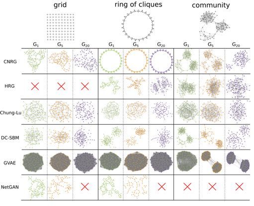
We illustrate some initial results in Figure 7 using three synthetic input graphs with easily-
identifiable visual structure G0 = {a 10 ⇥ 10 grid graph, a 25-node ring of 4-cliques, and a
synthetic graph with 3 well-defined communities}.
Methodology and Evaluation Plan
We consider the following graph models M = {Chung-Lu, degree-corrected SBM (DC-
SBM), Hyperedge Replacement Grammars (HRG), Clustering-based Node Replacement Gram-
mars (CNRG), GVAE, and NetGAN}.
Gi
fit M gen
Gi+1
Qi
repeat
Figure 6: The idea behind the infinity mirror is to iteratively to fit our model M on Gi , use the fitted
parameters Qi to generate the next graph Gi+1 , and repeat with Gi+1 .
11Figure 7: (Best viewed in color.) Plot showing the evolution of various graph models at generations 1, 5,
and 20 (G1 , G5 , G20 ) on three types of synthetic graphs. Red ⇥ indicates model fit failure.
For each combination of input graph G0 and generative model M, we generate 50 indepen-
dent chains of length k = 20 and compute the DeltaCON score [81] comparing G0 and Gk . We
select the chain resulting in the median DeltaCON score, and illustrate G1 , G5 , and G20 (i.e., the
1st , 5th , and 20th generations) in Figure 7 if they exist.
Preliminary Results and Discussions
These initial results show that CNRG can capture and maintain certain structures from the
input graph: on the ring of cliques we see perfect replication, as well as on the first generation
of community, with some marginal degradation as the number of repetitions increases. SBM
performs similarly-well on such structured input. Neither model works particularly well on
grids; CNRG introduces triangles, while SBM creates nodes of degree 1.
HRG fails entirely for grids and does not appear to perform well on the other two graph
types. The Chung-Lu model mimics the degree distribution of the input as we would expect,
but fails to capture the network structure. We can see long chains formed from the grid input
by the last generation, and the output of the other two graph types do not resemble the original
graph. We also see that Chung-Lu fails to preserve the connectivity of the graph, as shown by
the disconnected components in the last generation of each column.
GraphVAE results in overly dense graphs regardless of the input, which obfuscates any topo-
logical structure the input graph had. NetGAN tends to produce sparse, tree-like graphs. This
becomes a problem down the line. The way that NetGAN computes its train/test/validation
split relies on finding a spanning tree on the input graph; when the model is recursively applied
12to its increasingly tree-like outputs, it will eventually fail to find a satisfactory split, causing the
model to fail to fit.
The infinity mirror test we proposed exposes biases in models that might otherwise go unno-
ticed. Future work will determine how best to use this methodology to analyze biases and errors
in graph models.
3.3 Multi-Layer Vertex Replacement Graph Grammars
So far in this proposal, we have restricted ourselves to homogeneous networks, where all the
nodes and edges are identical. In practice, we often deal with networks where individual nodes
and edges have associate attributes. Edges in those cases usually encode a specific connectivity
pattern across a set of nodes. We call such networks heterogeneous, and while researchers have
proposed methods to model such graphs, it remains an open area of research [82–85].
Graph grammars, due to their somewhat simple design, should allow us to adapt previously
used formalisms to a heterogenous setting. However, care must be exercised while doing so, since
it can lead to overfitting the input graph leading to an exponential number of graph rewriting
rules. As the starting point, we will study a specific class of heterogeneous graphs known as
multi-layer graphs [86–88]. The airline network can be thought of as a multi-layer network, with
nodes representing airports, edges representing non-stop flights by an airline, and where each
airline has its own layer. Temporal networks can be thought of as multi-layer networks with
the different time steps represented as different layers. More generally, though the layers can
represent different contexts, and a node u in layer `1 can be connected to a node v in any layer
`2 . So, the edges can be classified into two categories—intra-layer and inter-layer—depending on
whether their endpoints lie on same or different layers.
Multi-layer graphs are usually represented with a pair of tensors, each encoding the intra-
layer and inter-layer connectivity patterns respectively. This idea can be extended to learn a pair
of inter and intra-layer graph grammars. However, while doing so, we should look to preserve
the node correspondence as well as attribute correlations across layers, and not treat the layers
as independent networks.
Evaluation Plan We will adopt a methodology of similar rigor used in the previous papers to
study multi-layer graph grammars. By using a combination of synthetic and real-world multi-
layer graphs obtained from the SNAP, ICON, and Konect databases we will test out the accuracy
of the proposed model(s). This can be achieved by comparing the different distributions asso-
ciated with multi-layer networks as well as studying communities and other mesoscale struc-
tures [89].
134 Summary
In this proposal, we have described that we have done to understand how we can study and
design flexible, interpretable, and scalable graph models by using graph grammars. Furthermore,
by doing so we lay the groundwork for future work in this space, some of which are highlighted
in Section 3. Together, the research in this proposal introduces novel ideas into the fields of
network science, data mining, and graph theory.
4.1 Timeline
Activity Duration
Infinity Mirror Now - May 2020
Stable Graph Grammars Aug - Dec 2020
Attributed Graph Grammars Jan - Dec 2021
Defend Spring 2022
14References
[1] Thomas S Kuhn. The structure of scientific revolutions. University of Chicago press, 2012.
[2] Bruce L Clarke. Theorems on chemical network stability. The Journal of Chemical Physics, 62
(3):773–775, 1975.
[3] Gheorghe Craciun and Casian Pantea. Identifiability of chemical reaction networks. Journal
of Mathematical Chemistry, 44(1):244–259, 2008.
[4] W Ford Doolittle and Eric Bapteste. Pattern pluralism and the tree of life hypothesis. Pro-
ceedings of the National Academy of Sciences, 104(7):2043–2049, 2007.
[5] Stuart A Kauffman. The origins of order: Self organization and selection in evolution. Oxford
University Press, USA, 1993.
[6] David Easley and Jon Kleinberg. Networks, crowds, and markets: Reasoning about a highly
connected world. Cambridge University Press, 2010.
[7] Mark S Granovetter. The strength of weak ties. American journal of sociology, pages 1360–1380,
1973.
[8] Ed Bullmore and Olaf Sporns. Complex brain networks: graph theoretical analysis of struc-
tural and functional systems. Nature Reviews Neuroscience, 10(3):186–198, 2009.
[9] Danielle Smith Bassett and ED Bullmore. Small-world brain networks. The neuroscientist, 12
(6):512–523, 2006.
[10] Bryan Hooi, Hyun Ah Song, Alex Beutel, Neil Shah, Kijung Shin, and Christos Faloutsos.
Fraudar: Bounding graph fraud in the face of camouflage. In Proceedings of the 22nd ACM
SIGKDD International Conference on Knowledge Discovery and Data Mining, pages 895–904,
2016.
[11] Leman Akoglu, Hanghang Tong, and Danai Koutra. Graph based anomaly detection and
description: a survey. Data mining and knowledge discovery, 29(3):626–688, 2015.
[12] Michael Hay, Gerome Miklau, David Jensen, Philipp Weis, and Siddharth Srivastava.
Anonymizing social networks. Computer science department faculty publication series, page
180, 2007.
[13] Gösta Grahne and Jianfei Zhu. Fast algorithms for frequent itemset mining using fp-trees.
TKDE, 17(10):1347–1362, 2005.
[14] Chuntao Jiang, Frans Coenen, and Michele Zito. A survey of frequent subgraph mining
algorithms. The Knowledge Engineering Review, 28(01):75–105, 2013.
[15] Marisa Thoma, Hong Cheng, Arthur Gretton, Jiawei Han, Hans-Peter Kriegel, Alex Smola,
Le Song, Philip S Yu, Xifeng Yan, and Karsten M Borgwardt. Discriminative frequent sub-
graph mining with optimality guarantees. Statistical Analysis and Data Mining, 3(5):302–318,
2010.
[16] Xifeng Yan and Jiawei Han. gspan: Graph-based substructure pattern mining. In ICDM,
pages 721–724. IEEE, 2002.
1[17] Siegfried Nijssen and Joost N Kok. The gaston tool for frequent subgraph mining. Electronic
Notes in Theoretical Computer Science, 127(1):77–87, 2005.
[18] Wenqing Lin, Xiaokui Xiao, and Gabriel Ghinita. Large-scale frequent subgraph mining in
mapreduce. In ICDE, pages 844–855. IEEE, 2014.
[19] Zhao Sun, Hongzhi Wang, Haixun Wang, Bin Shao, and Jianzhong Li. Efficient subgraph
matching on billion node graphs. Proceedings of the VLDB Endowment, 5(9):788–799, 2012.
[20] Nataša Pržulj. Biological network comparison using graphlet degree distribution. Bioinfor-
matics, 23(2):e177–e183, 2007.
[21] Dror Marcus and Yuval Shavitt. Rage–a rapid graphlet enumerator for large networks.
Computer Networks, 56(2):810–819, 2012.
[22] Nesreen K Ahmed, Jennifer Neville, Ryan A Rossi, and Nick Duffield. Efficient graphlet
counting for large networks. In ICDM, pages 1–10. IEEE, 2015.
[23] Paul Erdos and Alfréd Rényi. On the evolution of random graphs. Bull. Inst. Internat. Statist,
38(4):343–347, 1961.
[24] Duncan J Watts and Steven H Strogatz. Collective dynamics of ‘small-world’networks. na-
ture, 393(6684):440–442, 1998.
[25] Albert-László Barabási and Réka Albert. Emergence of scaling in random networks. science,
286(5439):509–512, 1999.
[26] Ginestra Bianconi and A-L Barabási. Competition and multiscaling in evolving networks.
EPL (Europhysics Letters), 54(4):436, 2001.
[27] Erzsébet Ravasz and Albert-László Barabási. Hierarchical organization in complex networks.
Phys. Rev. E, 67(2):026112, 2003.
[28] Petter Holme and Beom Jun Kim. Growing scale-free networks with tunable clustering.
Physical review E, 65(2):026107, 2002.
[29] Andrea Lancichinetti, Santo Fortunato, and Filippo Radicchi. Benchmark graphs for testing
community detection algorithms. Physical review E, 78(4):046110, 2008.
[30] Fan Chung and Linyuan Lu. The average distances in random graphs with given expected
degrees. Proceedings of the National Academy of Sciences, 99(25):15879–15882, 2002.
[31] Joseph J Pfeiffer, Timothy La Fond, Sebastian Moreno, and Jennifer Neville. Fast generation
of large scale social networks while incorporating transitive closures. In SocialCom Workshop
on Privacy, Security, Risk and Trust (PASSAT), pages 154–165. IEEE, 2012.
[32] Stephen Mussmann, John Moore, Joseph J Pfeiffer, and Jennifer Neville III. Assortativity in
chung lu random graph models. In Workshop on Social Network Mining and Analysis, page 3.
ACM, 2014.
[33] Stephen Mussmann, John Moore, Joseph John Pfeiffer III, and Jennifer Neville. Incorporating
assortativity and degree dependence into scalable network models. In AAAI, pages 238–246,
2015.
2[34] Tamara G Kolda, Ali Pinar, Todd Plantenga, and C Seshadhri. A scalable generative graph
model with community structure. SIAM Journal on Scientific Computing, 36(5):C424–C452,
2014.
[35] Brian Karrer and Mark EJ Newman. Stochastic blockmodels and community structure in
networks. Physical review E, 83(1):016107, 2011.
[36] Thorben Funke and Till Becker. Stochastic block models: A comparison of variants and
inference methods. PloS one, 14(4), 2019.
[37] Christopher Aicher, Abigail Z Jacobs, and Aaron Clauset. Adapting the stochastic block
model to edge-weighted networks. arXiv preprint arXiv:1305.5782, 2013.
[38] Daniel B Larremore, Aaron Clauset, and Abigail Z Jacobs. Efficiently inferring community
structure in bipartite networks. Physical Review E, 90(1):012805, 2014.
[39] Tiago P Peixoto. Inferring the mesoscale structure of layered, edge-valued, and time-varying
networks. Physical Review E, 92(4):042807, 2015.
[40] Tiago P Peixoto. Hierarchical block structures and high-resolution model selection in large
networks. Physical Review X, 4(1):011047, 2014.
[41] Garry Robins, Pip Pattison, Yuval Kalish, and Dean Lusher. An introduction to exponential
random graph (p*) models for social networks. Social networks, 29(2):173–191, 2007.
[42] Anna Goldenberg, Alice X Zheng, Stephen E Fienberg, and Edoardo M Airoldi. A survey of
statistical network models. Foundations and Trends in Machine Learning, 2(2):129–233, 2010.
[43] Jure Leskovec, Deepayan Chakrabarti, Jon Kleinberg, Christos Faloutsos, and Zoubin
Ghahramani. Kronecker graphs: An approach to modeling networks. Journal of Machine
Learning Research, 11(Feb):985–1042, 2010.
[44] Jure Leskovec and Christos Faloutsos. Scalable modeling of real graphs using kronecker
multiplication. In ICML, pages 497–504. ACM, 2007.
[45] David F Gleich and Art B Owen. Moment-based estimation of stochastic kronecker graph
parameters. Internet Mathematics, 8(3):232–256, 2012.
[46] Jiaxuan You, Rex Ying, Xiang Ren, William L Hamilton, and Jure Leskovec. Graphrnn: Gen-
erating realistic graphs with deep auto-regressive models. arXiv preprint arXiv:1802.08773,
2018.
[47] Martin Simonovsky and Nikos Komodakis. Graphvae: Towards generation of small graphs
using variational autoencoders. In International Conference on Artificial Neural Networks, pages
412–422. Springer, 2018.
[48] Thomas N Kipf and Max Welling. Variational graph auto-encoders. arXiv preprint
arXiv:1611.07308, 2016.
[49] Yujia Li, Oriol Vinyals, Chris Dyer, Razvan Pascanu, and Peter Battaglia. Learning deep
generative models of graphs. arXiv preprint arXiv:1803.03324, 2018.
[50] Guillaume Salha, Romain Hennequin, and Michalis Vazirgiannis. Simple and effective graph
autoencoders with one-hop linear models. arXiv preprint arXiv:2001.07614, 2020.
3[51] Seongjun Yun, Minbyul Jeong, Raehyun Kim, Jaewoo Kang, and Hyunwoo J Kim. Graph
transformer networks. In Advances in Neural Information Processing Systems, pages 11960–
11970, 2019.
[52] Aleksandar Bojchevski, Oleksandr Shchur, Daniel Zügner, and Stephan Günnemann. Net-
gan: Generating graphs via random walks. arXiv preprint arXiv:1803.00816, 2018.
[53] William C Rounds. Context-free grammars on trees. In Proceedings of the first annual ACM
symposium on Theory of computing, pages 143–148, 1969.
[54] Karl M Schimpf and Jean H Gallier. Tree pushdown automata. Journal of Computer and
System Sciences, 30(1):25–40, 1985.
[55] Salvador Aguinaga, David Chiang, and Tim Weninger. Learning hyperedge replacement
grammars for graph generation. IEEE transactions on pattern analysis and machine intelligence,
41(3):625–638, 2018.
[56] Satyaki Sikdar, Justus Hibshman, and Tim Weninger. Modeling graphs with vertex replace-
ment grammars. In ICDM. IEEE, 2019.
[57] Justus Hibshman, Satyaki Sikdar, and Tim Weninger. Towards interpretable graph modeling
with vertex replacement grammars. In BigData. IEEE, 2019.
[58] Partha Basuchowdhuri, Satyaki Sikdar, Varsha Nagarajan, Khusbu Mishra, Surabhi Gupta,
and Subhashis Majumder. Fast detection of community structures using graph traversal in
social networks. Knowledge and Information Systems, 59(1):1–31, 2019.
[59] Partha Basuchowdhuri, Satyaki Sikdar, Sonu Shreshtha, and Subhashis Majumder. Detecting
community structures in social networks by graph sparsification. In Proceedings of the 3rd
IKDD Conference on Data Science, 2016, pages 1–9, 2016.
[60] Mihael Ankerst, Markus M Breunig, Hans-Peter Kriegel, and Jörg Sander. Optics: ordering
points to identify the clustering structure. ACM Sigmod record, 28(2):49–60, 1999.
[61] Neil Butcher, Trenton Ford, Mark Horeni, Kremer-Herman Nathaniel, Steven Kreig, Brian
Page, Tim Shaffer, Satyaki Sikdar, Famim Talukder, and Tong Zhao. Spectral community
detection. In Peter M. Kogge, editor, A Survey of Graph Kernels, pages 67–75. University of
Notre Dame, 2019. URL https://dx.doi.org/doi:10.7274/r0-e7wb-da60.
[62] Neil Butcher, Trenton Ford, Mark Horeni, Kremer-Herman Nathaniel, Steven Kreig, Brian
Page, Tim Shaffer, Satyaki Sikdar, Famim Talukder, and Tong Zhao. Networkx graph library.
In Peter M. Kogge, editor, A Survey of Graph Processing Paradigms, pages 67–70. University of
Notre Dame, 2019. URL https://dx.doi.org/doi:10.7274/r0-z6dc-9c71.
[63] Corey Pennycuff, Satyaki Sikdar, Catalina Vajiac, David Chiang, and Tim Weninger. Syn-
chronous hyperedge replacement graph grammars. In International Conference on Graph
Transformation, pages 20–36. Springer, 2018.
[64] Grzegorz Rozenberg. Handbook of Graph Grammars and Comp., volume 1. World scientific,
1997.
[65] Vincent D Blondel, Jean-Loup Guillaume, Renaud Lambiotte, and Etienne Lefebvre. Fast
unfolding of communities in large networks. Journal of statistical mechanics: theory and exper-
iment, 2008(10):P10008, 2008.
4[66] Andrew Y Ng, Michael I Jordan, and Yair Weiss. On spectral clustering: Analysis and an
algorithm. In NeurIPS, pages 849–856, 2002.
[67] Diane J Cook and Lawrence B Holder. Substructure discovery using minimum description
length and background knowledge. Journal of Artificial Intelligence Research, 1:231–255, 1993.
[68] Nataša Pržulj. Biological network comparison using graphlet degree distribution. Bioinfor-
matics, 23(2):e177–e183, 2007.
[69] V. A. Traag, L. Waltman, and N. J. van Eck. From Louvain to Leiden: guaranteeing well-
connected communities. Scientific Reports, 9(1):5233, March 2019. ISSN 2045-2322. doi: 10.
1038/s41598-019-41695-z. URL https://doi.org/10.1038/s41598-019-41695-z.
[70] Martin Rosvall, Daniel Axelsson, and Carl T Bergstrom. The map equation. The European
Physical Journal Special Topics, 178(1):13–23, 2009.
[71] Benjamin H Good, Yves-Alexandre De Montjoye, and Aaron Clauset. Performance of mod-
ularity maximization in practical contexts. Physical Review E, 81(4):046106, 2010.
[72] Aditya Tandon, Aiiad Albeshri, Vijey Thayananthan, Wadee Alhalabi, and Santo Fortunato.
Fast consensus clustering in complex networks. Physical Review E, 99(4):042301, 2019.
[73] Andrea Lancichinetti and Santo Fortunato. Consensus clustering in complex networks. Sci-
entific reports, 2:336, 2012.
[74] Kun Zhan, Feiping Nie, Jing Wang, and Yi Yang. Multiview consensus graph clustering.
IEEE Transactions on Image Processing, 28(3):1261–1270, 2018.
[75] Nam Nguyen and Rich Caruana. Consensus clusterings. In Seventh IEEE International Con-
ference on Data Mining (ICDM 2007), pages 607–612. IEEE, 2007.
[76] Li Zheng, Tao Li, and Chris Ding. Hierarchical ensemble clustering. In 2010 IEEE Interna-
tional Conference on Data Mining, pages 1199–1204. IEEE, 2010.
[77] Ji Qi, Hong Luo, and Bailin Hao. Cvtree: a phylogenetic tree reconstruction tool based on
whole genomes. Nucleic acids research, 32(suppl 2):W45–W47, 2004.
[78] Rui Yang, Panos Kalnis, and Anthony KH Tung. Similarity evaluation on tree-structured
data. In SIGMOD, pages 754–765. ACM, 2005.
[79] Juris Hartmanis. Context-free languages and turing machine computations. In Proceedings
of Symposia in Applied Mathematics, volume 19, pages 42–51, 1967.
[80] Karim Lari and Steve J Young. The estimation of stochastic context-free grammars using the
inside-outside algorithm. Computer speech & language, 4(1):35–56, 1990.
[81] Danai Koutra, Neil Shah, Joshua T Vogelstein, Brian Gallagher, and Christos Faloutsos.
Deltacon: principled massive-graph similarity function with attribution. ACM Trans. on
Knowledge Discovery from Data, 10(3):28, 2016.
[82] Joseph J Pfeiffer III, Sebastian Moreno, Timothy La Fond, Jennifer Neville, and Brian Gal-
lagher. Attributed graph models: Modeling network structure with correlated attributes. In
Proceedings of the 23rd international conference on World wide web, pages 831–842, 2014.
5[83] Cécile Bothorel, Juan David Cruz, Matteo Magnani, and Barbora Micenkova. Clustering
attributed graphs: models, measures and methods. Network Science, 3(3):408–444, 2015.
[84] Natalie Stanley, Thomas Bonacci, Roland Kwitt, Marc Niethammer, and Peter J Mucha.
Stochastic block models with multiple continuous attributes. Applied Network Science, 4(1):
1–22, 2019.
[85] Jacek Kukluk, Lawrence Holder, and Diane Cook. Inferring graph grammars by detecting
overlap in frequent subgraphs. International Journal of Applied Mathematics and Computer
Science, 18(2):241–250, 2008.
[86] Mikko Kivelä, Alex Arenas, Marc Barthelemy, James P Gleeson, Yamir Moreno, and Ma-
son A Porter. Multilayer networks. Journal of complex networks, 2(3):203–271, 2014.
[87] Stefano Boccaletti, Ginestra Bianconi, Regino Criado, Charo I Del Genio, Jesús Gómez-
Gardenes, Miguel Romance, Irene Sendina-Nadal, Zhen Wang, and Massimiliano Zanin.
The structure and dynamics of multilayer networks. Physics Reports, 544(1):1–122, 2014.
[88] Alberto Aleta and Yamir Moreno. Multilayer networks in a nutshell. Annual Review of
Condensed Matter Physics, 10:45–62, 2019.
[89] Peter J Mucha, Thomas Richardson, Kevin Macon, Mason A Porter, and Jukka-Pekka On-
nela. Community structure in time-dependent, multiscale, and multiplex networks. science,
328(5980):876–878, 2010.
1You can also read