Estimation of unsteady hydromagnetic Williamson fluid flow in a radiative surface through numerical and artificial neural network modeling
←
→
Page content transcription
If your browser does not render page correctly, please read the page content below
www.nature.com/scientificreports

                OPEN              Estimation of unsteady
                                  hydromagnetic Williamson
                                  fluid flow in a radiative surface
                                  through numerical and artificial
                                  neural network modeling
                                  Anum Shafiq1, Andaç Batur Çolak2, Tabassum Naz Sindhu3, Qasem M. Al‑Mdallal4* &
                                  T. Abdeljawad5

                                  In current investigation, a novel implementation of intelligent numerical computing solver based on
                                  multi-layer perceptron (MLP) feed-forward back-propagation artificial neural networks (ANN) with
                                  the Levenberg–Marquard algorithm is provided to interpret heat generation/absorption and radiation
                                  phenomenon in unsteady electrically conducting Williamson liquid flow along porous stretching
                                  surface. Heat phenomenon is investigated by taking convective boundary condition along with
                                  both velocity and thermal slip phenomena. The original nonlinear coupled PDEs representing the
                                  fluidic model are transformed to an analogous nonlinear ODEs system via incorporating appropriate
                                  transformations. A data set for proposed MLP-ANN is generated for various scenarios of fluidic model
                                  by variation of involved pertinent parameters via Galerkin weighted residual method (GWRM). In order
                                  to predict the (MLP) values, a multi-layer perceptron (MLP) artificial neural network (ANN) has been
                                  developed. There are 10 neurons in hidden layer of feed forward (FF) back propagation (BP) network
                                  model. The predictive performance of ANN model has been analyzed by comparing the results
                                  obtained from the ANN model using Levenberg-Marquard algorithm as the training algorithm with
                                  the target values. When the obtained Mean Square Error (MSE), Coefficient of Determination (R) and
                                  error rate values have been analyzed, it has been concluded that the ANN model can predict SFC and
                                  NN values with high accuracy. According to the findings of current analysis, ANN approach is accurate,
                                  effective and conveniently applicable for simulating the slip flow of Williamson fluid towards the
                                  stretching plate with heat generation/absorption. The obtained results showed that ANNs are an ideal
                                  tool that can be used to predict Skin Friction Coefficients and Nusselt Number values.

                                 Nomenclature
                                 T̂ 	Fluid’s temperature
                                 T̂w	Wall’s temperature
                                 K̃ 	Fluid’s thermal conductivity
                                 Ec	Eckert number
                                 σ̃ ∗	Stefan–Boltzmann constant
                                 v̂, û,	Velocity components
                                 Pr	Prandtl number
                                 α	thermal slip number
                                 M12	Magnetic parameter
                                 R1	Radiation parameter
                                 We	Weissenberg number

                                  1
                                   School of Mathematics and Statistics, Nanjing University of Information Science and Technology, Nanjing 210044,
                                  China. 2Mechanical Engineering Department, Niğde Ömer Halisdemir University, Niğde, Turkey. 3Department of
                                  Statistics, Quaid- i- Azam University 45320, Islamabad 44000, Pakistan. 4Department of Mathematical Sciences,
                                  UAE University, P.O. Box 15551, Al‑Ain, United Arab Emirates. 5Department of Mathematics and General Sciences,
                                  Prince Sultan University, Riyadh, Saudi Arabia. *email: q.almdallal@uaeu.ac.ae

Scientific Reports |   (2021) 11:14509               | https://doi.org/10.1038/s41598-021-93790-9                                               1

                                                                                                                                           Vol.:(0123456789)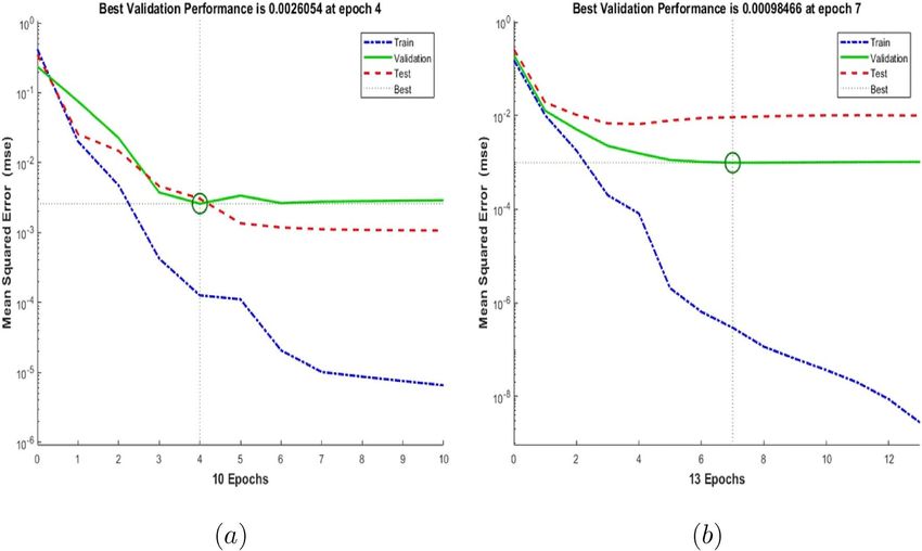
www.nature.com/scientificreports/
Ŵ̃ Time constant
Ũw Variable stretching velocity
c̃p Specific heat
Q1 Heat generation parameter
Bi Biot number
T̂∞ Ambient fluid’s temperature
γ1 Velocity slip number
E1 Local electric number
A1 Suction/injection coefficient
S1 Unsteadiness parameter
R̃(x) Residual function
Greek symbols
q̃r∗ Radiative heat flux
ρ̃0∗ Fluid density
σ̌ ∗ Stefan–Boltzmann constant
ν Kinematic viscosity
̟ Angel of inclination
ǩ1 Mean absorption coefficient
ρ̃0∗ Density of fluid
Abbreviations
MLP Multi-layer perceptron
ANN Artificial neural network
GWRM Galerkin weighted residual method
GLF Gauss–Laguerre formula
FF Feed forward
BP Back propagation
MSE Mean square error
FFBP Feed-forward back-propagation
The importance of non-Newtonian substances in variety of mechanical, chemical processes and implementations
in engineering is quite evident. The uses of these substances are significant in medicines, surfactants, petroleum
engineering, blood and many other. However thoroughly analyzing the subgroups of non-Newtonian liquids,
Williamson liquid is also categorized into these substances owing to classical characteristics of shear thinning/
thickening. Having these distinct motivations in mind, several researchers adopt this model with different flow
aspects and configurations1–7.
Thermal radiation performs a pivotal part in engineering and physics particularly in high temperature process
and space technology. Most of these uses contain gas turbines, the polymer manufacturing industry, nuclear
power plants and different propulsion systems for rocket, spacecraft, aircraft and satellite. Hashim et al.8 con-
centrated on radiation impacts on Williamson liquid owing to an expanding/contracting cylinder containing
nanomaterials. In9, the impact of non-linear radiation on time dependent flow of a Williamson liquid via heat
source/sink was explored. The MHD boundary layer (BL), chemical reacting and heat generating Nano-fluidic
flow towards a moving radiative wedge examined in10. Hayat et al.11 explored the hydromagnetic boundary layer
flow of Williamson liquid under the influence of Ohmic dissipation and radiation. For more details one can read
the suggested reference12–17.
Magnetic fields exist anywhere in nature, so magnetohydrodynamic (MHD) mechanisms must arise when
liquid conduction is accessible. It also has several engineering uses like aeronautics field, stellar/planetary magne-
tospheres, cosmic fluid dynamics, solar physics, MHD generators, chemical engineering, electronics, construction
of turbines, MHD accelerators and many more. Whenever a magnetic field is added to an electrically conduct-
ing moving liquid, both electric and magnetic fields are induced. These fields communicate among each other,
generating a body force identified as the Lorentz force, that slows down fluid movement. Recently numerous
sleuths18–24 investigated on MHD by different fluid flows. In several practical uses, like non-mechanical MHD
micropumps, the analysis of Magnetohydrodynamic slip flow demonstrated favourable performance. Reza-E-
Rabbi et al.25 detailed the heat and mass transfer analysis of Casson nanofluid flow passing through a stretching
layer with magnetohydrodynamic (MHD), thermal radiation, and chemical reaction effects. Boundary layer
approximations formed the main equations, namely the momentum, energy and diffusion equilibrium equations
with respect to time. The effect of various physical parameters on the momentum and thermal boundary layers
is discussed and graphically illustrated together with the concentration profiles. Arifuzzaman et al.26 analyzed
the heat and mass transfer properties of the natural convective hydromagnetic flow of the fluid with fourth order
radiation originating from the vertical porous plate. The impression of heat generation by nonlinear sequential
chemical reaction and thermal diffusion is also taken into account. The combined fundamental equations are
transformed into a dimensionless arrangement by explicitly applying the finite difference scheme. As a result of
the study, it was stated that the velocity fields started to decrease as the temperature of the fluid increased, but
the opposite situation emerged for the temperature fields. Arifuzzaman et al.27 analyzed the appearance of nano-
sized particles and the hydrodynamic flow behavior of Casson and Maxwell fluids with multiphase radiation.
Scientific Reports | (2021) 11:14509 | https://doi.org/10.1038/s41598-021-93790-9 2
Vol:.(1234567890)
www.nature.com/scientificreports/
Figure 1. Physical configuration of the flow model.
First, the time-dependent governing equations are solved computationally using finite difference discretization
methods, and then convergence analysis is performed with the stabilization of the numerical approach. Finally,
impressions of various relevant parameters are schematically depicted along with tabular analysis over diversified
flow fields. The thermal and bulk properties found are significantly improved mostly in the case of Maxwell fluid.
For numerical validation, some comparisons with previous studies were also shown and satisfactory agreement
was observed. A partial slip would be utilized for stationary as well as moving boundary whenever a particulate
liquid has been employed e.g. suspensions, emulsions, polymer solutions and foams. Several investigators have
studied the significance of slip velocity influence in various flow types, i ncluding28–31. The hydromagnetic BL slip
flow of a Maxwell nanoliquid over an exponentially expanding surface under convective boundary condition
was examined by Reddy et al.32. The consequences of multiple slips on the flow of magneto-Carreau liquid over
the wedge with chemically reactive species were studied by Khan and H ashim33 and the increase in shear stress
and fluid velocity was investigated by increasing the magnetic parameter whereas decreasing the temperature
and concentration fields.
To the best of researchers’ information, no studies has yet been made to examine the electro-hydrodynamic
slip flow of Williamson fluid towards a permeable stretched surface with heat generation/absorption via ANN
model. The literature summary demonstrates that in providing solutions to nonlinear issues, the ANN models
have been very effective. Thus, the novelty of current study centered on usefulness of ANN procedure for bound-
ary layer slip flow (BLSF) of Williamson fluid flow towards a stretching sheet by taking convective boundary
condition and heat absorption/generation. The influences of related parameters on features of flow and heat
transport are evaluated in this analysis and numerical outcomes are given in connection with the outcomes of
ANN procedure.
Present study has structured as given: Section 2 includes mathematical problem formulation. Galerkin
weighted residual method (GWRM) is given in Section 3. Section 4 includes the significance of ANN technique
and BPA (Back Propagation algorithm). Section 5 deals with the result and discussion and Section 6 ends up
with final findings .
Problem development
Two dimensional incompressible unsteady electrically conducting BLF of Williamson liquid towards a porous
stretched surface under velocity as well as thermal slip condition is considered. The x-axis is considered towards
extending surface in direction of movement whereas y-axis is taking perpendicular as shown in Fig. 1a. The
current fluidic system also incorporates viscous dissipation, heat source/sink and radiation effects. The flow
area is displayed by considering uniform transverse magnetic B̄ and electric Ē fields and known as the electri-
cally conducting
fluid. Remember that magnetic field is poorer than electric field and magnetic field follows
J ¯=σ Ē + V̄ × B̄ Ohm’s law, where J̄ represnts Joule current, σ represents electrical conductivity and V̄ rep-
resents fluid velocity. The related flow equations while obtaining BL approximations takes the following form
∂ û ∂ v̂
+ =0, (1)
∂ x̂ ∂ ŷ
∂ û ∂ û ∂ û ∂ 2 û ∂ û ∂ 2 û σ̃
+ ∗ sin2 (̟ ) Ẽ0 B̃0 − B̃02 û , (2)
+ v̂ + û =ν 2 + 2ν Ŵ̃
∂t ∂ ŷ ∂ x̂ ∂ ŷ ∂ ŷ ∂ ŷ 2 ρ̃0
Scientific Reports | (2021) 11:14509 | https://doi.org/10.1038/s41598-021-93790-9 3
Vol.:(0123456789)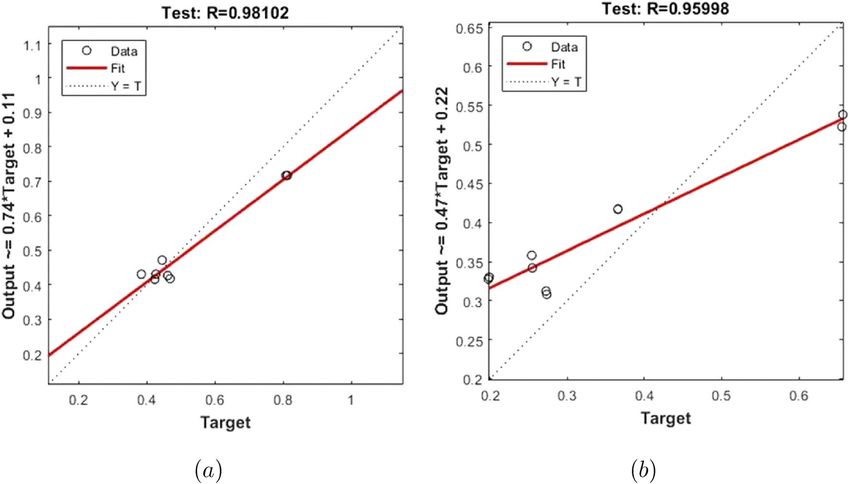
www.nature.com/scientificreports/
2
3
∂ T̂ ∂ T̂ ∂ T̂ ∂ 2 T̂ ∗ ∂ û ∂ û 2
ρ̃0∗ c̃p ∗
+ σ̃ sin2 (̟ ) ûB̃0 − Ẽ0
+ û + v̂ =K̃ + µ̃0 + µ̃0 Ŵ̃
∂t ∂ x̂ ∂ ŷ ∂ ŷ 2 ∂ ŷ ∂ ŷ
(3)
∂ q̃∗
− r + Q̃0 T̂ − T̂∞ ,
∂ ŷ
Here velocity components û and v̂ are in x̂ and ŷ directions respectively, fluid density is ρ̃0∗, thermal conductiv-
ity is K̃ , fluid temperature is T̂ , specific heat is c̃p, kinematic viscosity is ν , time constant is Ŵ̃, angel of inclination
is ̟ and radiative heat flux is q̃r∗. By using the approximation of Rosseland, we have
4σ̌ ∗ ∂ T̂ 4
q̃r∗ = − , (4)
3ǩ1 ∂ ŷ
in which σ̌ ∗ defines Stefan-Boltzmann constant and ǩ1 defines mean absorption coefficient. Employing Taylor’s
series approximation, T̂ 4 ∼ = 4T̂∞ 3 T̂ − 3T̂ 4 , where ambient temperature is T̂ and Eq. (3) becomes
∞ ∞
∂ û 2
3
16σ̌ ∗ T̂∞3 ∂ 2 T̂
∂ T̂ ∂ T̂ ∂ T̂ ∂ û
ρ̃0∗ c̃p + v̂ + û = + K̃ + µ0 + µ0 Ŵ
∂t ∂ ŷ ∂ x̂ 3k̃1 ∂ ŷ 2 ∂ ŷ ∂ ŷ
(5)
2
2
+ σ̃ sin (̟ ) ûB̃0 − Ẽ0 + Q̃0 T̂ − T̂∞ .
with
� � � � � �2
� � ∂ û x̂, 0 ∂ û x̂, 0
û x̂, 0 =L1 µ0 +Ŵ + Ũw ,
∂ ŷ ∂ ŷ
� � ν0 ∂ T̂(x̂, 0) � � ∂ T̂(x̂, 0) (6)
v̂ x̂, 0 =Ṽw = − 1/2
, −k̃f = h̃f T̂w − T̂ + L2 ,
(1 − c1 t) ∂ ŷ ∂ ŷ
� � � �
û x̂, ŷ → ∞ → 0, T̂ x̂, ŷ → ∞ → T̂∞ ,
and Ṽw̃ is
ν0
Ṽw̃ = − . (7)
(1 − c1 t)1/2
including suction/injection Ṽw̃ > 0/Ṽw̃ < 0 . Furthermore,
This
defines the mass transport on the surface
Ũw x̂, t is variable stretching velocity and T̂w x̂, t is variable wall temperature are as follows
a1 x̂ a1 x̂
(8)
Ũw x̂, t = , T̂w x̂, t = T̂∞ + T̂0 ,
1 − c1 t 2ν(1 − c1 t)2
where rate constants are a1 and c1 with a1 > 0 and c1 ≥ 0 (i.e. c1 t < 1). Appropriate transformation are consid-
ered as
Ũw T̂ − T̂∞
ξ= y, ψ = ν x̂ Ũw F(ξ ), θ (ξ ) = , (9)
x̂ν T̂w − T̂∞
with
∂ψ ∂ψ
û = , v̂ = − . (10)
∂ ŷ ∂ x̂
Eq. (1) is identically satisfied and Eqs. (2), (5) and (6) becomes
1
F ′′′ − F ′2 + FF ′′ − S1 F ′ + ξ F ′′ + 2We F ′′ F ′′′ + M12 sin2 (̟ ) E1 − F ′ = 0, (11)
2
4 S1
′
1 + R1 θ ′′ + Pr Ec F ′′2 − Pr F ′ θ − θ ′ F +
ξ θ +4θ
3 2 (12)
′′3 2 2
′ 2
+We Pr Ec F + M1 Pr Ec sin (̟ ) F − E1 + Pr Q1 θ = 0,
2
F (0) =A1 , F ′ (0) = 1 + γ1 F ′′ (0) + We F ′′ (0) , F ′ (ξ → ∞) → 0,
Bi [1 − θ(0)] (13)
θ ′ (0) = − , θ(ξ → ∞) → 0,
1+α
Scientific Reports | (2021) 11:14509 | https://doi.org/10.1038/s41598-021-93790-9 4
Vol:.(1234567890)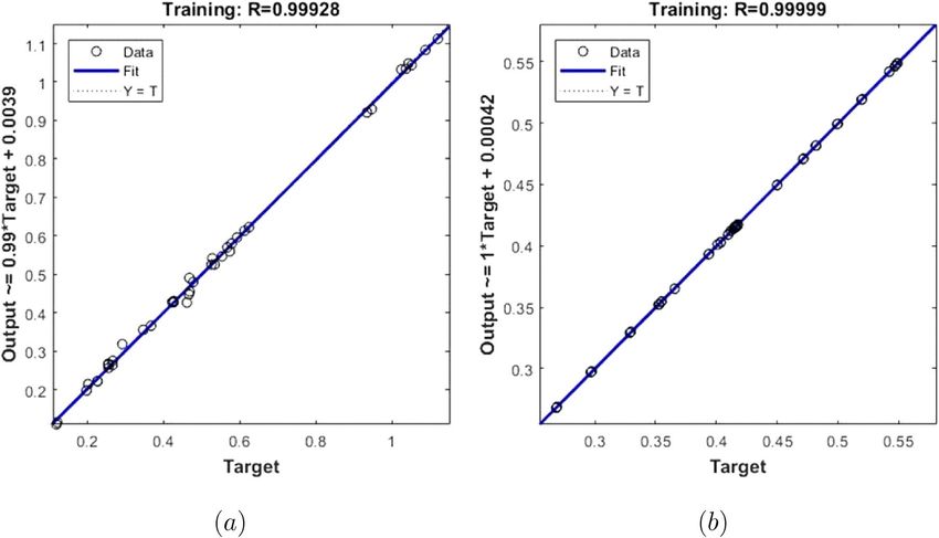
www.nature.com/scientificreports/
σ B̃02 (1−c1 t)
where We = Ŵ Ũw a1
ν(1−c1 t) represents Weissenberg number, M12 = ρ̃0∗ a1 represents magnetic number,
Ẽ0 (1−c1 t)
E1 = represents local electric number, A1 = √ν0
aν
represents suction/injuction parameter, S1 = c1
a1 rep-
B̃0 a1 x̂
4σ̌ ∗ T̂∞
3
resents unsteadiness parameter, γ1 = µ0 L1 a1
ν(1−c1 t) represents velocity slip number, R1 = represents
k∗ K̃
µ c̃
radiation parameter, Pr = 0 p represents Prandtl number, α = L2 represents the thermal slip number,
K̃ k̃f
h̃
Bi = f ν x̂
defines Biot number, Q1 = Q̃0ρ̃(1−c
∗ c̃ a
1 t)
defines the heat generation/ absorption parameter and
k̃f Ũw p 1
0
2
Ec = Ũw
represents the Eckert number.
c̃p T̂w −T̂∞
Expression of skin friction coefficient is
2
µ0 ∂∂ ûŷ + Ŵ ∂∂ ûŷ
τw ŷ = 0
C̃F = = , (14)
∗
ρ Ũw2 ρ ∗ Ũw2
1
Rex̂ C̃F = F ′′ (0) + We F ′′2 (0) .
2
Expression of local Nusselt number (LNN) is
16σ ∗ T̃∞
3
∂ T̃
x̂ 3k1 + K̃ ∂ ŷ
ŷ = 0
x̂ qw
Nux̂ =
=−
,
K̃ T̂w − T̂∞ K̃ T̂w − T̂∞ (15)
4
Re−1/2
x Nu x̂ = − 1 + R1 θ ′ (0).
3
Galerkin weighted residual method (GWRM)
GWRM is an effective method for calculating solutions of nonlinear BVP (boundary value problems). It com-
prises the following main steps: (1) In differential equations, the unknown dependent functions are initially
considered to be linear combinations of form or trial functions containing unknown coefficients. (2) Such sup-
posed solutions are incorporated into equations that contains residuals. (3) The errors are forced to be as small
utilizing certain weight functions, therefore found unknown coefficients. The key characteristics that make this
procedure (GWRM) appealing are (a) The ease of handling BVPs relating semi-infinite range. (b) It has high
precision, performance and quick convergence. (c) the associated range within 0 and ∞ is directly minimized.
Therefore, we utilized GWRM to find the solution of governing differential system (11–12) with (13). GWRM
procedures to seek an approximate solution as follows
F(x) + L̃(χ(x)) = 0 in D̃0 , (16)
here unknown dependent variable is χ(x), independent function is F(x) in domain D̃0 and differential operator
is L̃. An approximate solution
n
χ(x) = χ0 + ak χk (x), (17)
k=1
is defined in fashion that it ensures the specified boundary conditions. Replacing Eq. (17) into Eq. (16) emanated
in R̃(x).R̃(x) (residual function) is reduced as little as possible in D̃0 by putting the integral of product of χk (x)
(weight functions) and R̃(x) over whole D̃0 equal to zero for k ≥ 0, n.
R̃(x)χk (x)dx = 0, k = 0, 1, ..., n. (18)
D
Gauss–Laguerre formula is employed to integrate every equations in (18) to achieve set of algebraic systems since
boundary condition varies from zero to infinity. The ak values are gained via solving the consequent algebraic
systems.
Gauss–Laguerre formula (GLF). GLF is employed as given below34:
∞
n
e−x F(x)dx ≈ Bk F(xk ), (19)
0 k=1
here Bk coefficients have been specified as35
1 ∞ e−x L̃n (x) (n!)2
Bk = dx =
2 , (20)
L̃n′ (xk ) 0 x − xk xk L̃n′ (xk )
and xk are the zeros of nth Laguerre polynomial
Scientific Reports | (2021) 11:14509 | https://doi.org/10.1038/s41598-021-93790-9 5
Vol.:(0123456789)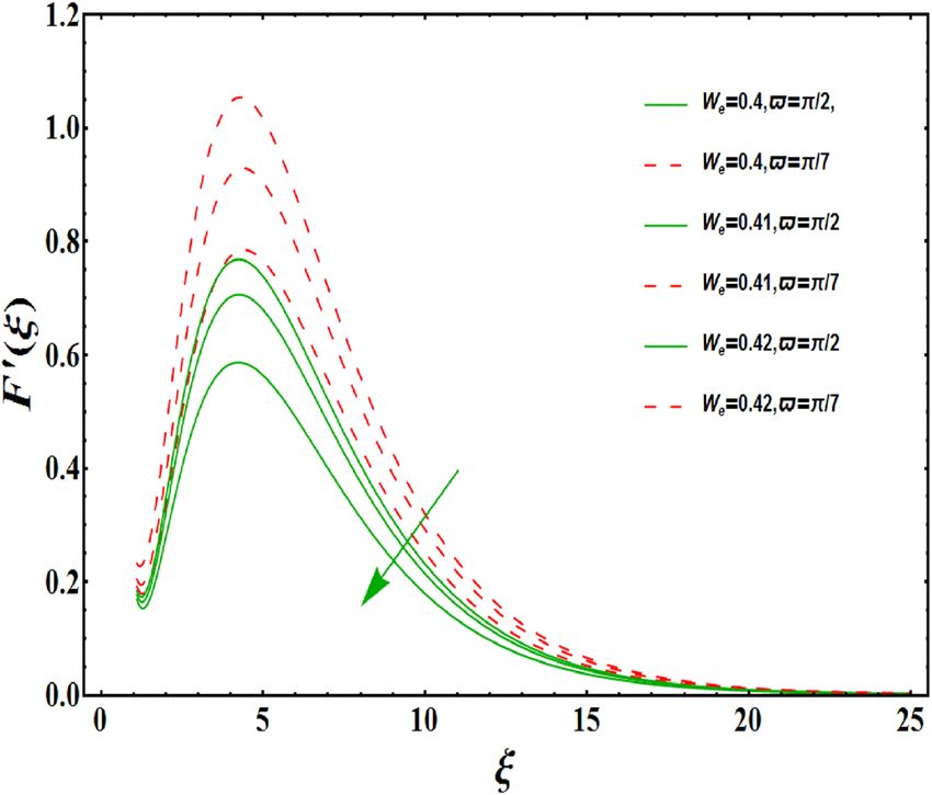
www.nature.com/scientificreports/
d n −x n
L̃n = ex e x . (21)
dx n
For n = 10, Table 1 displays xk values and relating Bk values.
Application of GWRM’s to current problem. Using GWRM, the assumed solutions of F(ξ ) and θ(ξ ) are
considered as given below34
Ñ Ñ
iξ kξ
F(ξ ) = ai e− 3 , θ (ξ ) = bk e− 3 . (22)
i=0 k=1
Selecting Ñ = 15, substituted Eq. (22) into Eq. (13), to atain
− A + a0 + a1 + a2 + a3 + a4 + a5 + a6 + a7 + a8 + a9 + a10 + a11
(23)
+a12 + a13 + a14 + a15 = 0,
a1 2a2 4a4 5a5 7a7 8a8 10a10
−1− − − a3 − − − 2a6 − − − 3a9 −
3 3 3 3 3 3 3
11a11 13a13 14a14
− − 4a12 − − − 5a15 −
3 3 3
a1 4a2 16a4 25a5 49a7 64a8
γ1 + + a3 + + + 4a6 + + + 9a9
9 9 9 9 9 9
(24)
100a10 121a11 169a13 196a14
+ + + 16a12 + + + 25a15
9 9 9 9
a1 4a2 16a4 25a5 49a7 64a8
+ We + + a3 + + + 4a6 + + + 9a9
9 9 9 9 9 9
2
100a10 121a11 169a13 196a14
+ + + 16a12 + + + 25a15 = 0,
9 9 9 9
b1 2b2 4b4 5b5 7b7 8b8 10b10
− − − b3 − − − 2b6 − − − 3b9 −
3 3 3 3 3 3 3
11b11 13b13 14b14 Bi (25)
− − 4b12 − − − 5b15 + {1 − b1 − b2 − b3
3 3 3 1+α
−b4 − b5 − b6 − b7 − b8 − b9 − b10 − b11 − b12 − b13 − b14 − b15 } = 0.
The boundary conditions at infinity in Eq. (13) are automatically satisfied. Putting Eq. (22) into Eqs. (11) and
(12) occurred in R̃F (ai , ξ ) and R̃θ (ai , bk , ξ ) for i = 0, 1, · · iξ· , 15, k =kξ1, 2, · · · , 15. First, minimize residual by taking
integral of product of residual and weight functions e− 3 and e− 3 , for k = 1, 2, . . . , Ñ − 1, i = 0, 1, . . . , Ñ − 2
to zero, i.e.
∞ ∞
iξ kξ
R̃F (ai , ξ ) e− 3 dξ = 0, R̃θ (ai , bk , ξ ) e− 3 dξ = 0, (26)
0 0
together with Eqs. (23–25) produce 2Ñ + 1 nonlinear algebraic systems with 2Ñ + 1 unknown coefficients (ai , bk )
and then solved via MATHEMATICA to get ai and bk.
Neural network modeling
Due to the difficulties of experimental studies, long time and cost, many researchers have worked on numerical
modeling and derivation of mathematical correlations. Misidentification and modeling of experimental and
theoretical data may cause errors in the results obtained from the simulation study. In addition, there are vari-
ous difficulties in modeling nonlinear and non-linear mathematical functions with traditional t ools36. Artificial
neural networks (ANN), which were developed on the basis of the biological working principle of the human
brain, have been one of mathematical measures that are frequently utilized by i nvestigators37. ANNs started to
be used in the middle of the twentieth century. They have a wide range of applications due to their fastness,
flexibility, learning algorithms, and tolerance to e rrors38,39. Thanks to these important advantages, ANNs have
recently become tools that are frequently used in various fields such as medicine and business as well as many
different engineering applications40–44. One of the most frequently used models among ANN models is MLP
network model, that has a feed-forward back-propagation (FFBP) s tructure45,46. An MLP network has an input
layer where input parameters are defined, at least one hidden and one output layer, where predictive values are
gained. The hidden layer contains processing elements called neurons, and each layer is connected to the other
with a transfer function. Optimizing the data to be used in training of ANN is one of the important parameters
affecting the prediction accuracy of ANN. For this reason, the data used in ANN models should be grouped and
optimized ideally47. In this study, two different ANN models have been designed in order to predict SFC and
NN. The data set used in both ANN models is divided into three parts, which are frequently preferred by the
Scientific Reports | (2021) 11:14509 | https://doi.org/10.1038/s41598-021-93790-9 6
Vol:.(1234567890)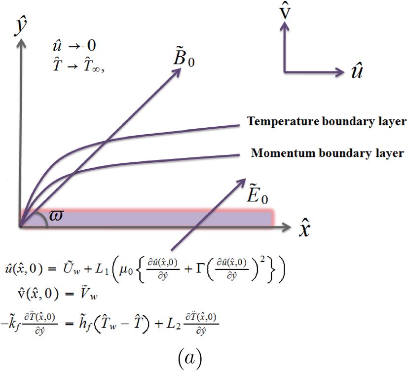
www.nature.com/scientificreports/
Figure 2. The basic structures of the ANN models (a) SFCs (b) NN.
researchers. 70% of the data have been used for training, 15% for validation and 15% for testing48. In the input
layer of the ANN model designed for SFC prediction, We , A, S1 , M1 , E1 and γ1 values have been defined as input
parameters, and the skin friction coefficient value has been predicted at output layer. In MLP network model,
which has been designed with a total of 28 data sets, 20 of data have been used for the training phase, 4 for the
validation phase and 4 for the test phase. In ANN model developed for prediction of NN; M1 , E1 , R1 , Pr , Ec , Q1 ,
Bi and α values are defined as input parameters and Nusselt Number is predicted at output layer. In ANN model
using a total of 33 data sets, 25 of data have been used for training, 5 for validation, and 5 for testing. There is no
exact methodology for determining the number of neurons to be used in A NNs49. For this reason, both ANN
models have been developed with different neuron numbers and their performances have been analyzed. By
evaluating the obtained results, 10 neurons have been used in the hidden layers of both ANN models. The basic
structures of the ANN models developed are shown in Fig. 2a,b.
In the developed ANN models, the Levenberg–Marquardt algorithm, which is one of the powerful algorithms
widely preferred in the literature, has been used as the training algorithm50. In the hidden layer of ANN models,
Tan-Sig function is used as the transfer function and Purelin functions in the output layer51. The transfer func-
tions utilized is provided as:
1
f˜ (x) = , (27)
1 + e−x
purelin(x) =x, (28)
Mean Square Error (MSE), Coefficient of Determination (R) parameters have been used for performance analysis
of the developed MLP network model. In addition, the error rates between values attained from ANN model and
the target values have also been calculated and analyzed. The equations used in the calculation of performance
parameters are given b elow52:
N
1
2
MSE = Xexp (i) − XANN(i) , (29)
N
i=1
N 2
Xexp (i) − XANN(i)
R =
1 − i=1
N 2 , (30)
i=1 Xexp (i)
Scientific Reports | (2021) 11:14509 | https://doi.org/10.1038/s41598-021-93790-9 7
Vol.:(0123456789)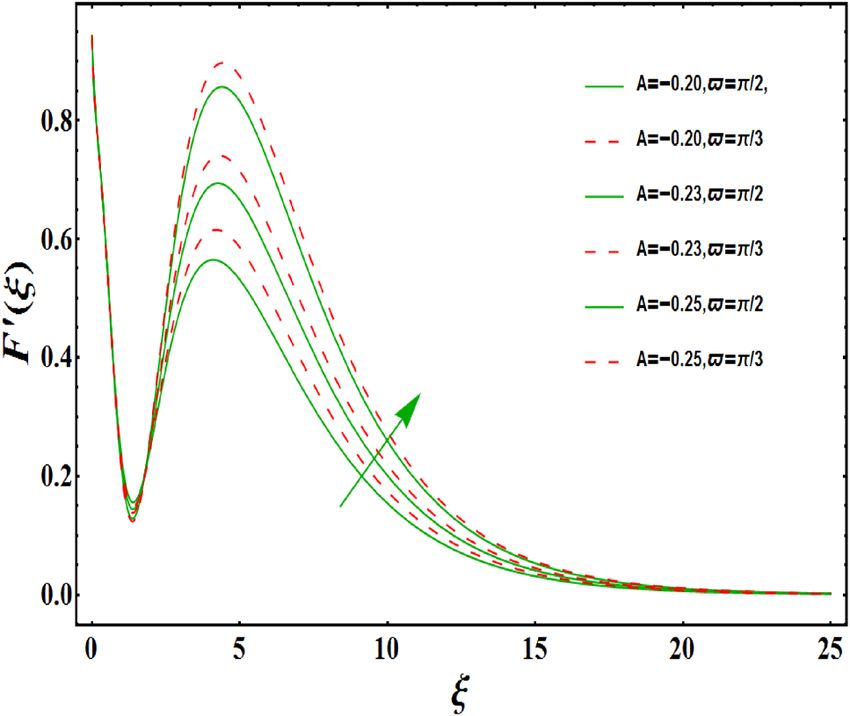
www.nature.com/scientificreports/

                                            Figure 3.  Minimized redidual error R̃F , R̃θ .


                                            Figure 4.  Comparison of the velocity and temperature profiles attained via SCM and GWRM.


                                                                                                    Xexp − XANN
                                                                                   Error Rate(%) =                × 100.                                          (31)
                                                                                                        Xexp

                                            Results and discussion
                                            The GWRM method has been utilized to compute numerical simulation of temperature and velocity fields
                                            within boundary layer for various values of related physical parameters. We explore structural features of all
                                            associated dimensionless parameters on velocity F ′ (ξ ) and temperature θ (ξ ) fields, that are portrayed through
                                            Figs. 5, 6, 7, 8, 9, 10, 11, 12, 13 14 and 15. For the leading variables, we gave default values as: A = 0.4 = M1;
                                            S1 = 0.3 = R1 ; Q1 = We = 0.5 = Ec = E1 ; Pr = 1; γ1 = α = 0.2 = Bi ; during the entire computations unless
                                            otherwise mentioned. The map of R̃F (ai , ξ ) and R̃θ (ai , bk , ξ ) are displayed in Fig. 3. It is noted that residuals in
                                            the range (0 − ∞) are reduced. Further, to see the reliability of the approach employed, a simulation study is
                                            presented. This is obtained by analyzing graphical findings of dimensionless velocity and temperature by incor-
                                            porating spectral collocation method (SCM) and Galerkin weighted residual method (GWRM) (see Fig. 4a,b).
                                            In each of the cases, an outstanding agreement is found.
                                                The dimensionless velocity profiles F ′ (ξ ) for numerous values of magnetic number M1 are demonstrated in
                                            Fig. 5. The numerical values are mapped for two separate scenarios of inclination parameter ̟ i.e., non-inclined
                                            MHD (̟ = π/2) and inclined MHD (̟ = π/5). It is observed in Fig. 5 that velocity profiles inside the bound-
                                            ary layer declines for higher values of M1 for both situations. This statement is scientifically justified since the
                                            existence of a transverse magnetic field in an electrically conducting liquid gives rise to a Lorentz force (resistive
                                            force), that slows down the movement of liquid inside the area of BL. We also observe that, after a certain distance
                                            from the solid surface, the measured effects are very noticeable. Additionally, we notice that for the inclination
                                            scenario the velocity profile is lower than the non-inclination scenario. The influences of Weissenberg parameter
                                            We on fluid velocity F ′ (ξ ) is provided in Fig. 6 for two separate scenarios of inclination parameter ̟ i.e., non-
                                            inclined MHD (̟ = π/2) and inclined MHD (̟ = π/7). It is remarkably noticed that the velocity fields are
                                            lessening by enhancing values of We for both scenarios. The Weissenberg number We provides ratio of relaxation

          Scientific Reports |   (2021) 11:14509 |                https://doi.org/10.1038/s41598-021-93790-9                                                         8

Vol:.(1234567890)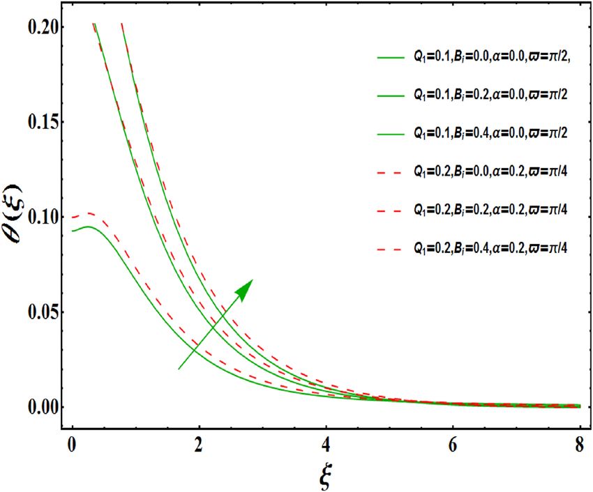
www.nature.com/scientificreports/

                                  Figure 5.  Variation of M1 on F ′ (ξ ) for both with and without inclanation.

                                  Figure 6.  Variation of We on F ′ (ξ ) for both with and without inclanation.

                                  to specific process times. Growing We causes a reduction in specific process time that consequence will lead a
                                  decline in velocity component and BL thickness. Further, we noticed that velocity field is remarkably higher in
                                  inclined MHD case than non-inclined MHD. The finding in Fig. 7 describes that velocity profile is declining
                                  functions of unsteadiness variable in BL for both scenarios of inclination parameter ̟ i.e., non-inclined MHD
                                  (̟ = π/2) and inclined MHD (̟ = π/3). This is owing to the belief that as unsteadiness factor S1 grows, the
                                  velocity of stretched surface also reduces that further causes the conversion of less amount of heat and mass
                                  from the plate to the fluid in the boundary layer region. Figure 8 is sketched to view the distribution of fluid
                                  velocity for several values of suction parameter (A > 0) for two separate scenarios of inclination parameter ̟
                                  i.e., non-inclined MHD (̟ = π/2) and inclined MHD (̟ = π/3). It can be noted that when the values of the
                                  suction parameter rises, the velocity field and associated boundary layer thickness are lessened for both cases.
                                  This is bases the fact that suction or blowing is the way of controlling the boundary layer. The suction method
                                  involves extracting decelerated liquid particles from the boundary layer until they are given the opportunity to
                                  cause separation. Moreover, we noticed that velocity field is higher in inclined MHD case than non-inclined
                                  MHD. Figure 9 demonstrates the velocity field F ′ (ξ ) for different values of injection (A < 0) for both scenarios
                                  of inclination parameter ̟ i.e., non-inclined MHD (̟ = π/2) and inclined MHD (̟ = π/3). This figure
                                  illustrates that velocity grow with an improvement in injection parameter for both cases. Furthermore, we noted
                                  that velocity field is declines in case of non-inclined MHD (̟ = π/2) than inclined MHD (̟ = π/3). The influ-
                                  ence of electric parameter E1 on fluid velocity field F ′ (ξ ) is showed in Fig. 10 for both scenarios of inclination
                                  parameter ̟ i.e., non-inclined MHD (̟ = π/2) and inclined MHD (̟ = π/4). We scrutinized that the related
                                  boundary layer grows at a slightly lower rate near the wall for greater values of electrical parameter E1, whereas

Scientific Reports |   (2021) 11:14509 |               https://doi.org/10.1038/s41598-021-93790-9                                                    9

                                                                                                                                                Vol.:(0123456789)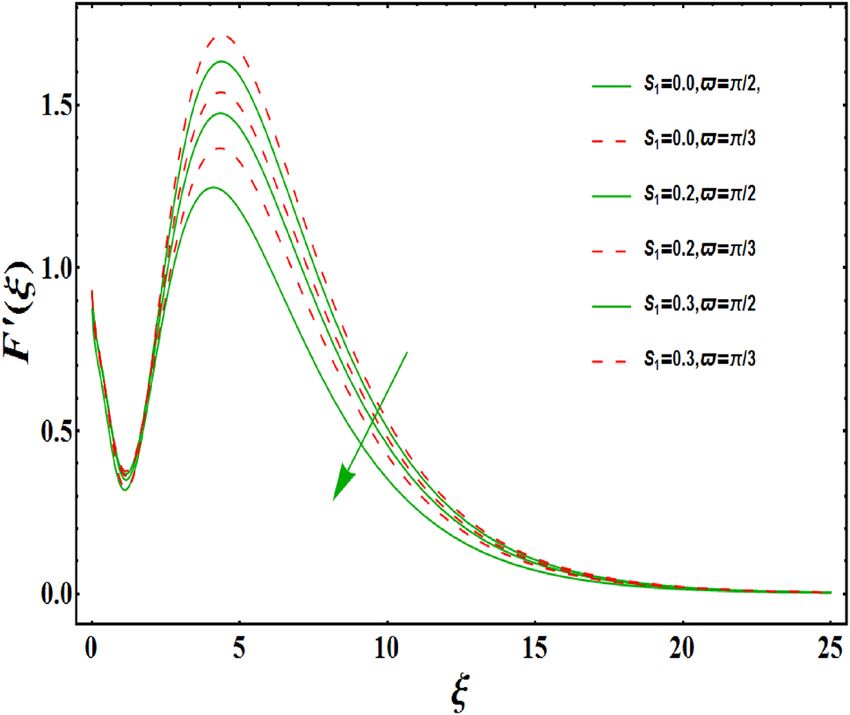
www.nature.com/scientificreports/

                                            Figure 7.  Variation of S1 on F ′ (ξ ) for both with and without inclanation.

                                            Figure 8.  Variation of A > 0 on F ′ (ξ ) for both with and without inclanation.

                                            it tends to increase more dramatically away from the stretching surface for both situations. This study indicates
                                            that moving the streamlines away from the extended boundary is the consequence of electrical parameters. It
                                            is due to the Lorentz force that causes reduction in the frictional resistance. In addition, we found that velocity
                                            field is significantly higher in case of inclined MHD than non-inclined MHD for electrical parameter E1. For
                                            several values of velocity slip parameter γ1 , the variability of velocity field is mapped in Fig. 11 for both case of
                                            inclination parameter ̟ i.e., non-inclined MHD (̟ = π/2) and inclined MHD (̟ = π/4). Figure 11 clearly
                                            demonstrates that velocity curves drop significantly as value of velocity slip number rises for both cases when
                                            ̟ = π/2 and ̟ = π/4 . This is owing to the belief that slip velocity grows as slip parameter rises and liquid
                                            velocity declines as the pulling of stretching wall can only be partially transmitted to the fluid under the slip
                                            condition. Figures 12 and 13 are plotted to observed the variability of temperature field θ(ξ ) for different values
                                            of the suction/injection parameter (A > 0, A < 0), respectively for both non-inclined MHD (̟ = π/2) and
                                            inclined MHD (̟ = π/4). From said figures, it can be noted that enhancement in suction parameter (A > 0)
                                            causes the reduction in temperature and associated boundary layer thickness whereas opposite behaviour is
                                            noted for the injection (A < 0) parameter when ̟ = π/2 and ̟ = π/4. Furthermore, in case of non-inclinied
                                            MHD, temperature field is remarkably higher. The finding in Fig. 14 indicates that the temperature profile θ(ξ )
                                            is enhanced by the rise in thermal radiation R1 for both scenarios of inclination parameter ̟ i.e., non-inclined
                                            MHD (̟ = π/2) and inclined MHD (̟ = π/4) and also for electric parameter when E1 = 0.1, 0.2. This is based
                                            on the fact that the increment in radiation parameter gives more heat to liquid which permitting the rise in tem-
                                            perature and thermal boundary layer thickness. Now, we elaborate the influence of electric parameter E1 on the

          Scientific Reports |   (2021) 11:14509 |               https://doi.org/10.1038/s41598-021-93790-9                                                    10

Vol:.(1234567890)
www.nature.com/scientificreports/
Figure 9. Variation of A < 0 on F ′ (ξ ) for both with and without inclanation.
Figure 10. Variation of E1 on F ′ (ξ ) for both with and without inclanation.
temperature field as it has also a strong physical significance on the fluid temperature. Figure 14 also demonstrates
that there is high temperature and associated boundary layer thickness for increment in electric parameter E1.
Additionally, it is found that for both radiation and electric parameters the temperature field upsurges for the
case of inclined MHD (̟ = π/4). Figure 15 show the variability of temperature field for several values of heat
source parameter Q1 , Biot number Bi and thermal slip parameter α for both scenarios of inclination parameter
̟ i.e., non-inclined MHD (̟ = π/2) and inclined MHD (̟ = π/4). It is noted that the temperature field rises
with an increament of the heat source. Also similar trend is happening for higher values of Biot and thermal slip
parameter α for both situations.
The values of SFC and NN for different values of related parameters are presented in Tables 3 and 4 for both
inclined and non-inclined MHD by taking ̟ = π/6, π/2 respectively. It can be observed that SFC reduces with
increment in Weissenberg number, unsteady number, velocity slip parameter, and suctions parameter (A > 0)
while the opposite pattern is observed for local electric parameter, magnetic number and injection variable
(A < 0) for both cases. It is examined that NN reduces with an increase in the magnetic parameter, Prandtl vari-
able, thermal slip number and heat absorption parameter (Q1 < 0), whereas it grows with an increase in electric
number, radiation number, Eckert parameter, Biot number and heat generation number (Q1 > 0) for both cases.
The outcomes attained from the numerical modeling and ANN model are in quite strong agreement with the
numerical outputs. The suggested ANN model is therefore effective for unsteady hydromagnetic Williamson
liquid flow along the radiative surface via heat absorption/generation and convective boundary condition, based
on results of the current study.
Scientific Reports | (2021) 11:14509 | https://doi.org/10.1038/s41598-021-93790-9 11
Vol.:(0123456789)www.nature.com/scientificreports/
Figure 11. Variation of γ1 on F ′ (ξ ) for both with and without inclanation.
Figure 12. Variation of A > 0 on θ (ξ ) for both with and without inclanation.
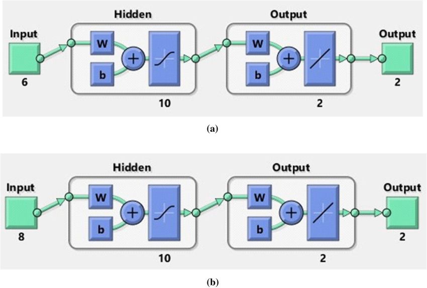
The training performances of both ANN models developed in Fig. 16 are shown. It is clear from the graphs
that the MSE values, which have high values at the beginning of the training process, decrease with the advancing
epochs. The ANN model, which has been developed to predict the Skin Friction Coefficients value, reached the
best point by reaching the lowest MSE value in the 4th epoch. The ANN model developed to predict the Nusselt
Number reached the lowest MSE value in the 7th epoch. This situation indicates that the training phase of ANN
models has been completed with high performance. Figure 17 shows the data obtained from the training phase of
ANN models. While there are target values on the x-axis of the graphs, there are ANN predictions on the y-axis.
When the location of the data points obtained from the data used in the training phase of both developed models
is examined, it is seen that they are located on the equality line drawn in blue. The R value for the ANN model
developed for the Skin Friction Coefficients prediction is 0.99928 and the R value for the ANN model developed
for the prediction of the Nusselt Number is calculated as 0.99999. These values show that the training phase of
both ANN models has been ideally completed. Figure 18 shows the performance of the validation stage of both
ANN models. When the graph is examined, it is seen that the data points obtained from the validation stage
are close to the equality line drawn in green. However, R values for the models have been calculated as 0.99015
and 0.96602, respectively. The data obtained confirm that the validation stage of both ANN models has been
completed with low error rates. In Fig. 19, the test stages of both ANN models is shown. It should be noted that
the data points obtained from the test stages in the graphics are located close to the equality line drawn in red. R
values of ANN models have been obtained as 0.98102 and 0.95998, respectively. These results clearly show that the
test stages of ANN models have been completed with high accuracy. Figure 20 shows the MSE values obtained for
Scientific Reports | (2021) 11:14509 | https://doi.org/10.1038/s41598-021-93790-9 12
Vol:.(1234567890)www.nature.com/scientificreports/
Figure 13. Variation of A < 0 on θ (ξ ) for both with and without inclanation.
Figure 14. Variation of R1 on θ(ξ ) for both with and without inclanation.
Figure 15. Variation of Bi on θ(ξ ) for both with and without inclanation.
Scientific Reports | (2021) 11:14509 | https://doi.org/10.1038/s41598-021-93790-9 13
Vol.:(0123456789)www.nature.com/scientificreports/
Figure 16. Performance of the ANN (a) Skin Friction Coefficients (b) Nusselt Number.
Figure 17. Training data (a) Skin Friction Coefficients (b) Nusselt Number.
each data point of the ANN models developed. While there are data points on the x-axis of the charts, there are
MSE values on the y-axis. It should be noted that the values obtained by the calculated MSE values are quite low.
The low values reached by the MSE values are another indication that both ANN models are ideally developed.
In analyzing the performance of ANNs, it is important to analyze the error rates between predicted values and
target values. For this purpose, error rates have been calculated and analyzed for each data point. In Fig. 21 the
error rates of both ANN models are shown for each data point. When the graphics are examined, it is seen that
the error rates of both models are low. When the error rates are evaluated, it is seen that the developed ANN
models can predict Skin Friction Coefficients and Nusselt Numbers with acceptable error rates. Figure 22 shows
the comparison of the prediction data obtained from both ANN models with the numerical data which are the
target values. While there are target data on the x-axes of the graphs, there are ANN predictions on the x-axes.
Scientific Reports | (2021) 11:14509 | https://doi.org/10.1038/s41598-021-93790-9 14
Vol:.(1234567890)www.nature.com/scientificreports/
Figure 18. Validation data (a) Skin Friction Coefficients (b) Nusselt Number.
Figure 19. Test data (a)Skin Friction Coefficients (b) Nusselt Number.
When the graphs are examined, it is seen that the data points obtained from both ANN models are located on
the equality line. This state of the data points confirms that both ANN models are developed to be able to predict
with high accuracy. Numerical values of performance parameters of both ANN models are given in Table 2.
Final remarks
In current study we successfully utilized the ANN approach for prediction of electro-hydrodynamic BLSF of Wil-
liamson fluid towards a permeable stretched surface under heat generation/absorption and convective boundary
condition. The data attained from the training, validation and testing stages of the proposed ANN model have
been analyzed with numerical techniques and proved to have excellent prediction accuracy. The presented ANN
model is reliable, effective and time saving as it requires less effort and provides quick results than numerical
techniques. Furthermore, it is inferred that the developed ANN model may be regarded as an appropriate and
Scientific Reports | (2021) 11:14509 | https://doi.org/10.1038/s41598-021-93790-9 15
Vol.:(0123456789)www.nature.com/scientificreports/
0,12 0,15
Skin Friction Coefficients Nusselt Number
0,10
0,10
0,08
0,06
0,05
0,04
MSE
MSE
0,02 0,00
0,00
-0,05
-0,02
-0,04
-0,10
/2
-0,06 /2
/6
/6
-0,08 -0,15
0 5 10 15 20 25 30 0 5 10 15 20 25 30 35
Data Number Data Number
Figure 20. MSE values (a) Skin Friction Coefficients (b) Nusselt Number.
10 10
Skin Friction Coefficients Nusselt Number
5 5
Error Rate (%)
Error Rate (%)
0 0
-5 -5
/2 /2
/6 /6
-10 -10
0 5 10 15 20 25 30 0 10 20 30
Data Number Data Number
Figure 21. Error rates (a) Skin Friction Coefficients (b) Nusselt Number.
effective approach for solving the heat transfer aspects with Newtonian/non-Newtonian fluid flow challenges.
The main key points of this study as follows:
• The velocity profile is lessened for increment in both magnetic and Wessinberg numbers.
• Temperature field rises with an increament of the heat source while similar trend is noted for higher values
of Biot and thermal slip parameter.
• Skin friction coefficient reduces with increasing values of Weissenberg parameter, unsteady parameter for
both inclined and non-inclined MHD cases.
• For the ANN model developed to predict the Skin Friction Coefficients values, the MSE value is 1.93 × 10⁻³,
the R value is 0.99540 and the average error rate is 0.57%.
Scientific Reports | (2021) 11:14509 | https://doi.org/10.1038/s41598-021-93790-9 16
Vol:.(1234567890)www.nature.com/scientificreports/
0,7
1,2
Skin Friction Coefficients Nusselt Number
1,0 0,6
0,8
ANN Prediction
ANN Prediction
0,5
0,6
0,4
0,4
0,3
0,2 Data Point ( /2) Data Point ( /2)
Data Point ( /6) 0,2 Data Point ( /6)
0,2 0,4 0,6 0,8 1,0 1,2 0,2 0,3 0,4 0,5 0,6 0,7
Numerical Values Numerical Values
Figure 22. Numerical values vs ANN Prediction (a) Skin Friction Coefficients (b) Nusselt Number.
xk Bk
0.137793 0.308441116
0.729455 0.401119929
1.80834 0.218068288
3.40143 0.062087456
5.5525 0.009501517
8.33015 0.000753008
11.8438 0.000028259
16.2793 4.24931 × 10⁻⁷
21.9966 1.83956 × 10⁻⁹
29.9207 9.91183 × 10⁻¹³
Table 1. Arguments xk and corresponding coefficients Ak.
Skin Friction Coefficients Nusselt Number
MSE R MoD MSE R MoD
Train 1.27 × 10−04 0.99928 0.27 2.95 × 10−07 0.99999 0.09
Validation 2.61 × 10−03 0.99015 1.82 9.85 × 10−04 0.96602 −1.06
Test 3.07 × 10−03 0.98102 0.86 9.22 × 10−03 0.95998 0.02
All 1.93 × 10−03 0.99540 0.57 3.40 × 10−03 0.93413 −0.10
Table 2. Numerical values of performance parameters of ANN models.
• For the ANN model developed to predict the Nusselt Number, the MSE value has been calculated as
3.40 × 10⁻³, the R value as 0.93413 and the average error rate as −0.10%.
• These results showed that the developed ANN models have been developed in such a way that they can
calculate Skin Friction Coefficients and Nusselt Number values with very low error rates and high accuracy.
• The results obtained from the study revealed that ANNs are one of the ideal tools that can be used to predict
the Skin Friction Coefficients and Nusselt Number values.
Scientific Reports | (2021) 11:14509 | https://doi.org/10.1038/s41598-021-93790-9 17
Vol.:(0123456789)www.nature.com/scientificreports/
1
−Rex̂2 C̃F
GWRM ANN Prediction
We A S1 M1 E1 γ1 ̟ = π/2 ̟ = π/6 ̟ = π/2 ̟ = π/6
0.0 0.2 0.2 0.2 0.2 0.2 1.121120 1.088250 1.112467812 1.083272461
0.1 1.043753 1.024818 1.048470245 1.032320827
0.2 0.947400 0.934794 0.929619336 0.920865489
0.3 0.813207 0.808549 0.796758184 0.79651443
0.4 0.423486 0.383934 0.415797181 0.378361069
0.5 0.197690 0.201845 0.197602484 0.200345792
0.6 0.118298 0.120898 0.114536525 0.11686413
0.4 −0.3 0.2 0.2 0.3 0.2 0.579218 0.624945 0.579849492 0.622467226
−0.1 0.534282 0.612793 0.525415549 0.613342799
0.0 0.528116 0.593290 0.541500147 0.59608308
0.1 0.526469 0.553815 0.525230251 0.54687993
0.3 0.255066 0.254418 0.264369837 0.264359103
0.4 0.2 0.0 0.2 0.3 0.2 0.574345 0.567663 0.559570812 0.570079188
0.2 0.461392 0.426647 0.462441292 0.430436492
0.4 0.265973 0.266549 0.263805884 0.274831381
0.6 0.226133 0.226746 0.222296971 0.221554163
0.4 0.2 0.2 0.0 0.3 0.2 0.338589 0.338589 0.328381059 0.327822824
0.1 0.426647 0.346803 0.427074483 0.355467855
0.2 0.461392 0.426647 0.470441292 0.430436492
0.3 0.468562 0.445113 0.461320839 0.439161544
0.4 0.2 0.2 0.3 0.0 0.2 0.255378 0.291616 0.256710308 0.295370046
0.2 0.367085 0.422143 0.365989456 0.427634432
0.4 0.466563 0.468116 0.454175184 0.450696484
0.6 0.468732 0.477804 0.455011903 0.479954302
0.2 0.2 0.2 0.2 0.2 0.0 1.163880 1.139770 1.150888953 1.126683758
0.1 1.052630 1.036790 1.044065726 1.034083472
0.2 0.947401 0.934794 0.929619336 0.920865489
0.3 0.864947 0.845393 0.850830626 0.836475263
1
Table 3. Numerical values of skin friction coefficients Rex̂2 C̃F for different values of physical parameters.
Received: 16 March 2021; Accepted: 24 June 2021
References
1. Abegunrin, O. A. & Animasaun, I. L. Motion of Williamson fluid over an upper horizontal surface of a paraboloid of revolution
due to partial slip and buoyancy: boundary layer analysis. Defect Diffusion Forum. 378, 16–27 (2017).
2. Abegunrin, O. A., Okhuevbie, S. O. & Animasaun, I. L. Comparison between the flow of two non-Newtonian fluids over an upper
horizontal surface of paraboloid of revolution: boundary layer analysis. Alex. Eng. J. 55(3), 1915–1929 (2016).
3. Ghulam, R. et al. Entropy generation and consequences of binary chemical reaction on MHD Darcy-Forchheimer Williamson
nanofluid flow over non-linearly stretching surface. Entropy 22(1), 18 (2020).
4. Shafiq, A., Rashidi, M. M., Hammouch, Z. & Khan, I. Analytical investigation of stagnation point flow of Williamson liquid with
melting phenomenon. Phys. Scr. 94(3), 035204 (2019).
5. Shafiq, A. & Sindhu, T. N. Statistical study of hydromagnetic boundary layer flow of Williamson fluid regarding a radiative surface.
Results Phys. 7, 3059–3067 (2017).
6. Khan, M., Malik, M. Y., Salahuddin, T. & Hussian, A. Heat and mass transfer of Williamson nanofluid flow yield by an inclined
Lorentz force over a nonlinear stretching sheet. Results Phys. 8, 862–868 (2018).
7. Khan, N. A., Khan, S. & Riaz, F. Boundary layer flow of Williamson fluid with chemically reactive species using scaling transforma-
tion and homotropy analysis method. Math. Sci. Lett. 3(3), 199–205 (2014).
8. Hashim, A., Hamid, M., Khan, M. & Khan, U. Thermal radiation effects on Williamson fluid flow due to an expanding/contracting
cylinder with nanomaterials: dual solutions. Phys. Lett. A 382(30), 1982–1991 (2018).
9. Khan, M. & Hamid, A. Influence of non-linear thermal radiation on 2D unsteady flow of a Williamson fluid with heat source/sink.
Results Phys. 7, 3968–3975. https://doi.org/10.1016/j.rinp.2017.10.014 (2017).
10. Khan, Md. S., Karim, I., Islam, Md. S. & Wahiduzzaman, O. MHD boundary layer radiative, heat generating and chemical reacting
flow past a wedge moving in a nanofluid. Nano Converg. 5, 1–20. https://doi.org/10.1186/s40580-014-0020-8 (2014).
11. Hayat, T., Shafiq, A. & Alsaedi, A. Hydromagnetic boundary layer flow of Williamson fluid in the presence of thermal radiation
and Ohmic dissipation. Alex. Eng. J. 55(3), 2229–2240 (2016).
12. Hayat, T., Shafiq, A. & Alsaedi, A. Effect of Joule heating and thermal radiation in flow of third grade fluid over radiative surface.
PLoS ONE 9(1), e83153 (2014).
13. Hayat, T., Shaheen, U., Shafiq, A., Alsaedi, A. & Asghar, S. Marangoni mixed convection flow with Joule heating and nonlinear
radiation. AIP Adv. 5(7), 077140 (2015).
Scientific Reports | (2021) 11:14509 | https://doi.org/10.1038/s41598-021-93790-9 18
Vol:.(1234567890)www.nature.com/scientificreports/
−1/2
−Rex Nux̂
GWRM ANN Prediction
M1 E1 R1 Pr Ec Q1 Bi α ̟ = π/2 ̟ = π/6 ̟ = π/2 ̟ = π/6
0.0 0.3 0.3 1 0.5 0.5 0.2 0.2 0.417812 0.417812 0.417622065 0.417011494
0.2 0.417615 0.417798 0.416708272 0.417312171
0.4 0.413635 0.417615 0.413437193 0.416625828
0.6 0.409676 0.416479 0.409060414 0.415986525
0.2 0.0 0.3 1 0.5 0.5 0.2 0.2 0.401078 0.414855 0.401080763 0.414687452
0.1 0.409927 0.415234 0.409457697 0.415549836
0.2 0.411936 0.416209 0.412264956 0.415243645
0.3 0.417615 0.417798 0.416708272 0.417312171
0.2 0.3 0.0 1 0.5 0.5 0.2 0.2 0.268871 0.268210 0.268799609 0.268001409
0.2 0.365731 0.365844 0.364971655 0.365299625
0.4 0.471390 0.471922 0.47056126 0.471221267
0.6 0.583913 0.585162 0.578643641 0.580752337
0.2 0.3 0.3 0.8 0.5 0.5 0.2 0.2 0.393609 0.394120 0.393078442 0.393476331
0.9 0.378502 0.378705 0.391306506 0.387579291
1.0 0.365730 0.365836 0.356708272 0.357312171
1.1 0.355096 0.354673 0.35485935 0.354320921
0.2 0.3 0.3 1.0 0.0 0.5 0.2 0.2 0.254696 0.256038 0.256716643 0.254569521
0.3 0.352399 0.353061 0.352157083 0.352463088
0.6 0.450119 0.450186 0.449328272 0.449794601
0.9 0.547505 0.547101 0.546883625 0.546264445
0.2 0.3 0.3 1.0 0.5 −0.4 0.2 0.2 0.255003 0.254178 0.249302396 0.248048876
−0.2 0.273659 0.272779 0.281062975 0.282322934
0.0 0.297440 0.296601 0.297826133 0.296945579
0.2 0.329769 0.328813 0.330039994 0.329025368
0.4 0.378853 0.378246 0.39093441 0.391221193
0.2 0.3 0.3 1.0 0.5 0.5 0.0 0.3 0.199100 0.197921 0.20215141 0.204587407
0.2 0.403670 0.403598 0.402736781 0.403118255
0.4 0.548724 0.549310 0.548508547 0.548963569
0.6 0.655744 0.656985 0.662586879 0.638124434
0.2 0.3 0.3 1.0 0.5 0.5 0.3 0.0 0.542491 0.542391 0.542129796 0.541764069
0.1 0.51954 0.520165 0.519009327 0.519677028
0.2 0.499513 0.500135 0.499251651 0.499576203
0.3 0.481828 0.482317 0.481695049 0.481651657
−1/2
Table 4. Numerical values of Nusselt number Rex Nux for different values of physical parameters A = 0.3,
S1 = 0.0.2, We = 0.4, γ1 = 0.2.
14. Shafiq, A., Khan, I., Rasool, G., Seikh, A. H. & Sherif, El-Sayed M. Significance of double stratification in stagnation point flow of
third-grade fluid towards a radiative stretching cylinder. Mathematics 7(11), 1103 (2019).
15. Shafiq, A., Hammouch, Z. & Oztop, Hakan F. Radiative MHD flow of third-grade fluid towards a stretched cylinder. In International
Conference on Computational Mathematics and Engineering Sciences 166–185 (Springer, Cham, 2019).
16. Hayat, T., Jabeen, S., Shafiq, A. & Alsaedi, A. Radiative squeezing flow of second grade fluid with convective boundary conditions.
PLoS ONE 11(4), e0152555 (2016).
17. Shafiq, A., Sindhu, T. N. & Hammouch, Z. Characteristics of homogeneous heterogeneous reaction on flow of Walters’ B liquid
under the statistical paradigm. In International workshop of Mathematical Modelling, Applied Analysis and Computation 295–311
(Springer, Singapore, 2018).
18. Rasool, G. et al. Entropy generation and consequences of MHD in Darcy-Forchheimer nanofluid flow bounded by non-linearly
stretching surface. Symmetry 12(4), 652 (2020).
19. Mabood, F., Tlili, I. & Shafiq, A. Features of inclined magnetohydrodynamics on a second-grade fluid impinging on vertical
stretching cylinder with suction and Newtonian heating. Mathematical Methods in the Applied Sciences (2020).
20. Shafiq, A. & Khalique, Chaudry Masood. Lie group analysis of upper convected Maxwell fluid flow along stretching surface. Alex.
Eng. J. 59(4), 2533–2541 (2020).
21. Shafiq, A., Sindhu, T. N. & Al-Mdallal, Q. M. A sensitivity study on carbon nanotubes significance in Darcy–Forchheimer flow
towards a rotating disk by response surface methodology. Sci. Rep. 11(1), 1–26 (2021).
22. Shafiq, A., Mebarek-Oudina, F., Sindhu, T. N. & Abidi, A. A study of dual stratification on stagnation point Walters’ B nanofluid
flow via radiative Riga plate: a statistical approach. Eur. Phys. J. Plus 136(4), 1–24 (2021).
23. Shafiq, A., Sindhu, T. N. & Khalique, C. M. Numerical investigation and sensitivity analysis on bioconvective tangent hyperbolic
nanofluid flow towards stretching surface by response surface methodology. Alex. Eng. J. 59(6), 4533–4548 (2020).
Scientific Reports | (2021) 11:14509 | https://doi.org/10.1038/s41598-021-93790-9 19
Vol.:(0123456789)www.nature.com/scientificreports/
24. Shafiq, A., Hammouch, Z., Sindhu, T. N. & Baleanu, D. Statistical approach of mixed convective flow of third-grade fluid towards an
exponentially stretching surface with convective boundary condition. Special Functions and Analysis of Differential Equations2020,
307.
25. Reza-E-Rabbi, S., Arifuzzaman, S. M., Sarkar, T., Khan, M. S. & Ahmmed, S. F. Explicit finite difference analysis of an unsteady
MHD flow of a chemically reacting Casson fluid past a stretching sheet with Brownian motion and thermophoresis effects. J. King
Saud Univ.-Sci. 32(1), 690–701 (2020).
26. Arifuzzaman, S. M., Khan, M. S., Mehedi, M. F. U., Rana, B. M. J. & Ahmmed, S. F. Chemically reactive and naturally convective
high speed MHD fluid flow through an oscillatory vertical porous plate with heat and radiation absorption effect. Eng. Sci. Technol.
Int. J. 21(2), 215–228 (2018).
27. Arifuzzaman, S. M. et al. Hydrodynamic stability and heat and mass transfer flow analysis of MHD radiative fourth-grade fluid
through porous plate with chemical reaction. J. King Saud Univ.-Sci. 31(4), 1388–1398 (2019).
28. Rasoola, G. & Shafiq, A. Darcy-Forchheimer relation in Magnetohydrodynamic Jeffrey nanofluid flow over stretching surface.
Discrete & Continuous Dynamical Systems-S (2018).
29. Das, K. Slip effects on MHD mixed convection stagnation point flow of a micro-polar fluid towards a shrinking vertical sheet.
Comput. Math. Appl. 63, 255–267 (2012).
30. Shafiq, A., Rasool, G. & Khalique, C. M. Significance of thermal slip and convective boundary conditions in three dimensional
rotating Darcy-Forchheimer nanofluid flow. Symmetry 12(5), 741 (2020).
31. Mabood, F., Shafiq, A., Hayat, T. & Abelman, S. Radiation effects on stagnation point flow with melting heat transfer and second
order slip. Results Phys. 7, 31–42 (2017).
32. Reddy, P. B. A., Suneetha, S. & Reddy, N. B. Numerical study of magnetohydrodynamics (MHD) boundary layer slip flow of a
Maxwell nanofluid over an exponentially stretching surface with convective boundary condition. Propuls. Power Res. 6(4), 259–268
(2017).
33. Khan, M. Hashim, Effects of multiple slip on flow of magnetoCarreau fluid along wedge with chemically reactive species. Neural
Comput. Appl. 1–13 (2016).
34. Razaq, A. O. & Aregbesola, Y. K. S. Weighted residual method in a semi infinite domain using un-partitionedmethod. Int. J. Appl.
Math. 25, 25–31 (2012).
35. Scheid, F. Numerical Analysis, Schaum’s Outline Series 135–139 (McGraw-Hill Book Company, 1964).
36. Li, L. et al. Stability, thermal performance and artificial neural network modelingof viscosity and thermal conductivity of Al2O3-
ethylene glycol nanofluids. Powder Technol. 363, 360–368 (2020).
37. Çolak, A. B. A novel comparative analysis between the experimental and numeric methods on viscosity of zirconium oxide nano-
fluid: Developing optimal artificial neural network and new mathematical model. Powder Technol. 381, 338–351 (2021).
38. Ariana, M. A., Vaferi, B. & Karimi, G. Prediction of thermal conductivity of alumina water-based nanofluids byartificial neural
networks. Powder Technol. 278, 1–10 (2015).
39. Peng, Y. et al. Analysis of the effect of roughness and concentration of Fe3O4/waternanofluid on the boiling heat transfer using
the artificial neural network: An experimental and numerical study. Int. J. Therm. Sci. 163, 106863 (2021).
40. Verma, J. & Lal, S. Nanoparticles for hyperthermic therapy: Synthesisstrategies and applications in glioblastoma. Int. J. Nanomed.
9, 2863–2877 (2014).
41. Benos, LTh., Spyrou, L. A. & Sarris, I. E. Development of a new theoretical model forblood-CNTs effective thermal conductivity
pertaining to hyperthermia therapy ofglioblastoma multiform. Comput. Meth. Prog. Biol. 172, 79–85 (2019).
42. Akhgar, A. et al. Developing dissimilar artificial neural networks(ANNs) to prediction the thermal conductivity of MWCNT-TiO2/
water-ethylene glycolhybrid nanofluid. Powder Technol. 355, 602–610 (2019).
43. Çolak, A. B., Akçaözoğlu, K., Akçaözo ğlu, S. & Beller, G. Artificial intelligence approach in predicting the effect of elevated
temperature on the mechanical properties of PET aggregate mortars: An experimental study. Arabian Journal for Science and
Engineering. https://doi.org/10.1007/s13369-020-05280-1 (2021).
44. Çolak, A. B. Developing optimal artificial neural network (ANN) to predict the specific heat of water based yttrium oxide (Y2O3)
nanofluid according to the experimental data and proposing new correlation. Heat Transfer Res. 51(17), 1565–1586 (2020).
45. Canakci, A., Varol, T. & Ozsahin, S. Analysis of the effect of a new process control agenttechnique on the mechanical milling
process using a neural network model:measurement and modeling. Measurement 46, 1818–1827 (2013).
46. Vaferi, B., Samimi, F., Pakgohar, E. & Mowla, D. Artificial neural network approach forprediction of thermal behavior of nanofluids
flowing through circular tubes. PowderTechnol. 267, 1–10 (2014).
47. Çolak, A. B. An experimental study on the comparative analysis of the effect of the number of data on the error rates of artificial
neural networks. Int. J. Energy Res. 45(1), 478–500 (2021).
48. Ali, A. et al. Dynamic viscosity of Titania nanotubes dispersions in ethylene glycol/water-based nanofluids: Experimental evaluation
and predictions from empirical correlation and artificial neural network. Int. Commun. Heat Mass Transfer 118, 104882 (2020).
49. Bonakdari, H. & Zaji, A. H. Open channel junction velocity prediction by using a hybridself-neuron adjustable artificial neural
network. Flow Meas. Instrum. 49, 46–51 (2016).
50. He, W. et al. Using of Artificial Neural Networks (ANNs) to predict the thermal conductivity of Zinc Oxide-Silver (50%-50%)/
Water hybrid Newtonian nanofluid. Int. Commun. Heat Mass Transfer 116, 104645 (2020).
51. Vafaei, M. et al. Evaluation of thermal conductivity of MgO-MWCNTs/EG hybrid nanofluids based on experimental data by
selecting optimal artificialneural networks. Physica E 85, 90–96 (2017).
52. Çolak, A. B. Experimental study for thermal conductivity of water-based zirconium oxide nanofluid: Developing optimal artificial
neural network and proposing new correlation. Int. J. Energy Res. 45(2), 2912–2930 (2020).
Author contributions
All authors have equal contribution.
Competing intrests
The authors declare no competing interests.
Additional information
Correspondence and requests for materials should be addressed to Q.M.A.-M.
Reprints and permissions information is available at www.nature.com/reprints.
Publisher’s note Springer Nature remains neutral with regard to jurisdictional claims in published maps and
institutional affiliations.
Scientific Reports | (2021) 11:14509 | https://doi.org/10.1038/s41598-021-93790-9 20
Vol:.(1234567890)You can also read