Equatorial Platform Based on Planer Linkage
←
→
Page content transcription
If your browser does not render page correctly, please read the page content below
Equatorial Platform Based on Planer Linkage
                                                                            Daniel J Matthews
arXiv:2106.15694v1 [astro-ph.IM] 29 Jun 2021

                                                                              matth036@umn.edu

                                                                                July 1, 2021

                                               Area of Technology
                                               Visual and photograpic astronomy. Telescope mounts. Solar tracking for energy
                                               collection.

                                               What is an Equatorial Platform?
                                               An equatorial platform is a mechanism upon which a telescope on a non-tracking
                                               mount may be placed and the motion of the mechanism will result in tracking.
                                               Here tracking means the object under observation remains centered in the field
                                               of view of the telescope. An equatorial platform can only track for a limited
                                               time period before it must be reset.
                                                   Appendix D of reference [2] discusses equatorial platforms including some
                                               history.

                                               Preliminary Discussion of the Roberts Linkage
                                               A great variety of planar linkages are known to mechanical engineers. Some of
                                               these linkages feature a tracer point whose trajectory describes an approximate
                                               straight line. The Roberts linkage is one such mechanism. Reference [1] at-
                                               tributes the linkage to Richard Roberts of Manchester and dates the invention
                                               as prior to 1841.
                                                   Figures 1a and 1b illustrate an example of a Roberts linkage. Two fixed
                                               pivots are attached to two equal length struts. The other end of these struts are
                                               attached to two equal angle corners of an isoceles triangle with the short side
                                               acting as a connecting link. The equal long sides of the triangle have the same
                                               length as the two struts. The short side of the triangle has length equal to half
                                               the distance between the two fixed pivots. In motion the vertex of the triangle
                                               acts as a tracing point whose trajectory deviates very little from a straight line.

                                                                                       1
Figure 1: Roberts Linkage
(a) Centered (b) Inclined 7.6◦
Application of the Roberts Linkage to an Equato-
rial Tracking Device
Position the plane of motion of a Roberts linkage to be same plane as the celestial
equator. The normal to this plane will be directed toward the celestial pole. In
the northern hemisphere this is near Polaris. This positioning is effectively polar
alignment.
We shall call the center piece in motion the lamina. With out violating the
above positioning reqirement we can arrange for the approximate straight line
motion of the tracer point on the lamina to be horizontal.
The constrained motion of the lamina comprises both rotation and transla-
tion. If pushed at a properly selected rate, the rotation can nullify the diurnal
rotation of the earth. This is the purpose of the present invention. While the
translational motion brings no benefit it is harmless when viewing objects at
astronomical distances.
Upon the lamina a shelf or attachment can be installed to hold a payload
telescope with altazimuth mount.
It can be further arranged that the center of gravity of (lamina + shelf +
payload) lies at a point in space which, perpendicular projected into the plane
of the lamina, lies on the tracer point.
The celestial tracking motion will result in very little vertical movement of
the center of gravity of the since the motion of the tracer point differs little from
a horizontal line.
Because there is little vertical movement of the center of gravity, the gravi-
tational potential energy is nearly constant as the motion proceeds.
Because the gravitational potential energy is nearly constant, the force needed
to maintain the motion will be small.
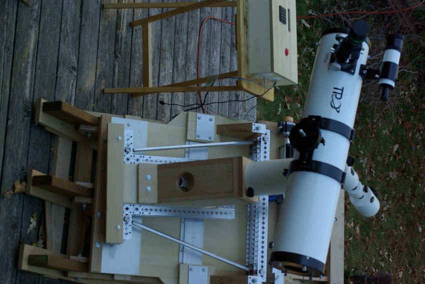
2Description of Existing Prototype
0.1 Mechanical
See Figure 2. A wooden frame provides a plane parallel to the celestial equator
at the observing site latitude 45◦ N.
The fixed upper pivots are 21 inches apart and the connecting lower link
has distance between pivots 10.5 inches apart. The east and west side links are
22.3125 inches long. The moving part is supported by PTFE (aka Teflon) sliders
below the lower pivots. Another slider is located on the center of the lamina
12.75 inches above the lower pivots. The surface under the sliders is Fiberglass
Reinforced Plastic (FRP).
A wheel on the moving lamina is centered and projects above the line of the
upper fixed pivots. The height of the wheel axle above the lower two moving
pivots is 25.25 inches. This wheel is an inline skate wheel. A linear actuator
carries a plate that pushes this wheel.
A wooden square pillar stands on the lamina and attaches to a comercially
available metal round pillar (Vixen part 25167). On top of the round pillar
an altazimuth mount carrying a telescope can be attached. Care is taken with
counter weights to make sure the center of gravity of the altazimuth mount is
comparativly stationary as the telescope is moved for pointing.
0.2 Electro-Mechanical
A Nucleo-144 STM32F767 evaluation board is the microcontroller for the project.
A 4x4 matrix keypad and 4x20 character OLED display provide input and out-
put. Six AA batteries power the Nucleo board independently of the 24V power
supply for the stepper driver. Opto-isolators both protect the board and provide
voltage step up from 3.3V to 5V for output signals to the stepper driver.
The stepper motor has 400 steps per revolution and the stepper driver is set
to run with 16 microsteps. The lead screw in the linear actuator has a pitch of
8 mm. When tracking the the microcontroller sends pulses to the stepper driver
at a freqency indicated the right hand axis of Figure 6.
0.3 Lessons Learned
The full planned range of tilt of was 7.5◦ east or west allowing for one hour
of tracking. This was not possible because beyond a certain point the center
of gravity shifted enough that the moving part of the apparatus began to tip
over. In practice 3 inches of east or west movement of the push wheel seemed
safe. This allows for about 30 minutes of tracking. Note that we can space the
lower sliders further apart without changing the length of the connecting link.
It is not necessary that these sliders be directly under the link. This increased
spacing will increase the range of stable motion.
3Figure 2: 6” F/6 Newtonian on the Platform
4Initially the PTFE sliders moved on a surface of aluminum. A vibration was
visible through the eyepiece which is likely due to slip stick friction. Switching
to an FRP surface greatly reduced this. Further plans are to polish the FRP
with automobile wax. In the next prototype the lower sliders may be replaced
with wheels.
5Appendices
A Kinematical Design
Kinematical design is also called kinematic design or geometric design. A well
illustrated introduction to kinematical design is reference [5] pp.585-590. The
guiding principle is to have no more positioning constraints on a collection of
rigid bodies than are required to fix its configuration. This involves counting
degrees of freedom of the bodies being positioned.
The Roberts linkage as employed in this invention is well suited for kine-
matical design. The lamina, or any rigid body, considered as an object in three
dimesional space has six degrees of freedom. To fix its position in space six
constraints are required.
Three contact points against a plane ensure that any motion of the lamina
is indeed planar. In the existing prototype these contact points are low friction
sliders and the plane is parallel the celestial equator on a solidly constructed
frame.
The east and west side links provide two more constraints. This leaves one
degree of freedom which is the tilting motion of the lamina. The final degree of
freedom can be fixed by contact with an actuator.
B Solution of Configuration
This solution is a variation of the trigonometric construction shown in refer-
ence [3] p.20. Refer to Figure 3. E and W are fixed pivots. D and V are
moving pivots whose configuration is constrained by east link ED, west link
W V , and connecting link DV . Point Q is constructed at any distance from D
such that DQ is parallel to EW . Angle γ = 6 V DQ is the input describing the
tilt of the connecting link relative to EW . In the present invention we will want
γ to change at a constant rate equivilent to one revolution per sidereal day.
Given γ we wish to determine α = 6 W ED and β = 6 EW V . Define fixed
lengths:
f = ||EW ||
c = ||DV ||
e = ||ED||
w = ||W V || .
Construct auxillary point A such that AEDV is a parallelogram with EA k DV
and ED k AV . Note that 6 AEW = 6 V DQ = γ. Consider segment AW (not
drawn),
x = f − c · cos(γ)
y = c · sin(γ)
6Figure 3: Four Bar Linkage (Some say Three Bar)
α β
γ
are the components of AW parallel and perpendicular to EW .
p
d = x2 + y 2
is the length of AW and y
δ = arctan
x
is 6 AW E. Most computer languages allow the evalution of δ as atan2(y,x).
Applying the law of cosines to 4AW V yields
e2 = w2 + d2 − 2dw cos(β + δ)
or
w2 + d2 − e2
β = −δ + arccos .
2wd
7A similar argument can show that
e2 + d2 − w2
α = δ + arccos
2ed
with the same definitions of d and δ. The other angles in quadrangle EDV W
are:
6 EDV = 180◦ − α − γ
6 DV W = 180◦ − β + γ.
Note that the sum of all four angles, (α + β + 6 EDV + 6 DV W ), is 360◦ as
expected.
C Centro: The Center of Rotation
As discussed, in motion the lamina undergoes both translation and rotation.
One may ask, about what center does this rotation take place? A simple con-
struction locates this center which some textbooks call the centro. See e.g.
reference [4] p.217.
Refer again to Figure 3. If we extend the line segment ED representing the
east link and likewise extend line segment W V representing the west link these
lines will, if not parallel, intersect at some point. This point of intersection is
the centro. This construction is shown in Figure 4.
Suppose the triangular lamina is pushed by a horizontal actuator near the
vertex of the triangle. The lever arm about which rotation occurs is the dis-
placement from the centro to the contact point of the actuator on the lamina.
The length of this lever arm is approximately twice the altitude of the triangle.
The comparative lever arm length of a conventional equatorial mount is the
pitch radius of the Right Ascension worm wheel. The linkage based platform
can have a lever arm length greater by a factor of ten. This results in greater
precision which is a major advantage of the present invention.
D Dealing with Nonlinearity
D.1 One Way
For the existing prototype the parameters f , c, e, and w are:
f = 21.0 in
c = 10.5 in
e = 22.3125 in
w = 22.3125 in
Additionally we need two parameters specifying the position of the wheel on the
lamina. To do this we need to be specific about coordinate systems used.
8Figure 4: The intersection of the red lines is the centro
9On the stationary frame we choose a coordinate system with origin centered
on the midpoint of the line of the fixed pivots with x coordinate increasing to
the west and y coordinate increasing upwards. In this system points D and V
in figure 3 have negative y coordinate.
On the moving lamina we choose a coordinate system with origin on the
midpoint of the line of the moving pivots with x coordinate increasing to the
west and y coordinate increasing upwards.
The coordinates of the wheel axle in the moving lamina frame are:
x = 0.0 in
y = 25.25 in
The wheel so located projects above the line of the fixed pivots. The motion
of this wheel is primarily horizontal and the small vertical movement is not
perceptable. A linear actuator pushes this wheel. The linear actuator is driven
by a lead screw rotated by a stepper motor. The calculation of Appendix B
determines the coordinates of the wheel. Figure 5 shows that the tilt γ is nearly
a linear function of the x coordinate of the wheel.
We can calculate the derivatives of the push point coordinates by treating
the motion of the lamina as a small rotation about the centro. The derivative
dγ is plotted in Figure 6. This derivative is directly proportional to the rate
dx
at which the wheel must be pushed to achieve a desired constant value of dγ dt .
This in turn is directly proportional to the frequency at which pulses must be
delivered to the stepper driver. For the existing prototype this frequency is
indicated on the right hand axis of Figure 6.
So, one way of dealing with non-linearity is to keep track of the x coordinate
and send pulses to the stepper driver at a calculatable frequency dependent on
x.
D.2 Another Way
The existing apparatus uses a different way of handling non-linearity. In practice
we do not specify a frequency for pulses sent to the stepper driver. We specify a
time interval. The microcontroller has various timers which run independently
of the program execution and can generate interrupt events. These interrupts
provide pulses to the stepper driver. The data we desire is the number of timer
counts between pulses. We keep track of position of the actuator as variable X,
the integral number of microsteps from the center. The relationship between
coordinate x and X is
THREAD_PITCH
x=X× .
MICROSTEPS_PER_REVOLUTION
The algorithm is this.
10Figure 5: The Non-Linearity is Small
Tilt vs x Displacement
8 0.15
6
0.1
4
0.05
Tilt gamma [degrees]
Tilt gamma [radians]
2
0 0
−2
−0.05
−4
−0.1
−6
−8 −0.15
−6 −4 −2 0 2 4 6
Displacement x [inches]
Figure 6: Plot of dx
dγ reveals non-linearity
d(x)/d(gamma) vs. x
46 68.2
68
45.8
67.8
45.6 67.6
Stepper Pulse Frequency [Hz]
dx/d(gamma) [inches/radians]
67.4
45.4
67.2
67
45.2
66.8
45 66.6
66.4
44.8
66.2
44.6 66
−6 −4 −2 0 2 4 6
Displacement x [inches]
11• Program a function that provides x given gamma.
• Numerically invert this to have a function that provides gamma given x.
• Use a Chebyshev representation to achieve a fast function providing gamma
given x.
• Calculate two values gamma(X+1) and gamma(X) using the Chebyshev
representation. These numbers are angles in radians.
• Divide these two numbers by 2π and multiply by the number of seconds
in a sidereal day.
• Multiply these two numbers by the frequency of the timer.
• Round these two numbers to the nearest integer.
• Finally subtract these numbers to obtain the number of timer ticks that
must elapse between pulses to the stepper driver.
Rounding before subtracting avoids cumulative round off error.
An alternative setup for pushing the lamina is to have an actuator act be-
tween a point on the lamina and a point on the supporting frame. In this setup
we can write a function that provides the distance between these two points
given gamma. The same algorithm can be used with this function as a starting
point.
References
[1] Eugene S Ferguson. Kinematics of Mechanisms from the Time of Watt.
Bulletin (United States National Museum) ; 228. Smithsonian Institution,
Washington, 1962.
[2] David Kriege. The Dobsonian Telescope : A Practical Manual for Building
Large Aperture Telescopes. Willmann-Bell, Richmond, Va., 1st english ed..
edition, 1997.
[3] B. (Burton) Paul. Kinematics and Dynamics of Planar Machinery. Prentice-
Hall, Englewood Cliffs, N.J., 1979.
[4] William Griswold Smith. Engineering Kinematics. McGraw-Hill book com-
pany, inc., New York [etc.], 2d ed.. edition, 1930.
[5] John Strong. Procedures in Experimental Physics. Prentice-Hall physics
series. Prentice-Hall, inc., New York, 1938.
12You can also read