Economic Policy Analysis Lectures
←
→
Page content transcription
If your browser does not render page correctly, please read the page content below

Economic Policy Analysis Lectures

               Reforming the Tax System
             Part I: The Taxation of Earnings
                       January 2022

                       Richard Blundell
      University College London and Institute for Fiscal Studies

 Teaching Resources at: https://www.ucl.ac.uk/~uctp39a/lect.html
Mirrlees Review https://www.ifs.org.uk/publications/mirrleesreview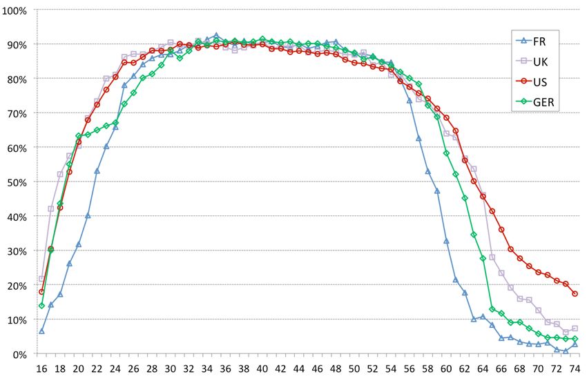
Tax rates, tax credits and work decisions
• This first (and main) section of this component of the course
  will analyse the impact of tax and benefit reform on work
  and earnings.
• It will look at the context, the impact and the design of
  reforms.
• It will focus on two questions:
   – How should we measure the impact of taxation on work
     decisions and earnings?
   – How should we assess the optimality of tax reforms?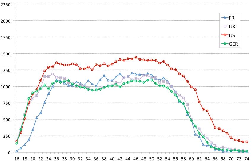
Why re-examine earnings taxation?
•    Changes in employment patterns, in earnings inequalities –
     covid-19?
•    New empirical findings on labour supply elasticities
•    New insights from optimal tax design theory
•    A need to look at the whole income tax/benefit system
     –   Key chapter (in Mirrlees Review): Brewer, Saez and
         Shephard.
     –   Minimum (National Living) wage and tax-credit debate.
•    References at the end of the lecture slides.
Changes in the economic environment
 • Changes in employment patterns
    – growth of female labour supply,
    – changes in ‘early retirement’ behaviour.
 • Changes in population
    – growth in single person & single parent households,
    – growth in migration.
 • Growth in earnings and wealth inequalities
    – growth in top income and wealth share.
    – fall in the relative earnings of the lower educated, especially the
      relative earnings of low skilled men.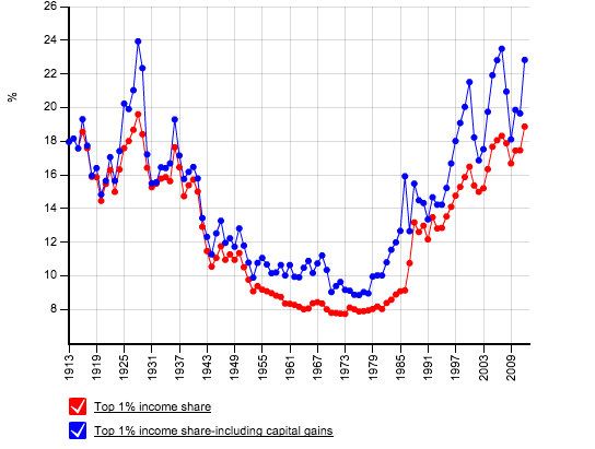
Top Income Shares in the US

     Source: Piketty and Saez (2013), Notes: World Top Incomes Database
Employment for men by age – FR, UK and US 2007
Blundell, Bozio and Laroque (2011)Total Hours for men by age – FR, UK and US 2007
Blundell, Bozio and Laroque (2011)Female Employment by age – US, FR and UK 2007
Blundell, Bozio and Laroque (2011)Female Total Hours by age – US, FR and UK 2007
Blundell, Bozio and Laroque (2011)Increased empirical knowledge
• labour supply responses for individuals and families
• at the intensive and extensive margins
– extensive margin elasticities generally higher than
intensive margin
• by age and demographic structure
– labour supply elasticities higher for mothers with
younger children and for pre-retirement adults
• taxable income elasticities
– top of the income distribution using tax return
informationThe taxation of income from earnings
• Examine the way taxes and welfare-benefits impact on
family income as individual earnings vary.
– Simple tax schedules are not necessarily the best for either
economic efficiency or for fairness.
• However, to be effective an earnings tax system has to
be understandable to employees and employers.
– To quote the Nobel prizewinner Herb Simon ‘..a wealth of
information creates a poverty of attention’.
• There is a therefore a balance between complexity and a
need for a transparent tax code.Measurement of effective tax rates
• Precisely how do tax policies impact on the incentives
facing the key players?
– overlapping taxes and employee contributions at the top,
– interacting tax credits and welfare benefits at the
bottom.
• What are the ‘true’ effective tax rates on (labor) earnings?Effective marginal rates for higher earners in the UK
Income tax schedule for those aged under 65, UK 2010–11
Source: Mirrlees Review (2011)For lower earners there are key interactions with
welfare benefits & tax credits
Budget Constraint for Single Parent in UK
£300.00
£250.00
Local tax rebate
£200.00 Rent rebate
WFTC
£150.00
Income Support
£100.00 Net earnings
Other income
£50.00
£0.00
0
5
10
15
20
25
30
35
40
45
50
hours of workMeasuring effective tax rates
• It is essential to assemble all the components of the tax schedule
and examine the system as a whole.
• One way to achieve this and to capture the complete picture of
the tax rate schedule is through the calculation of effective
marginal tax rates (MTR) and participation tax rates (PTR).
• The ‘effective marginal tax rate’ is the proportion of an £1 of
extra earnings retained in the tax and benefit system. This will
include all employer taxes and contributions as well as the full
set of taxes and benefits. It typically varies widely.
• By contrast the ‘effective participation tax rate’ is the net loss,
through taxes and benefits, of earnings in work relative to being
out of work.In the UK • Income Support, Rent and Housing Benefit etc., create high MTRs, PTRs • In-work tax-credits can reduce these high MTRs and PTRs for low-income workers • Let’s look at the design on of earned income tax credits in the US and UK.
The general form of Earned Income Tax Credits

 • Credit depends on earnings and number of
   children:
    – Phase-in: credit is flat percentage of earned
      income or jump in at minimum hours threshold
    – Flat range: receive maximum credit
    – Phase-out: credit is phased out at a flat rate
 • Credit based on family earnings
    – Creating ‘interesting’ incentives among
      couples
The EITC Schedule in US
Single Parent Families, 2004
$5,000
$4,000
EITC Credit
Flat Region
$3,000
Phase In
Region
$2,000
Phase-out
Region
$1,000
$0
$0 $5,000 $10,000 $15,000 $20,000 $25,000 $30,000 $35,000 $40,000
Earnings
Two or more children One Child
Ø Larger credit, covering higher earners for families
with two or more children.Universally Available Tax and Transfer Benefits in US Single Parent with Two Children, 2008 Source: Urban Institute (NTJ, Dec 2012). Notes: Value of tax and value transfer benefits for a single parent with two children.
Effective Marginal Tax Rates
  (US Single Parent with Two Children in Colorado, 2008)

Source: Urban Institute (NTJ, Dec 2012).
Notes: Value of tax and value transfer benefits for a single parent with two children.
Expenditure per Capita on Non-Medicaid Means Tested
Programs, US (real 2009 dollars)
                          300

                          250

                                                 AFDC/TANF
                          200
 Expenditure per Capita

                          150
                                       SSI
                                                                                               SNAP
                                                                                               (food stamps)
                          100
                                                                          EITC
                                               Housing Aid
                           50

                            0
                                1970    1975       1980      1985   1990         1995   2000   2005            2010
                                                                        Year

       Source: Moffitt (2017)
Number of EITC Recipient Families (Millions)
25
EITC Recipients (Millions)
20
15
10
5
0
1975 1980 1985 1990 1995 2000
Year
Source: Green Book, 2004, US Joint Committee on Taxation, Ways and Means CommitteeIn-work Credits in OECD Countries
Approximate
Maximum
Target Income Increase Phase-in Phase-out Hours
group (Euros) criterion
Belgium Individual 440 Yes Yes No
Canada, Quebec Families 3,150 Yes Yes No
Finland Individual 290 Yes Yes No
France Individual 230 Yes Yes No
Ireland Families 2,260 or more No Yes Yes
Netherlands Individual 920 Yes No No
New Zealand Families 7,800 No Yes Yes
New Zealand Families 780 per child No Yes Yes
UK Families 6,150 or more No Yes Yes
United States Families 4,000 Yes Yes No
Source: Owens (OECD, 2005) Table 3.EITC Reforms in the US
• In the US the EITC started in 1975 as modest “work
bonus”; made permanent in 1978
• Substantial expansions have taken place:
– 1986 Tax Reform Act: general expansion and indexed
for inflation
– 1990: general expansion and added separate schedule
for families with 2 or more children
– 1993: general expansion (larger expansion for families
with 2 or more children) and added EITC for childless
filers
– Recently back in the policy debate again to support
low earning families.US: EITC Benefit for Selected Tax Years
(B) Schedule for Family with 2+ Children
$4,000
1996 EITC
$3,500
$3,000
$2,500
EITC Credit (1996 $)
$2,000
1993 EITC
$1,500
1990 EITC
$1,000
1984 EITC
$500
$0
$0 $5,000 $10,000 $15,000 $20,000 $25,000 $30,000
Earnings (1996 $)Earned Income Tax Credit reforms in the UK
• Sequence of Tax Credit policies:
– FC (Family Credit) before 2000, expanded early in
1990s
– WFTC (Working Families Tax Credit) reform in
2000
– WTC (Working Tax Credit) and CTC (child tax
credit) reform in 2004
– UC (Universal Credit) – 2016 onwards, integration
of tax credits and other benefits…..Particular Features of the UK Working Tax Credit
• hours of work condition
– minimum hours rule - 16 hours per week
– an additional hours-contingent payment at 30 hours
• family eligibility
– children (in full time education or younger)
– adult credit plus amounts for each child
• income eligibility
– family net income below a certain threshold
– credit is tapered away at 55% (previously 70% under FC)UK: The Tax Credit Expansion in the 2000 Reform
transfers per week for a min. wage lone parent
£120 -
55%
WFTC
70%
0
0 10 20 30 40 50 60 70
Hours worked per week
Family Credit WFTCBudget Constraint for Single Parent: UK WFTC
£300.00
£250.00
Local tax rebate
£200.00 Rent rebate
WFTC
£150.00
Income Support
£100.00 Net earnings
Other income
£50.00
£0.00
0
5
10
15
20
25
30
35
40
45
hours of work 50Are the eligibility rules in WFTC salient?
Single Women (aged 18-45) - 2002
• Blundell and Shephard (2010)The UK and US tax credit systems compared
£6,000
£5,000
WFTC
£4,000
£3,000 EITC
£2,000
£1,000
£0
£0 £5,000 £10,000 £15,000 £20,000 £25,000
Gross income (£/year)Bunching at Tax Kinks and the EITC One child families: US Source: Saez (2010)
The Canadian Self Sufficiency Program (SSP) • Designed to answer the question: Do financial incentives encourage work among low skilled lone parents? • To encourage employment among welfare recipients, specifically single parents on welfare – 50% earnings supplement – as a tax credit – at least 30 hours per week job – On earnings up to an annual limit of $36000 • Provided to the individual, not the employer, as in EITC and WFTC. Note the experimental research design of the SSP • Well designed social experiment, RCT
Canadian Self Sufficiency Program
Budget Constraint for a Single Parent on Minimum Wage
2500
Income per Month ($1995)
2000
SSP
1500
1000
IA
500
0
0 5 10 15 20 25 30 35 40 45 50 55 60
Weekly Hours of Work
Income Assistance Self Sufficiency ProgramCanadian Self Sufficiency Program: RCT results
Monthly Employment Rate for a Single Parent with One Child BC
40
Monthly Employment Rate
35
30
25
20
15
10
-10 -8 -6 -4 -2 0 2 4 6 8 10 12 14 16
Months from Random Assignment
Controls ExperimentalsHow should we choose tax rates?
• Follow the ‘optimal tax design’ approach due to Mirrlees (1971).
• Taxation is an information problem. The government cannot measure
everything it needs to - it just sees whether people work and (possibly)
how much they earn.
• The government cannot observe effort, it cannot distinguish a high ability
person working few hours from a low ability person working a large
amount.
• In this framework a tax schedule is chosen that will maximise social
welfare and raise a required amount of revenue.
• A balance of redistributive aims with effort incentives. If it taxes the high
ability types too much they may choose to supply much less effort, thus we
need good estimates of labour supply elasticities.
36A Typical ‘Integrated’ Schedule: Optimal?
Post tax
income
‘phase-out’
subsidy or region
‘phase-in’
region break even point
Some ‘Income
Support’ – but
what form?
0
0
Pre-tax earningsStart with a simple progressive tax system
I. The choice of the top tax rate
• How should we tax the very rich?
• We consider the different ways in which a small increase in the top rate
affects social welfare.
• We assume that this top rate applies to earnings above a given level, and
we will refer to this level as the top bracket.
• There are three impacts on social welfare:
1. mechanical effect on tax revenue
2. behavioural response on tax revenue
3. welfare effect, and it is a loss to society. How large is this loss depends on
the redistributive tastes of the government.
39The choice of the top tax rate
1. With no behavioural response, increasing the top rate will increase
government revenue. This is the mechanical effect on tax revenue, and this
is a benefit to society, as the revenue can be used for government spending
or higher transfers.
2. Increasing the top rate may also induce top bracket taxpayers to reduce
their earnings (but not below the top bracket, because nothing has changed
below this point) because of the substitution effect described above. This is
known as the behavioural response on tax revenue, and it is a cost to
society as tax revenues will fall.
3. Finally, any increase in the top rate will reduce the welfare of top bracket
taxpayers. This is the welfare effect, and it is a loss to society. If the
government values redistribution, then, for incomes above a certain level,
it will consider that the marginal value of income is small. In the limit, the
welfare effect will be negligible relative to the mechanical effect on tax
revenue.
40The choice of the top tax rate
• Consider a reform that changes the top tax rate τ by a small amount
dτ
• Let z be the earned income being considered for taxation
• The top bracket begins at income z*
• Assume there are N taxpayers in the top bracket
1. Mechanical effect of higher marginal tax rate on incomes above z*:
dM = N[z – z*] dτ > 0
2. Behavioural effect will depend on the elasticity e – the elasticity of
earnings with respect to the net of tax rate (1- τ). Reported income
will be reduced by
dz = - e z dτ / (1- τ)
Hence revenue will be reduced by
dB = - N e z dτ τ / (1- τ)
41The choice of the top tax rate
• Suppose the government gives a value of g to an extra £1 to a top tax
bracket taxpayer – will be strictly less than 1, since the weighted
sum of welfare weights is unity.
3. Welfare effect of higher marginal tax rate on incomes above z*:
dW = - g N[z – z*] dτ < 0
Summing these we get
dM + dB + dW = N dτ [z – z*] [1 – g – e.a.τ / (1- τ)]
where a = z/(z – z*).
At the optimum this has to be zero
τ* = (1 – g) / (1 – g + a.e)
42The choice of the top tax rate
There are some very nice interpretations of this simple formula
τ* = (1 – g) / (1 – g + a.e)
1. Note that a is a parameter of the upper tail of the Pareto
distribution ( f(z) = C/z1+a ).
2. If g is approximately zero then
τ* = 1 / (1 + a.e)
which is very simple to estimate if we know the taxable income
elasticity.
For example, if e = .5 and a = 1.67,
then τ* = 1 / (1 + 1.67 .5) = .545
A revenue maximising top tax rate of approximately 55%.
3. But how do we measure ‘a’ and ‘e’?
43Pareto distribution as an approximation to the income distribution
0.0100
Pareto distribution
Probability density (log scale)
Actual income distribution
0.0010
0.0001
0.0000
0.0000
£100,000 £150,000 £200,000 £250,000 £300,000 £350,000 £400,000 £450,000 £500,000
Pareto parameter for the UK quite accurately estimated at 1.67Top incomes and taxable income elasticities: UK
A. Top 1% Income Share and MTR, 1962-2003
80% 16%
70%
14%
60%
Marginal Tax Rate
12%
Income Share
50% Top 1% MTR
Top 1% income share
40% 10%
30%
8%
20%
6%
10%
0% 4%
1962
1966
1970
1974
1978
1982
1986
1990
1994
1998
2002
Source: Brewer, Saez and Shephard (Mirrlees Review)B. Top 5-1% Income and MTR, 1962-2003
80% 16%
70%
14%
60%
Marginal Tax Rate
12%
Income Share
50%
40% 10%
30%
8%
20%
Top 5-1% MTR
6%
10% Top 5-1% income share
0% 4%
1962
1966
1970
1974
1978
1982
1986
1990
1994
1998
2002
46
Source: Brewer, Saez and Shephard (Mirrlees Review)Ex-post (quasi-experimental) estimation of elasticities
Abstracting from other regressors X, write the tax reform as a
binary indicator d and taxable income (or employment or hours)
as y, we write:
yit = b + a i di + uit
a i = a AT + e i
a TT = a AT + E (e i | di = 1)
Two parameters of interest:
ATE: Average (Treatment) Effect is given by αAT
ATT: Average (Treatment) Effect on the Treated is given by αTTDifference-in-Differences estimator (DiD)
Let yT and yC represent the mean outcomes for the treatment and
comparison (non-treatment) groups, respectively.
Let t=0 and t=1 represent the time period before and after policy
intervention.
The difference in differences estimator is given by:
a DD = ( y - y ) - ( y - y )
T
t =1
T
t =0
C
t =1
C
t =0Key Assumptions:
Common Trends and Time Invariant Composition
yit = b + a i di + uit
a i = a AT + e i
aTT = a AT + E (e i | di = 1)
Given the way we have expressed individual and time effects, we have
uit = fi + qt + µit
E (uit | di ) = E (fi | di ) + qt
E (a DD ) = [ b + a TT + E (ui ,t =1 | di = 1] - [ b + E (ui ,t =0 | di = 1]
- [ b + E (ui ,t =1 | di = 0] - [ b + E (ui ,t =0 | di = 0]
= aTT
That is, the ATT is identified by DiD, but not the average population
treatment impact.Taxable Income Elasticities at the Top in UK
Simple Difference DiD estimates
(top 1%) using top 5-1%
as control
1978 vs 1981 0.32 0.08
1986 vs 1989 0.38 0.41
1978 vs 1962 0.63 0.86
2003 vs 1978 0.89 0.64
Full time series 0.69 0.46
(0.12) (0.13)
• With updated data the estimate remains in the .35 - .55 range with a central
estimate of .46, but remain quite fragile
• Pareto parameter quite accurately estimated at 1.67, so the implications for
τ* = 1 / (1 + a.e) => revenue maximising tax rate for top 1% of around 56%.
• But note also the key relationship between the size of elasticity and the tax
base (Slemrod and Kopczuk, 2002)Bunching at the higher rate tax thresholds The case of the UK Source: Mirrlees Review
Composition of income around the higher rate tax threshold
=> measure taxable income elasticity
Source: Mirrlees ReviewMarginal tax rates by income level, UK 2007–08 Note: assumes dividend from company paying small companies’ rate. Includes income tax, employee and self-employed NICs and corporation tax.
Bunching at Tax Kinks and the EITC
One child families: US

Source: Saez (2010)
The taxable income elasticity e

• Topics for discussion:
• Has the elasticity e changed over time?
• Is the method for estimating e reliable?
• Is the Pareto distribution assumption a good one?
• How would a bargaining model change the arguments? (see
  Piketty, Saez and Stantcheva (2014)
Top tax rates and migration

• Concern that individuals move to low tax countries

   – migration response is similar to an extensive response

• Optimal top tax rate with migration elasticity (m) + intensive
  elasticity (e) is given by:
                MTR=1/(1+a·e + m)

   – does the migration elasticity change in recessions?
   – the nature of evidence on migration elasticity ‘m’ is weak.
II. The general tax schedule
• How should we tax lower incomes?
• Again we consider the different ways in which a small increase
in the rate at any point in the earnings distribution affects social
welfare.
• We begin by allowing the tax and benefit system to be fully
‘non-linear’, which means that marginal tax rates at a particular
point of the earnings distribution can be set to any value
without altering marginal rates at other points.What about the general tax schedule? • The optimal MTR at any point is set so as to balance the costs and benefits from changing the MTR by a very small amount. • As before, an increase in the MTR over a very small band of income has three effects on government tax receipts and welfare: 1. the mechanical effect 2. the behavioural effect generates a loss in tax revenue 3. a welfare cost whose size will depend upon the extent to which the government values redistribution.
The optimal marginal tax rate schedule
•    For income z, denote T(z) as the tax function, H(z) as the
     cumulative distribution of individuals & h(z) is the density.
•    The optimal tax system is characterised by a lumpsum grant given to
     those without earned incomes – T(0), combined with a schedule of
     marginal rates T'(z).
•    Consider a reform that changes the marginal tax rate T'(z) by dτ in a
     small band of income (z, z + dz).
1.   The reform increases tax revenues by dτ.dz for every taxpayer above
     the small band, the mechanical effect is:
                       dM = (1 – H(z)).dz.dτ
The optimal marginal tax rate schedule
2. Those extra taxes also generate a welfare cost.
Let G(z) be the average social value of distributing £1
uniformly among taxpayers with income above z. The
welfare cost is
dW = dM.G(z)
3. The marginal tax rate increase dτ reduces earnings by
dz = - e.z.dτ / (1- T'(z))
There are h(z)dz such taxpayers, hence revenue will be
reduced by the behavioural effect
dB = - e.z.[ T'(z)/(1- T'(z))] dτ.h(z).dzThe optimal marginal tax rate schedule
At the optimum all these must sum to zero
dM + dW + dB = 0
Consequently, at the optimum
T'(z)/(1- T'(z))] = 1/e . (1-H(z))/h(z)z . (1-G(z))
1. The optimal tax rate decreases with the elasticity e.
2. It is also decreasing in G(z) which measures the
marginal value placed on income for individuals above z.
3. It is also decreasing in the hazard ratio zh(z)/(1-H(z))
which measures the thinness of the distribution.Negative marginal tax rates?
• It is worth noting that, in this framework, negative MTRs
are never optimal:
– if the MTR were negative in some range, then increasing it a
little bit in that range would raise revenue (and lower the
earnings of taxpayers in that range), but the behavioural
response (which would be to work less) would also be to raise
revenue, because the marginal tax rate is negative in that
range.
• Therefore, this small tax rise would unambiguously
increase social welfare.
• All this changes when we introduce a participation or
‘extensive’ margin of labour supply response.The importance of the extensive margin • With participation effects, the optimal tax formula changes. • Negative tax rates become possible and can justify earned income tax credit policies. • Labour supply estimation suggest extensive margin is more responsive to incentives than intensive margin • High marginal tax rates at the bottom are no longer necessarily desirable and negative participation tax rates can be optimal
Notes on the extensive margin:
•   If an individual decides to work he or she gets z - T(z).
•   If she decides not to work she will get –T(0).
•   Suppose utility was simply u = c – q where c is
    disposable income and q are costs of work.
•   Cost of work are distributed with a cumulative
    distribution P(q|z)
•   Define the elasticity of participation (extensive margin
    elasticity) as:
                          z − T (z) + T (0) ∂P
                       η=
                                  P         ∂q
Notes on the extensive margin (2)
• With participation effects, the optimal tax formula changes. Suppose
we allow taxes to be different across I different earnings levels. Then
the optimal structure has the form
Ti - Ti -1 1 I é T j - T0 ù
=
ci - ci -1 ei hi
å h j ê1 - g j - h j ú.
c j - c0 úû
j ³i êë
• Labour supply estimation suggest extensive margin is more
responsive to incentives than intensive margin
• High marginal tax rates at the bottom are no longer necessarily
desirable and negative participation tax rates can be optimal (Brewer,
Saez and Shephard (2012), Saez, 2002; Laroque, 2004).A Typical ‘Integrated’ Optimal Schedule
After Tax
Income
‘phase-out’
subsidy or region
‘phase-in’
region break even point
Some ‘Income
Support’ – but
what form?
0
0
EarningsImplications for Tax Reform
• Change transfer/tax rate structure to match lessons from ‘new’
optimal tax analysis and empirical evidence,
– the Mirrlees Review used a similar design framework for family
labour supply and early retirement.
• Key role of labour supply responses at the extensive and
intensive margins.
• Both matter but differ by gender, age, education and family
composition,
– lone parents, married parents, pre-retirement low earners.
• Results for lone parents suggest lower marginal rates at the
bottom,
– means-testing should be less aggressive,
– at least for some key groups where elasticities are relatively
high.Implications for Tax Reform
• ‘Life-cycle’ view of taxation
– distinguish by age of (youngest) child for mothers/parents
– pre-retirement ages
– effectively redistributing across the life-cycle
– a ‘life-cycle’ rearrangement of tax incentives and welfare
payments to match elasticities and early years investments
– results in Tax by Design show significant employment and
earnings increases
• Hours rules? – at full time for older kids,
– welfare gains depend on ability to monitor hours
• Dynamics and Human Capital
– little in the way of experience effects for low-skilled,
– complementarity with educational qualifications.Dynamic effects on wages for low income welfare
recipients?
SSP: Hourly wages by months after RA
8.5 8
Hourly real wages
6.5 7 6 7.5
0 10 20 30 40 50 60
Months after random assignment
control experimental
© Institute for Fiscal Studies400 SSP: Monthly earnings by months after RA
Monthly earnings
200 100 300
0 10 20 30 40 50 60
Months after random assignment
control experimental
© Institute for Fiscal StudiesImplications for efficient redesign of earnings taxation
• Target work incentives where they are most effective
– simulations in Mirrlees et al (2011) show increase in
work/earnings
– reducing means-testing and improving the flows into work for
lower education mothers and maintaining work for those aged
55+.
• Limits to tax rate rises at the top without tax base reform.
• Reduce disincentives at key margins for the educated
– enhancing working lifetime and the career earnings profile
– simulations in BDMS (2014) show significant on human capital.
• How should we think about the minimum/living wage and
incidence? – Rothstein (2010).Some References: see also course moodle page. Blundell, R. (2012) "Tax Policy Reform: The Role of Empirical Evidence," Journal of the European Economic Association, 10 (1), 43-77, 02, Blundell, R., Bozio, A. and Laroque, G. (2011), ‘Labour Supply and the Extensive Margin’, American Economic Review, Volume 101, Issue 3, May, 482-486. Blundell, R., M. Costa-Dias, C. Meghir and J. Shaw (2016), “Female Labour Supply, Human Capital and Welfare Reform”, Econometrica. Blundell, R, Duncan, A, McCrae, J and Meghir, C. (2000), "The Labour Market Impact of the Working Families' Tax Credit", Fiscal Studies, 21(1). Blundell, R. and Hoynes, H. (2004), "In-Work Benefit Reform and the Labour Market", in Richard Blundell, David Card and Richard .B. Freeman (eds) Seeking a Premier League Economy. Chicago: University of Chicago Press. Blundell, R. and A. Shephard (2012) "Employment, Hours of Work and the Optimal Taxation of Low-Income Families," Review of Economic Studies, vol. 79(2), pp 48-510. Key Reference: Brewer, M, E Saez, and A Shephard (2010) “Means-testing and Tax Rates on Earnings.” Mirrlees Review: Dimensions of Tax Design, ed. James Mirrlees, 90–173. Oxford University Press.
Card, D and P K. Robins (1998), "Do Financial Incentives Encourage Welfare
Recipients To Work?", Research in Labor Economics, 17, pp 1-56.
Card, D and D. Hyslop (2005), 'Estimating the Dynamic Treatment Effects of an
Earnings Subsidy for Welfare-Leavers' (with David Card), Econometrica, 73, 6 pp.
1723-1770.
Diamond, P. (1980): "Income Taxation with Fixed Hours of Work," Journal of
Public Economics, 13, 101-110.
Eissa, N. and J. Liebman (1996), "Labor Supply Response to the Earned Income
Tax Credit", Quarterly Journal of Economics, CXI, 605-637.
Gruber, J., and Saez, E. (2002) “The Elasticity of Taxable Income: Evidence and
Implications”, Journal of Public Economics, 84, 1-32.
Immervoll, H., H. Kleven, C. Kreiner, and E. Saez (2007): “Welfare Reform in
European Countries: A Microsimulation Analysis,” Economic Journal, 117, 1–44.
Brewer, M. A. Duncan, A. Shephard, M-J Suárez, (2006), “Did the Working
Families Tax Credit Work?”, Labour Economics, 13(6), 699-720.
Mirrlees, J.A. (1971), “The Theory of Optimal Income Taxation”, Review of
Economic Studies, 38, 175-208.
Rothstein, J. "Is the EITC as Good as an NIT? Conditional Cash Transfers and Tax
Incidence." American Economic Journal: Economic Policy 2 (1), February 2010, p.p.
177-208.
Saez, E. (2002): "Optimal Income Transfer Programs: Intensive versus Extensive
Labor Supply Responses," Quarterly Journal of Economics, 117, 1039-1073.
Saez, E. (2010) “Do Taxpayers Bunch at Kink Points?”, AEJ: Economic Policy, Vol.
2, 180-212.
Saez, E., J. Slemrod, and S. Giertz (2012) “The Elasticity of Taxable Income with
Respect to Marginal Tax Rates”, Journal of Economic Literature 50(1), 3-50.
Piketty, T, E Saez, and S Stantcheva (2014) “Optimal Taxation of Top Incomes: A
Tale of Three Elasticities.” American Economic Journal: Economic Policy 6 (1): 230-
271.
Slemrod, J. and W. Kopczuk (2002), “The optimal elasticity of taxable income”,
Journal of Public Economics 84 (2002) 91 –112
Employment for men by age – FR, UK, US & GER 2007

                        •   Blundell, Bozio, Laroque and Peichl (2014)
Total Hours for men by age – FR, UK and US 2007
Blundell, Bozio and Laroque (2011)Total Hours for men by age – FR, UK and US 1977
Blundell, Bozio and Laroque (2011)• For women earnings are influenced by taxes and benefits not
only at these margins but also when there are young children in
the family.
– for women with younger children it is not usually just an
employment decision that is important it is also whether to
work part-time or full-time.
• Often the employment margin is referred to as the extensive
margin of work and the part-time or hours of work decisions
more generally as the intensive margin.Female Employment by age - 2007
• Blundell, Bozio, Laroque and Peichl (2014)Female Hours by age
• Blundell, Bozio, Laroque and Peichl (2014)and for women …..
Female Employment by age – US, FR and UK 1977
Blundell, Bozio and Laroque (2011)You can also read