Dynamical Data Mining Captures Disc-Halo Couplings that Structure Galaxies - arXiv
←
→
Page content transcription
If your browser does not render page correctly, please read the page content below
MNRAS 000, 000–000 (2023)                          Preprint 9 January 2023            Compiled using MNRAS LATEX style file v3.0

                                              Dynamical Data Mining Captures Disc-Halo Couplings
                                              that Structure Galaxies
                                              Alexander Johnson1⋆ , Michael S. Petersen2 , Kathryn V. Johnston1,3 , Martin D. Weinberg4
                                              1 Department   of Astronomy, Columbia University, 550 West 120th Street, New York, NY 10027, USA
                                              2 Institutefor Astronomy, University of Edinburgh, Royal Observatory, Blackford Hill, Edinburgh EH9 3HJ, UK
                                              3 Center for Computational Astrophysics, Flatiron Institute, 162 5th Av., New York City, NY 10010, USA
arXiv:2301.02256v1 [astro-ph.GA] 5 Jan 2023

                                              4 Department of Astronomy, University of Massachusetts, Amherst MA 01003-9305, USA

                                              9 January 2023

                                              ABSTRACT
                                              Studying coupling between different galactic components is a challenging problem in galactic dynamics. Using basis
                                              function expansions (BFEs) and multichannel singular spectrum analysis (mSSA) as a means of dynamical data
                                              mining, we discover evidence for two multi-component disc-halo dipole modes in a Milky-Way-like simulated galaxy.
                                              One of the modes grows throughout the simulation, while the other decays throughout the simulation. The multi-
                                              component disc-halo modes are driven primarily by the halo, and have implications for the structural evolution of
                                              galaxies, including observations of lopsidedness and other non-axisymmetric structure. In our simulation, the modes
                                              create surface density features up to 10 per cent relative to the equilibrium model stellar disc. While the simulated
                                              galaxy was constructed to be in equilibrium, BFE+mSSA also uncovered evidence of persistent periodic signals incited
                                              by aphysical initial conditions disequilibrium, including rings and weak two-armed spirals, both at the 1 per cent level.
                                              The method is sensitive to distinct evolutionary features at and even below the 1 per cent level of surface density
                                              variation. The use of mSSA produced clean signals for both modes and disequilibrium, efficiently removing variance
                                              owing to estimator noise from the input BFE time series. The discovery of multi-component halo-disc modes is strong
                                              motivation for application of BFE+mSSA to the rich zoo of dynamics of multi-component interacting galaxies.

                                              1 INTRODUCTION                                                         Recent work by Weinberg & Petersen (2021) suggest one
                                                                                                                  approach to this challenge centred around two mathemat-
                                              The structures of galaxies are manifestations of how the laws       ical tools: Basis Function Expansions (BFE) and Multi-
                                              that govern dynamics combine with the nature of matter. Un-         Channel Singular Spectrum Analysis (mSSA). BFE rep-
                                              derstanding galaxies strengthens our understanding of fun-          resent a distribution as a linear combination of basis
                                              damental physics. There are tremendous opportunities to             functions, with half a century of application to galac-
                                              deepen that understanding: a rich legacy of analytic descrip-       tic dynamics (e.g. Clutton-Brock 1972, 1973; Kalnajs
                                              tions of galactic dynamics; community investment in high            1976; Polyachenko & Shukhman 1981; Weinberg 1989, 1999;
                                              resolution simulations; large scale, high dimensional surveys       Petersen et al. 2022). When representing a simulation with a
                                              of billions of stars and galaxies; and the emergence of the         fixed set of basis functions, one obtains time series of co-
                                              vital field of data science to robustly mine and characterise       efficients that encode the dynamics in a compressed rep-
                                              both simulated and real data sets.                                  resentation. mSSA is a method for identifying temporal
                                                 Yet recent years have revealed the limits to our conception      correlations. Together, one obtains a powerful analysis tool
                                              of our home galaxy, long thought to be a quiet backwater in         for studying galaxy simulations. The method does not re-
                                              the Universe. Maps of the positions and motions of billions of      quire prior information and thus can be considered a form of
                                              stars from the Gaia satellite (Gaia Collaboration et al. 2016,      unsupervised learning. Applying mSSA to BFE time-series,
                                              2018, 2022) have revealed a Milky Way in disarray, with abun-       Weinberg & Petersen (2021) analysed barred-galaxy simula-
                                              dant signatures of action and reaction - past and ongoing           tions. They found that BFE+mSSA could autonomously ex-
                                              (e.g. Antoja et al. 2018; Trick et al. 2019; Friske & Schönrich    tract the dominant space and time correlated features and
                                              2019; Helmi 2020). These represent significant departures           disentangle different phase of bar formation and evolution
                                              from the descriptions of equilibrium and mild perturbations         recovered through more traditional analysis (Petersen et al.
                                              on which the field of Galactic Dynamics has been built              2021).
                                              (Binney & Tremaine 2008). Simulations are capable of cap-
                                              turing such complexities but robustly linking the features to         In this paper, we build on the success of
                                              theoretical descriptions and identifying their physical origins     Weinberg & Petersen (2021) in characterising the evo-
                                              remains challenging.                                                lution of a known feature and explore the use of BFE+mSSA

                                              © 2023 The Authors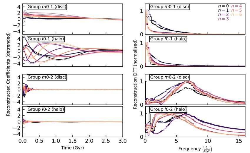
2     A. Johnson et al.
as a dynamical discovery tool. We do so through the analysis
of a model galaxy comprised of a stellar disc, stellar bulge,
and dark matter halo that is designed to be in equilibrium
and hence featureless (described in Section 2). Studying
such a galaxy serves as a ‘control’ sample for future work
with more feature-rich discs, with features from in situ (i.e.
spiral arms) or ex situ (i.e. minor mergers) sources. With a
control model, we want to answer the following questions
about BFE+mSSA as a dynamical data mining tool:
1) Can BFE+mSSA separate distinct features that overlap in
time and are not distinct by eye (real astrophysical signals,
phase mixing, and N -body noise)?
2) Can BFE+mSSA connect features within or across
components by identifying their shared spatial and temporal
structure?
The answer, as we shall see, is yes to both questions.
BFE+mSSA isolates features and allows them to be in-
terpreted independently, while also isolating interactions         Figure 1. Circular (black) and radial (red) frequency curves as a
between components independent of the presence of other            function of radius for the T = 0 equilibrium model. Both frequen-
interactions.                                                      cies are computed using the epicyclic approximation, in the plane
   While analysing the disc in the present study, it became        of the disc (z = 0). Three frequency values have been marked to
clear that the model was not the perfect featureless system we     guide the eye (Ω = 0.6, Ω = 1.5, and Ω = 6.6 cycles/Gyr), cor-
intended. By applying BFE+mSSA to the disc, and then the           responding to spatial scales near the peak disc circular velocity
combination of disc+halo, we identify two dynamical causes         (2.2Rd = 7.7) and multiples of the halo scale length (a = 52 kpc).
of features: phase-mixing from initial conditions, and interac-
tions between the disc and halo. We identify multiple distinct
dynamical signals in each, and examine the dynamical signals       cillations that lead to a self-similarly growing or damping
in detail (Section 3). We find that the signals are likely to be   response to a perturbation1 .
generic features in disc+halo systems, and can have real im-          Continuous modes are excited by perturbations with
pact on galaxies in the real Universe.                             a continuous range of frequencies, for example a single en-
   This study is a key step in understanding and exploring the     counter with a satellite. Other sources of disequilibrium,
strengths and limitations of BFE+mSSA in multi-component           whether physical or aphysical, also drive continuous response.
systems (see Section 4). In partnership, BFE+mSSA has              This continuous response appears as phase mixing in galax-
great potential beyond simulations analysis. Much of analytic      ies. These modes are also transient: since the response is not
linear theory is also built on BFEs. Moreover BFEs may be          dominated by a single frequency the mode quickly looses co-
used to described observational data sets. Hence BFEs pro-         herence and therefore is not self-sustaining. We expect that
vide a common dynamical language to quantitatively con-            mSSA will efficiently detect a plethora of signals owing to
nect theory, simulations, observations and data science while      continuous modes, of varying strength. These signals will ap-
providing rigorous physical interpretations of dynamical pro-      pear with relatively broad frequency support. As the modes
cesses. We conclude in Section 5 with a discussion of how          are transient, few theoretical approaches exist capable of pre-
our results impact galaxy evolution more generally, and how        dicting the existence or evolution of these modes, making
BFE+mSSA fits in a larger program of dynamical data min-           BFE+mSSA an efficient tool to study them.
ing.                                                                  Point modes are excited by specific frequencies. They
                                                                   have model-dependent self-similar shapes and well defined
                                                                   frequencies and can therefore be reinforced by their own
                                                                   gravity. The point modes are damped (growing) for sta-
                                                                   ble (unstable) systems. The most commonly known point
2 METHODS                                                          mode is the Jeans’ instability in a homogeneous sea of stars
We first review the rationale and overarching goals for            (e.g. Binney & Tremaine 2008). Fluctuations from environ-
BFE+mSSA analysis in dynamical systems in Section 2.1,             mental disturbances such as satellite encounters or Poisson
and then describe the construction of a model isolated             noise from N -body distributions may excite these weakly
disc+bulge+halo galaxy in Section 2.2. Two appendices pro-         self-gravitating features. We expect that some of the results
vide specifics of the expansions used in our analysis (Ap-         recovered by mSSA will be the phase space manifestation
pendix B) and an overview of mSSA (Appendix C).                    of these modes, appearing as distinct frequency peaks. Cal-
                                                                   culations for unstable evolutionary modes in galactic discs

2.1 Rationale for BFE+mSSA analysis                                1  Mathematically, we are referring to the set of solutions to the col-
                                                                   lisionless Boltzmann equation for at a specific complex frequency.
All self-gravitating stellar systems, like ionised plasma,         These are the solutions to the response operator that generalise
have a spectrum of both continuous and point modes                 eigenfunctions in a finite vector space. In plasma physics, these
(Krall & Trivelpiece 1973; Ichimaru 1973; Ikeuchi et al.           solutions are usually call ‘modes’ although there is some disagree-
1974). Here, we define a mode to be a superposition of os-         ment.

MNRAS 000, 000–000 (2023)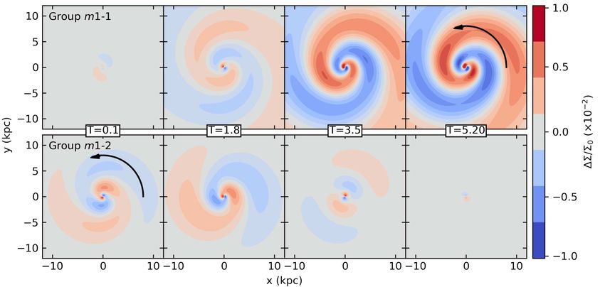
Near-equilibrium disc-halo dynamics                    3
                                                                         the disc plane are shown in Figure 1: as we shall see below, we
                                                                         are able to use these frequencies to inform our mSSA analy-
                                                                         sis. We evolve the model with Gadget-4 (Springel et al. 2021)
                                                                         for 5.49 Gyr, saving snapshots every 0.01 Gyr, for a total of
                                                                         549 snapshots. The total simulation requires approximately
                                                                         800 GB of computer disk storage.

                                                                         2.2.2 BFE representation
                                                                         To compactly describe the simulation, we represent each com-
                                                                         ponent in each snapshot with a BFE designed to provide
                                                                         compression and create a continuous representation from the
                                                                         particles. Further information regarding the BFEs used may
                                                                         be found in Appendix B. In a BFE, a target distribution is
                                                                         represented as the linear sum of some chosen basis functions,
                                                                         with weighting on each of the basis functions (coefficients).
Figure 2. Disc coefficients over time for the first three harmonic       If the basis functions are selected well, the distribution will
orders (m = 0, 1, 2) and all corresponding radial orders (n ∈ [0, 6]).   be described by a small number of functions and correspond-
The coefficients have been detrended by subtracting the mean and         ing coefficients, Cµ , where µ is a tag that indexes each basis
dividing out the variance. The coefficient series are dominated by       function. The coefficients then are a measure of the impor-
apparent noise, though some trends may be discerned: a steady            tance of each basis function to representing the overall dis-
decrease in some m = 0 coefficients (upper panel), elevated am-          tribution. To facilitate representing the distribution with the
plitude towards the end of the simulation in m = 1, and some             smallest number of functions, we choose expansions whose
periodicity in m = 2. The origin of these features is difficult to
                                                                         lowest-order function resembles the target equilibrium.
interpret owing to the coefficient series’ noisy appearance across
multiple basis functions. Any spatial features encoded in the basis         For a principally two-dimensional structure, the stellar
are all but impossible to determine.                                     disc, we use a Fourier-Laguerre expansion3 . The Fourier-
                                                                         Laguerre basis for expanding disc surface density was intro-
                                                                         duced in Weinberg & Petersen (2021). Given the exponential
have found evidence for point modes supported in various                 weighting of Laguerre polynomials, they serve as a natural
analytic geometries (e.g. Fouvry et al. 2015; De Rijcke et al.           radial basis element for exponential discs. If the scale lengths
2019). While we do not have explicit theoretical results for             are chosen to match, the equilibrium disc is well-represented
damped modes at many azimuthal orders in discs, N -body                  by the lowest-order Laguerre polynomials. The scale length
simulations seem to suggest that the amplitude is largest at             of our Fourier-Laguerre expansion is 3.5 kpc, matching the
m = 2 and decreases for m > 2. Crucially for the problem at              scale length of the modelled disc. To capture angular struc-
hand (a disc+halo system), we have no analytic predictions               ture, we expand in Fourier terms cos φ and sin φ. We in-
for the modal spectra, owing to the complexity of approaching            dex the Fourier azimuthal with m, and the Laguerre radial
such a problem analytically. BFE+mSSA gives us a means to                terms with n, creating (2m − 1) × n total coefficients, each
detect these modes amongst a sea of other signals.                       tagged with a unique (m, n), written Cmn . We find that as
                                                                         expected, C00 dominates by multiple orders of magnitude as
                                                                         desired. We expand the disc to mmax = 6, nmax = 6, making
2.2 Model Galaxy                                                         2 × (mmax + 1) × nmax = 84 coefficients for the disc. The
2.2.1 Simulation Overview                                                choice of maximum radial order is motivated by a desire to
                                                                         probe specific spatial scales. The n = 6 radial Laguerre den-
We design an isolated model Milky-Way-like galaxy for our                sity function has nodes at 0.9, 3.1, 6.8, 12.1, 19.7, and 30.9
study of the compressive power2 of BFE and the dynamical                 kpc, thus ensuring that the majority of the nodes are within
information one can extract with mSSA. We draw the model                 18 kpc of the disc centre (where 90% of the particles are
from components in the merger simulation of Laporte et al.               located).
(2018): a Hernquist profile dark matter halo with a mass of                 The dark matter halo4 is efficiently described through the
1012 M⊙ and a scale length of 52 kpc; an exponential stellar             empirical orthogonal function basis approach introduced in
disc with a mass of 6 × 10¹⁰ M⊙ , a scale length of 3.5 kpc, and         Weinberg (1999) and most recently updated in Petersen et al.
a sech2 scale height of 0.53 kpc; a Hernquist stellar bulge with
a mass of 1010 M⊙ and a scale length of 0.7 kpc. The halo has
40×106 particles, the disc has 5×10⁶ particles, and the bulge            3 Another option is presented in Weinberg & Petersen (2021): the
has 106 particles. Unlike Laporte et al. (2018), we do not in-           use of 3d basis functions designed to resemble the exponential
troduce a satellite perturber so that our model galaxy evolves           disc. In this work, we use the 2d Fourier-Laguerre expansion owing
in isolation. The initial circular and radial frequency curves in        to the straightforward generalisation to the expansion of velocity
                                                                         fields, which will be the subject of future works.
                                                                         4 We also tested bulge expansions, using a similar basis to the
2 Here, ‘compression’ refers to the amount of information one            dark matter halo. Tests indicated that information contained in
needs to store. A straightforward metric is the total computer disk      the bulge basis was redundant with the dark matter halo: this
space. We provide specifics to our simulation, but the scale of com-     makes sense for two spherical components. Therefore, we omit the
pression should be similar in other simulations.                         bulge expansion from the analysis in the rest of the paper.

                                                                                                             MNRAS 000, 000–000 (2023)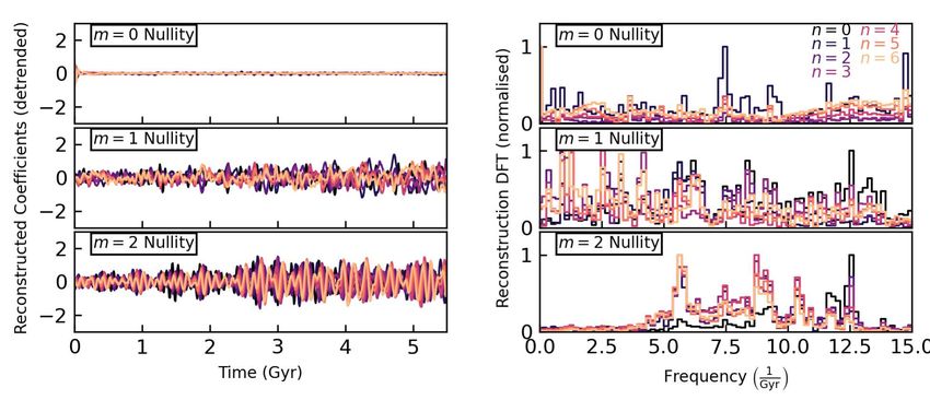
4     A. Johnson et al.
                                                      mSSA                         DFT peak        contrast       SV
                             name                 decomposition            PCs      (Gyr−1 )      (R < Rd )    fraction

                                      Disequilibrium Signal 1: halo profile readjustment (slow decay)

                          Group m0-1                disc m = 0             0,1         0.2          0.031       0.641
                          Group l0-1                halo l = 0           0,1,2,3       0.4            -         0.944
                         Group m0l0-1         disc m = 0, halo l = 0     0,1,2,3       0.2          0.054       0.832

                               Disequilibrium Signal 2: phase mixing of disc initial conditions (fast decay)

                         Group m0-2                 disc m = 0           2,3,4,5       6.4          0.006       0.084
                         Group l0-2                  halo l = 0            4,5         6.6            -         0.028
                        Group m0l0-2          disc m = 0, halo l = 0       4,5         6.6          0.007       0.037
                         Group m1-3                 disc m = 1             4,5         6.9          0.002       0.057
                         Group m2-1                 disc m = 2             0,1         6.6          0.006       0.201
                         Group m4-1                 disc m = 4             0,1         14.2         0.004       0.086
                         Group m6-1                 disc m = 6             0,1         20.2         0.001       0.036
                      Group m2m4m6-1              disc m = 2, 4, 6         0,1         6.6          0.010       0.072
                       Group m1l1-3           disc m = 1, halo l = 1       6,7         6.9          0.002       0.040
                      Group m1m2l1-2         disc m = 1, 2, halo l = 1     2,3         6.6          0.003       0.082
Table 1. Summary of two different signals identified in our mSSA decompositions as associated with initial disequilibrium. The first
signal results from halo disequilibrium, and the appearance in the disc is primarily manifest in the central surface density. The second
signal is present in myriad decompositions, but appears to be seeded first by disequilibrium in the disc m = 0, which then persists in other
harmonics. Disc feature strengths are reported in surface density to give a measure of ‘visual contrast’, defined as max (|∆Σ |) within a disc
scale length (see equation C9). Contrasts have an approximate error of 0.001, estimated from grid size adjustments. Owing to simulation
sampling rates (0.01 Gyr), the DFT peak is only accurate to 0.1.

(2022). Beginning with the equilibrium distributions, we de-             signals buried in the higher frequency noise: early evolution
sign a 1d radial model that matches the initial spherically              in m = 0; modestly elevated power at late times in m = 1;
symmetric density profile. From this one-dimensional model,              and a periodic signal in m = 2.
we construct an empirical orthogonal function basis whose                   To explore dynamical evolution in our simulation, we per-
lowest-order member perfectly matches the input initial den-             formed mSSA decompositions of various combinations of
sity profile. Higher-order terms are generated as eigenfunc-             BFE coefficients. These decompositions revealed clean, per-
tions of the Sturm-Liouville equation with the input equi-               sistent features in the individual low-order disc harmonics
librium potential-density model and appropriate boundary                 (m = 0, 1, 2), which we concentrate on understanding in this
conditions. The three-dimensional structure of the spherical             section. We also augment the analysis of the low-order disc
components is described by a spherical harmonic expansion                harmonics with mSSA analysis of halo coefficients, joins of
in the angular coordinates. Each term in the expansion is rep-           disc and halo coefficients, and higher-order disc harmonics
resented by three numbers: the spherical harmonic indices ℓ              (m > 2). These multi-component mSSA analyses prove to
and |m| ≤ ℓ and the index of the radial basis function n. In             be the most fruitful in identifying the causes of different fea-
total, we have (ℓmax + 1)2 × nmax coefficients per snapshot.             tures. The full results of all our analyses are presented in
For the halo, we expand to ℓmax = 2, nmax = 11. The expan-               Appendix A.
sions, for the entire simulation, only require approximately 12             Section 3.1 describes how the results of the mSSA analysis
MB of storage: a more than 60000× compression, with the                  can be used to group coefficients into separate dynamical fea-
benefit of encoding the dynamics. In practice, we will often             tures, characterise the properties of these features and come
consolidate the same-integer positive and negative spherical             to a physical understanding of their nature. The following
harmonic m indices when describing the coefficient ampli-                subsections illustrate these ideas by dividing our own anal-
tudes such that a quoted (ℓ, m) tag contains both ±m. As                 ysis of the disc+bulge+halo simulation into three classifica-
expected, the Cℓmn = C000 term is the largest by multiple                tions: initial conditions disequilibrium (Section 3.2), secular
orders of magnitude, with C generally decreasing as either               evolution signals (Section 3.3), and fluctuations and other
(ℓ, m) or n increases.                                                   uninterpretable features (Section 3.4).

                                                                         3.1 Interpreting the results of the mSSA analysis
3 EVOLUTION OF A NEAR-EQUILIBRIUM
                                                                         We use several diagnostics (denoted below in slanted text)
  GALAXY
                                                                         to describe the character and understand the nature of the
Our isolated disc+bulge+halo galaxy was constructed to be                features identified in the mSSA analysis. Each diagnostic has
in a completely stable equilibrium. However, the model is                a corresponding section in Appendix C describing the math-
not in equilibrium, for reasons both physical and unphysical.            ematical details.
Figure 2 shows the raw BFE coefficients for the low-order                   Applied to BFE multiple series, mSSA identifies temporally
disc harmonics derived from the simulation snapshots. While              correlated signals in the BFE coefficients series as an ensem-
it is clear that the coefficient time-series are noisy, inspection       ble. Briefly, mSSA uses the autocorrelation of time lagged ma-
by eye suggests that there exists lower frequency coherent               trix of the input series and performs an eigenanalysis to find

MNRAS 000, 000–000 (2023)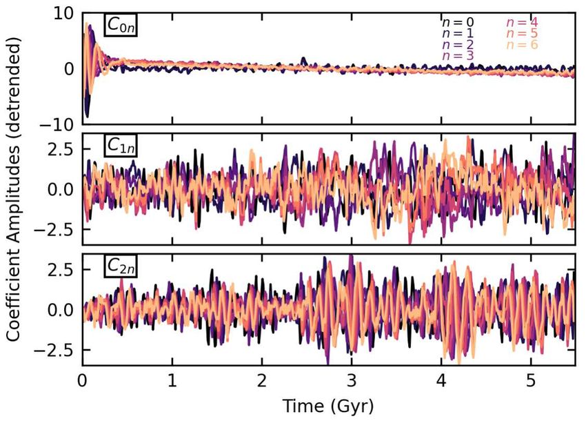
Near-equilibrium disc-halo dynamics 5
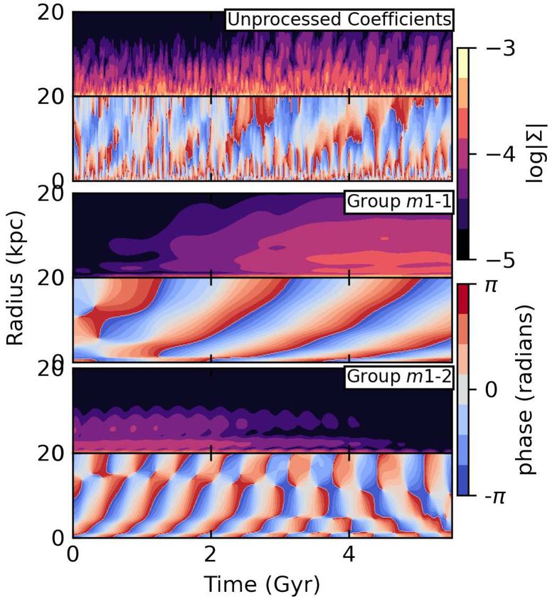
Figure 3. An analysis of two monopole signals resulting from distinct sources of initial disequilibrium. The left panels show the recon-
structed coefficient amplitudes over time for each signal (identified as Groups 1 and 2 in both disc-only, halo-only, and disc+halo analyses).
The right panels show the power spectra of the reconstructed coefficients for each group. The first signal is a slow rearrangement owing to
the halo settling in the presence of the disc, manifest by eye in the disc primarily as a change in the central surface density (cf. Figure 4).
We show the appearance of this signal in the disc and halo as the upper two rows. The second signal is ringing in the disc resulting
from the initial velocity disequilibrium of the disc. While the signal decays rapidly in the monopole component, the disequilibrium seeds
long-lasting persistent periodic features in other harmonics: see entries under ‘Disequilibrium Signal 2’ in Table 1. We show the appearance
of this signal in the disc and halo as the lower two rows. In each left-hand panel, we show two thicknesses of curves: the thick lines are for
the components when analysed separately and the thin lines are for the components when analysed jointly. That the different thicknesses
of lines, for the same radial order, are not particularly different, is strong evidence that the features are correlated between the disc and
halo.
mSSA DFT peak contrast singular value
name decomposition PCs (Gyr−1 ) (R < Rd ) fraction
Point Mode 1: slow growth
Group m1-1 disc m = 1 0,1 0.6 0.007 0.201
Group l1-1 halo l = 1 0,1,2,3 0.4 - 0.272
Group m1l1-1 disc m = 1, halo l = 1 0,1,2,3 0.6 0.008 0.244
Point Mode 2: slow decay
Group m1-2 disc m = 1 2,3 1.7 0.003 0.064
Group l1-2 halo l = 1 4,5 1.5 - 0.035
Group m1l1-2 disc m = 1, halo l = 1 4,5 1.5 0.003 0.048
Table 2. The coupled disc+halo dipole modes appearing in different mSSA decompositions. Both modes appear in multiple mSSA
decompositions, and that they both appear in disc-only, halo-only, and disc-halo decompositions strongly suggests that they ar both joint
modes. In the table, disc harmonics are denoted with m, halo harmonics are denoted with l. Columns are the same as in Table 1.
dominant trends. Each time series is detrended by its mean feature as a ‘Group’ (of PCs), labelling the strongest group
and variance to intercompare the variations in each coeffi- (ordered by PC variance) as the first group. We also denote
cient series with. These eigenvectors describing these trends the particular decomposition by the input coefficient har-
are usually called principal components (PCs). As we always monic in the group name. For example, the strongest group
find multiple PCs contribute to a single dynamical feature in in the m = 0 disc analysis will be labelled ‘Group m0-1’,
our analysis (see ‘PCs’ column in Tables), we will refer to each and the strongest group in the l = 1 halo analysis will be
MNRAS 000, 000–000 (2023)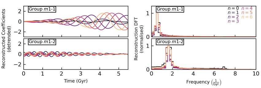
6     A. Johnson et al.
                                                                       that characterise the time evolution of a feature. Approx-
                                                                       imately equal values of dominant frequencies in the power
                                                                       spectra of the coefficient reconstructions between different
                                                                       PCs from mSSA of the same component suggest they are
                                                                       describing different aspects of the same feature and may be
                                                                       grouped together. If equal values occur across different com-
                                                                       ponents they may be mutually interacting. See the ‘DFT
                                                                       peak’ entry in Tables, which reports the frequency value
                                                                       where the DFT is maximised.
                                                                          We can also calculate contrast in the disc from the recon-
                                                                       structions6 . Calculating the average of the fractional devi-
                                                                       ation in surface density within one disc scalelength gives a
                                                                       measure of the ‘detectability’ of a feature (by eye or algo-
                                                                       rithm). See the ‘contrast’ entry in Tables. Related, the in-
                                                                       ferred location in the galaxy is where the dominant frequen-
                                                                       cies found in the power spectrum match the circular velocity
                                                                       of the unperturbed galaxy can indicate the spatial scales of
                                                                       any interactions taking place. Refer to Figure 1.
                                                                          In general, identified features evolve as one of the following
                                                                       types of evolution (noted in Tables): decaying, where a fea-
Figure 4. Disc monopole (m = 0) surface density as a function          ture peaks at the beginning of the simulation and decays in
of radius and time, computed from the full coefficient series (up-
                                                                       importance; growing, where the feature grows and then satu-
per panel), showing a largely featureless disc. The surface density
has been normalised by the central surface density. The remaining
                                                                       rates in amplitude with later maximum times therefore hav-
panels show the contribution to the surface density deviations for     ing slower growth rates; or consistent with no evolution. By
two groups of m = 0 principal components, identified as two dis-       comparing the evolution type across different components,
equilibrium signals (see Table 1). The surface density deviations      one may also infer causality. The relative growth or decay
are computed relative to the m = 0, n = 0 background, and are of       may indicate when one component is driving another.
the order a few per cent (excepting the outer disc, where the low
densities mean a variations naturally result in a larger per cent
variation).                                                            3.2 Initial Conditions Disequilibrium Uncovered
                                                                           Through Disc m = 0 Analysis

labelled ‘Group l1-1’. As PC groups capture trends in basis            We start our investigation with perhaps the most striking
function coefficients that are correlated over snapshots, PC           feature in the raw coefficients apparent in the top panel of
groups capture how spatial features dynamically evolve.                Figure 2 which shows the evolution of the m = 0 (monopole)
   Mathematically descriptive (but often difficult to interpret        disc coefficients. The figure suggests the simulation suffers
beyond the most significant few), the mSSA decomposition               from a disequilibrium that is typical in disc-halo initial con-
returns singular values (SVs) as measurements of the contri-           ditions: outwardly propagating rings in surface density. This
bution of each PC to the total decomposition. Larger SVs               section reports the insights into this apparent evolution af-
indicate which PCs represent more of the net change in time            forded by mSSA, starting from its application to the m = 0
of the distribution. This property greatly helps the robust            disc coefficients alone (3.2.1). The properties of the features
identification of features that represent true dynamical evo-          identified in this preliminary analysis provide a template for
lution. PCs which correspond to random fluctuations due to             further applications of mSSA both to the halo (separately
(e.g.) numerical noise are by nature uncorrelated. They have           and combined with the disc, see 3.2.2) and higher order disc
very low SV even as they may be the dominant source of                 terms (see 3.2.3). Table 1 summarises the properties of all
variations in the surface density. Conversely, PCs which de-           these analyses.
scribe evolution in coefficient series that are coherent over
time will have high SV even though they may be (orders of
                                                                       3.2.1 Grouping into Dynamical Features
magnitude) below the inherent noise. We report the singular
value fraction5 attributable to a given group in the Tables.           The mSSA analysis of the m = 0 disc reconstructed coeffi-
   We examine the coefficient reconstructions from a group of          cients reveals that PCs (0,1) and PCs (2,3,4,5) had distinct
PCs for physical insight. From the coefficient reconstructions,        power spectra, suggesting natural groupings. This also sug-
we can also construct power spectra from a Discrete Fourier            gested the presence of two distinct dynamical features with
Transform (DFTs) of the reconstructed coefficients from a              the signal in Figure 2. The properties of these two groups
group of PCs give insight into frequencies (and time scales)           that are quoted below are summarised in Table 1, with the
                                                                       rows labelled ‘Group m0-1’ and ‘Group m0-2’ corresponding
                                                                       to this first mSSA analysis.
5  To compute the relative contribution, we normalise each singular       Two more figures illustrate our results. Figure 4 shows the
value corresponding to a particular principal value to the sum of
all singular values. Then, we can say that some per cent of the
signal is represented by the principal component (or group). We        6 We do not look at the contrast in the halo, as this is not
will call this the contribution of a principal component (or group),   straightforwardly measured in real galaxies. Therefore, the con-
and may be interpreted as a measure of signal robustness.              trast columns do not contain entries for halo-only mSSA analyses.

MNRAS 000, 000–000 (2023)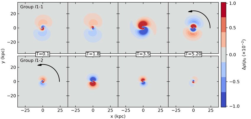
Near-equilibrium disc-halo dynamics                      7

Figure 5. An analysis of two groups obtained from the disc-only m = 1 mSSA decomposition. Each group corresponds to a distinct point
mode, discussed in the text as ‘Mode 1’ and ‘Mode 2’. The left panels show the reconstructed m = 1 coefficient amplitudes over time for
Groups m1-1 and m1-2. The right panels show the power spectra of the reconstructed m = 1 coefficients for each group. Both modes have
well-defined slow patterns – significantly slower than any frequency associated with stars in the disc – and show evolving behaviour: the
first mode is unstable and grows with time, while the second mode is damped and decays with time. The mode summaries are listed in
Table 2.

Figure 6. Normalised face-on (x, y) disc surface density deviation determined for two groups in the m = 1 decomposition. Each group
corresponds to a distinct point mode, discussed in the text as ‘Mode 1’ and ‘Mode 2’. The panels shows a reconstruction of snapshots
for either Group m1-1 (upper row) or Group m1-2 (lower row) in the disc-only m = 1 decomposition (cf. Figure 5). Both groups are
retrograde with respect to the disc rotation (rotation direction of the pattern is marked with an arrow). The mode shown in the upper
panels grows in amplitude over the course of the simulation; the mode shown in the lower panels decays in amplitude over the course of
the simulation, evident from the surface density features. Neither pattern strongly winds; both are a largely self-similar evolution, despite
being fairly tightly wound.

amplitude (left hand panel) and DFTs of the coefficient re-              relative to a smooth monopole background, constructed from
constructions for Groups m0-1 and m0-2, revealing their dis-             the two m = 0 PC groups.
tinct temporal characteristics. In Figure 3, we show the m = 0
surface density amplitude reconstruction as a function of disc              Overall, we find the following characteristics.
radius (y-axis) and time (x-axis) from the unprocessed coef-             Group m0-1 represents a dynamical feature that shows weak
ficients (top panel), as well as the surface density deviations          evolution over the entire simulations with a surface den-
                                                                         sity contrast of approximately 3 per cent. The slow decay
                                                                         of Group m0-1 produces power at a range of very low fre-

                                                                                                              MNRAS 000, 000–000 (2023)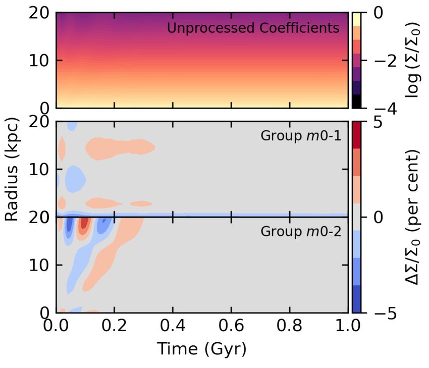
8     A. Johnson et al.

                                                                       Figure 8. Description of the strongest principal component group
                                                                       for halo and disc decompositions: a growing multi-component point
                                                                       mode. The upper panel shows the detrended and normalised am-
                                                                       plitude of the reconstructed cosine component of the m = 1 (disc;
                                                                       grey curves) or l = 1 (halo; black curves) n = 0 coefficient ver-
                                                                       sus time. The solid curves are for mSSA decompositions run on
                                                                       each component alone (Group m1-1 and Group l1-1). The dashed
Figure 7. Amplitude and phase as a function of radius and time         curves are for the joint halo+disc mSSA decomposition (Group
for the disc-only m = 1 decomposition for the first two groups iden-   m1l1-1). The lower panel shows the power spectrum (DFT ampli-
tified in the mSSA analysis. Each group corresponds to a distinct      tude vs frequency), for the four series shown in the upper panel.
point mode. From top to bottom, we show the amplitude and phase        The relative similarity of the curves and power spectra suggests
for the unprocessed m = 1 coefficient streams, the reconstructed       that the patterns are correlated between the disc and halo. The
coefficients of Group m1-1, and the reconstructed coefficients of      slow growth of the disc amplitude over time relative to the larger
Group m1-2. The density is shown as the log of the absolute value      halo amplitude at the outset of the simulation suggests that the
of the density. Both groups show coherent phases identifiable in       halo is responsible for driving the mode.
the seemingly random phase information of the unprocessed co-
efficients. The growing (decaying) nature of Group m1-1 (Group
m1-2) is also evident in the amplitudes.                               quencies, peaked at 0.2Gyr−1 .
                                                                       Group m0-2 shows outwardly propagating rings in surface
                                                                       density that start at the beginning of the simulation and dis-
                                                                       appear after ≈ 1 Gyr, losing speed as they move to larger
                                                                       radii. While this is a sub-1 per cent effect within a disc scale
                                                                       length, at larger radii, the surface density deviation is obvi-
                                                                       ous by eye as ringing features. The periodic nature of Group
                                                                       m0-2 corresponds to a frequency peak at 6.4Gyr−1 .
                                                                         We conclude that mSSA has cleanly separated two distinct
                                                                       evolutionary processes operating simultaneously within one
                                                                       harmonic term. The next two subsections explore the nature
                                                                       of both of these features.

                                                                       3.2.2 Group 1: Halo-driven disequilibrium?
                                                                       The appearance of Group m0-1, at low frequency, suggests
                                                                       that its origin may be connected to the halo, where timescales
                                                                       are naturally long. Specifically, the frequency 0.2 Gyr−1 cor-
                                                                       responds to a circular orbit at R ∼ 50 kpc (see Figure
                                                                       1). This motivated us to apply mSSA to the l = 0 coeffi-
                                                                       cients representing the halo component in the simulation to
                                                                       explore this connection further. We run analyses of both the
                                                                       halo l = 0 alone and in combination with the disc m = 0
                                                                       coefficients.
                                                                          The results of the analysis of the halo alone is shown in
                                                                       lower panels of Figure 3 and summarised in the second row
                                                                       of Table 1. These demonstrate that the readjustment of the
                                                                       halo component’s radial profile is even more significant than

MNRAS 000, 000–000 (2023)
Near-equilibrium disc-halo dynamics 9
Figure 9. Normalised face-on (x, y) halo z = 0 plane density deviation reconstruction snapshots for Group m1l1-1 (upper panels) and
Group m1l1-2 (lower panels) in the halo-and-disc l = 1 + m = 1 decomposition. Each group corresponds to a distinct point mode.
The patterns extends to large radii in the halo and are retrograde with respect to the disc rotation. The halo reconstructions exhibit
significantly less ordered behaviour compared to the disc owing to the three-dimensional nature of the mode, which also tips relative to
the z = 0 plane. However, the bulk properties are similar to the disc (cf. Figure 6). The mode summaries are listed in Table 2. That the
joint decomposition of the halo and disc returns the same groups, with similar behaviour, is strong evidence for the mutual mode nature
of the features. The large spatial scale of the modes in the halo, coupled with their relatively early coherence, is suggestive that the modes
are induced by the halo.
the disc radial profile, with a signal amplitude twice as strong Even disc harmonics (m = 2, 4, 6) show a persistent signal in
as the disc (compare detrended amplitudes in Figure 3). Such the most important PCs (0 and 1) with a pattern speed of
halo-driven disequilibrium is also a common feature for nu- ∼ 3.3 cycles/Gyr that is equal to the half the Group m0-2
merical realisations of multi-component galaxies as their com- frequency peak of 6.6 cycles/Gyr7 . Note that the joint analy-
bined equilibrium properties have been approximated, for ex- sis of all even disc harmonics (m = 2, 4, 6) returns essentially
ample through Jeans modelling or adiabatic contraction cor- the same results as the m = 2 only decomposition. In the
rections. Thus the mass distribution of the halo adjusts to case of harmonic orders m > 2, this result likely owes to the
full equilibrium in the presence of the disc, and vice versa. need for higher order harmonics to fully represent the feature
In Table 1, a comparison of rows 1 (analysis disc coeffi- being described.
cients alone), 2 (halo coefficients alone) and 3 (disc and halo The remaining rows of Table 1 demonstrate that the Group
coefficients combined) confirms: (i) all three mSSA analyses m0-2 disc disequilibrium signal is also evident at a lower
have similar temporal structures, corresponding to the dy- level (i.e. higher PC numbers, lower contrast in the disc and
namical timescales at several tens of kpc in the system; (ii) smaller SV) in both the disc m = 1 and halo l = 1 decom-
the joint disc/halo analysis actually identifies the same co- positions when comparing frequency structure of the groups.
herent features in the disc and at greater contrast (0.054 vs While the peak surface density deviation is near the outset of
0.031) than the disc analysis alone; (iii) that the driver for the the simulation for m = 0, in higher harmonic orders the sig-
combined evolution is likely the halo given the larger ampli- nal does not completely fade over the simulation, with peak
tude of its coherent changes relative to random fluctuations measured contrasts coming at later times. Our findings show
for that component. the utility of mSSA in detecting evolution incited across dif-
The above results demonstrate the ability of mSSA to suc- ferent harmonic orders.
cessfully identified the mutual readjustment of the coupled
disc-halo system from a mild disequilibrium state.
3.2.3 Group 2: Disc-driven disequilibrium
The strength of Group m0-2 in the analysis inspired an in-
vestigation as to whether this disequilibrium could also seed 7 The pattern speed of a harmonic is the number of cycles per
other features in the simulation. Examination of other mSSA Gyr divided by the harmonic number. That is, the pattern speed
decompositions for different coefficient combinations finds of the disc-only decomposition of Group 2 m harmonic coefficients
many similar-frequency signals (see lower rows of Table 1). is Ωm = ΩDFT /m cycles/Gyr.
MNRAS 000, 000–000 (2023)10 A. Johnson et al.
3.2.4 Key insights frequency of the signal (Ω = 0.6 cycles/Gyr) is located near
the scale radius of the halo, well outside the disc8 . Mode 1
In this section, BFE+mSSA has been used to increase our
grows significantly in amplitude over the simulation, with the
understanding of a dynamical simulation by:
peak surface density signal coming near the end of the simu-
(i) separating distinct evolutionary pathways within a single
lation. Computing the contrast in the outer, low-density disc
harmonic;
(r > 12 kpc), the surface density deviation amplitude reaches
(ii) identifying coupling between multiple components;
10 per cent, detectable as lopsidedness in deep imaging of disc
(iii) detecting features across different harmonics within a
galaxies.
single component.
Mode 2 groups m = 1 PCs 2 and 3, reconstructing a
These results emphasise that initial conditions for near
slowly rotating, slowly decaying mode. The frequency of the
equilibrium studies of galaxy evolution need to be dynam-
signal (Ω = 1.7 cycles/Gyr) is located closer to the Galactic
ically relaxed (or virialised) by evolving in isolation for tens
centre, but also beyond the bulk of the disc mass. Mode 2
of halo dynamical times (i.e. much longer than than the
decays from the outset of the simulation, and is significantly
equivalent timescale in the disc) prior to an studies of in-
weaker than the first mode, with a peak contrast of order 0.1
teractions in order to truly isolate signatures of the external
per cent within a scale length.
perturbation. While the perturbation in our study is a nu-
merical artifact, the distinct adjustments to density profiles
and couplings within and across components uncovered by 3.3.2 Connection between the disc and halo
BFE+mSSA represent the drivers of the evolution of galax-
ies seeded by any perturbation. Since the frequencies of the two modes are consistent with
halo frequencies we naturally suspect that the halo is sup-
porting the modes. To test this, we perform additional mSSA
3.3 Secular evolution signals Uncovered Through decompositions: first with the l = 1 halo coefficients alone,
Disc m = 1 Analysis and then with the l = 1 halo coefficients jointly with the
m = 1 disc coefficients9 . The results of the runs are sum-
Examination of the PCs from the mSSA decomposition of the
marised in Table 2. We find sets of PCs in the halo-only
dipole disc harmonic (m = 1) revealed two groups, with prop-
decompositions corresponding to Modes 1 and 2, which we
erties summarised in Table 2 and contributing coefficients
associate by means of their similar frequencies. We also find
and power spectra visualised in the left and right panels of
corresponding PCs in the joint disc-halo decomposition. The
Figure 5. Examination of the power spectra show that these
joint analysis in particular suggests that the modes are multi-
features are distinct in nature to the disequilibrium-seeded
component in nature, owing to the similar properties between
m = 0-dominated Groups m0-1 and m0-2 described in the
all decompositions.
previous section in that they have clear, well-defined frequen-
Figure 8 provides an example visualisation for a single ra-
cies, rather than a broad spectrum. This indicates that each
dial coefficient (n = 0) contributing to Mode 1 to verify
of these groups may be a point mode present in the system. As
this interpretation. Comparing the coefficients reconstructed
discussed in Section 2.1, point modes are a result of the fun-
from identified in the independent analyses of the disc and
damental properties of the underlying phase-space distribu-
halo (solid lines), as well as the joint disc-halo decomposition
tion. They have single-valued real and imaginary frequencies
(dashed lines), we find the same features are identified in both
(hence the descriptive point) that describe the periodicity and
the combined and independent analyses: the curves in the
growth or decay of the features they support. These modes
upper panel of Figure 8 are unchanged whether the decom-
drive secular, self-sustained evolution distinct from that of
position is performed on a per-component basis, or jointly.
a transient response to an external driver (e.g. the disequi-
This implies that the same principal component can describe
librium initial conditions in the previous section) that phase
the evolution in both the disc and halo, and that the sig-
mixes away. Hence we refer to these groups as ‘Mode 1’ and
nal is strong enough in both components to be identified in
‘Mode 2’, and examine their nature in the following subsec-
per-component analyses. This is a strong indication of a cor-
tions. In the disc m = 1 analysis, these are Groups m1-1 and
related multi-component signal. In general the same features
m1-2.
will not be recovered from combined analysis of different com-
ponents because the inter-component decomposition need not
3.3.1 Appearance of modes in the disc match the intra-component decomposition. In contrast, our
joint analysis finds a single PC group may be used to recon-
We augment the information about the two modes sum- struct the modes in both the disc and the halo, identifying
marised in Figure 5 and Table 2 with visualisations of their them as a mutual mode.
appearance in Figures 6 and 7. Figure 6 shows selected face-
on disc surface density reconstructions to demonstrate that
8 For m > 0 harmonics, PC groupings frequently occur in pairs
both modes create spiral patterns that are retrograde relative
to the rotation of the disc. Figure 7 illustrates the radial (y- that describe both the amplitude and phase of a feature. In the left
axis) and time (x-axis) evolution of the surface density (upper hand panels of Figure 5 only the cosine terms in the coefficients are
plotted to allow the reader to infer both amplitude and periodicity.
panel in each pair) and phase over (lower panel in each pair) 9 To find correlated features between the halo and disc we choose
for the full time sequence, indicating both the growth/decay halo coefficients that can describe features with meaningful projec-
and periodicity. Inspection of these figures and the table pro- tions into the disc plane. To this end we choose only the Ylm = Y11
vide the full characterisation of the modes. terms of the halo expansion, excluding the Y10 term. In addition
Mode 1 groups m = 1 PCs 0 and 1, reconstructing a we use the same number of coefficients from each component to
slowly rotating, growing mode. Referring to Figure 1, the avoid introducing the prior of unequal representation.
MNRAS 000, 000–000 (2023)Near-equilibrium disc-halo dynamics 11
For both modes, we can examine and compare timescales 3.4 Fluctuations and other uninterpretable features
and amplitudes to try to understand the driver of the evolu-
In the two previous sections, we identified interpretable sig-
tion. Comparing between components, the feature strength
nals in various harmonics of both the disc and halo coeffi-
is higher in the halo at earlier times in each mode (of order
cients in groups of low-order PCs using BFE+mSSA. How-
1% density contrast in the halo, but well below that in the
ever, inspection of the last column of Tables 1 and 2 shows
disc), implying that the halo is responsible for starting each
that these PC groups only contain a fraction of the total sin-
mode at large radii (compare Figures 6 and 9). For the grow-
gular values (which are normalised to total unity): most of
ing Mode 1, estimating the growth rate from the modulus of
the groups represent less than 20 per cent of the variance
the coefficients at early times also reveals the growth of the
in the coefficients being analysed10 . The rest of the signal
halo feature to be twice that of the disc. The saturation point
spread over many (many!) higher-order PCs with lower SVs.
of the halo is also measurably earlier than the disc (T = 2.2
These are PCs with very weak self-gravity. We refer to these
Gyr in the halo vs T = 3.2 Gyr in the halo).
remaining terms as the nullity, owing to its uninterpretable
The comparison of the disc and halo features in the pre-
nature: it will contain numerical noise, but may also contain
vious paragraph suggest that the modes may arise from
signals too weak to be included in our analysis.
a fundamental dynamical property of the halo component.
To understand the properties of the nullity, we collect all
Figure 9 shows snapshots of the halo feature during the
uninterpretable PCs for a given mSSA decomposition and
simulation at times corresponding to Figure 6. The fea-
analyse their reconstructions, summarising the results for
tures are both slow retrograde pattern which build and/or
low-order disc harmonics in Figure 10 and for all decompo-
damp over time. They bear hallmarks – a slow dipole pat-
sitions in Table 3. Figure 10 shows the reconstructed coef-
tern at relatively large scales – of the weakly damped l =
ficients and corresponding power spectrum for the PCs as-
1 modes in spherical systems that have been studied in
signed to the nullity for low-order disc harmonics. Compar-
using linear perturbation theory. These were first identi-
ing this to the corresponding Figures 4 and 5 for lower or-
fied by Weinberg (1994), and later additionally reported by
der PCs, the difference is clear. The bottom panels for the
Heggie et al. (2020), Fouvry & Prunet (2021), and Weinberg
m = 2 nullity do have hints of a signal in the form of low-
(2022).
level systematic evolution in the left hand panel and some
We conclude that BFE+mSSA has allowed us to detect and
clear peaks in the right panel. We discuss future strategies
characterise slow, secular evolution of our isolated simulated
to hunt for weak signals in Section 4.1. However, in general,
galaxy due to the nature of the underlying equilibrium.
there is a lack of periodic or systematic evolution in the left
hand panels and flat spectra of frequencies in the right hand
3.3.3 Key insights panel, characteristic of noise. A comparison of the contrast
columns of Tables 3, A1 and 2 shows that the fluctuations
The results in this section provide additional illustrations of in the surface density derived from the nullity are mostly
the ability of BFE+mSSA to separate evolutionary pathways stronger than the coherent signals in this particular simula-
in a single harmonic and to detect coupling across compo- tion: our BFE+mSSA analysis has supported insights that
nents. would otherwise be inaccessible.
Most significantly, BFE+mSSA allowed the detection of
slow, low-level secular evolution in our simulation that
had been predicted in analytic work, (Weinberg 1994;
Fouvry & Prunet 2021) and recently observed in star cluster 4 LOOKING AHEAD
and dark-matter-halo-only simulations (Heggie et al. 2020; 4.1 Essential Future Work - assessment of weak
Weinberg 2022). The analytic work suggests that spherical feature significance
systems, such as dark matter halos, generically exhibit dipole
point modes. The common existence of these modes has im- Our analyses of simulations of bar formation
portant implications for understanding lopsidedness in galax- (Weinberg & Petersen 2021; Petersen et al. 2022) and
ies: the halo and disc mutually open dynamical avenues that an isolated disc galaxy (this paper) amply illustrate the
cannot be taken by either component independently; there- facility of BFE+mSSA to learn about both significant and
fore many dynamical features are simply inexplicable without expected as well as subtle and unanticipated dynamical evo-
an understanding of the interplay between components. How- lution. The results are very promising for general applications
ever, making a clear connection between the theory and ob- to a wide variety of dynamical systems. However, our work
served galaxies has been hampered by the technical challenge so far has been involved close supervision of BFE+mSSA
of applying analytic work to multi-component systems. More- to both interpret and understand the significance of what
over, while numerical simulations routinely represent multiple features it has identified.
component systems, the description of the results is typically In particular, the interpretative ambiguity we encountered
limited to visualisations and statistical analyses that can only in the higher order terms in this paper outlines the current
qualitatively be connected to dynamical drivers. limit of BFE+mSSA. This limit motivates the need for a rig-
BFE+mSSA has bridged this gap by clearly showing an orous statistical analysis of significance for mSSA-identified
l = 1 mode in our simulated halo driving lopsidedness in signals. Many of the well-known approaches from statistical
our simulated disc. These results speak to the promise of
BFE+mSSA for forging the missing connection between the- 10 The exception are some of the PCs associated with the
ory, simulations, and observations needed to interpret galac- monopole, which encode the equilibrium. These PCs are respon-
tic properties in terms of our fundamental dynamical under- sible for upwards of 60 per cent of the singular value signal, cf.
standing secular evolution. Table 1.
MNRAS 000, 000–000 (2023)12 A. Johnson et al.
Figure 10. An analysis of the content in the nullity for m = 0 (upper panels), m = 1 (middle panels), and m = 2) lower panels. The
left panels show the reconstructed nullity coefficient amplitudes over time for m = 0, 1, 2 (top to bottom). The right panels show power
spectrum of the reconstructed nullity coefficients for each harmonic. Both m = 0 and m = 1 show no discernible signals. The m = 2
harmonic shows some periodicity, but the power spectrum suggests the frequencies are broad and not strongly coherent. Therefore, we
are confident that we are not throwing away interpretable signal in the nullity in any harmonics. These reconstructions may be compare
to the unprocessed coefficients, Figure 2, for a quantitative analysis of what signals are part of coherent signal groups.
mSSA PCs DFT peak contrast SV
decomposition (Gyr−1 ) (R < Rd ) fraction
disc m = 0 6+ - 0.005 0.275
disc m = 1 6+ - 0.008 0.678
disc m = 2 2+ - 0.017 0.799
disc m = 3 2+ - 0.012 0.936
disc m = 4 2+ - 0.010 0.914
disc m = 5 2+ - 0.006 0.954
disc m = 6 2+ - 0.005 0.964
disc m = 1, 3, 5 2+ - 0.027 0.933
disc m = 2, 4, 6 2+ - 0.037 0.928
halo l = 0 6+ - - 0.028
halo l = 1 6+ - - 0.693
disc m = 0, halo l = 0 6+ - 0.021 0.130
disc m = 1, halo l = 1 8+ - 0.010 0.667
disc m = 1, 2, halo l = 1 4+ - 0.012 0.801
Table 3. Summary of principal components assigned the nullity in our decompositions. We refer to each collection of PCs here as the
‘Nullity’, rather than a PC group. Disc harmonics are denoted with m, halo harmonics are denoted with l. Columns are the same as in
Table 1.
analysis would be suitable for this purpose. For example, let corresponding to the signal in question is beyond the pre-
us take the hypothesis that the signal observed at m = 2, 3, 4 diction intervals, the corresponding principal component is
is consistent with background noise as a test case. That is, our considered significant. In such a case, the signal can be re-
null hypothesis is that our simulation can generate with the liably reconstructed. This approach is often called Markov
same properties of the signal in question without inherent self Chain SSA (MC-SSA, see Allen & Smith 1996).
gravity. To do this, we need to generate a simulation with the
same noise spectrum as the full simulation but without any Analyses of this sort are particularly well-suited to the exp
self-gravitating features on the spatial and temporal scales of framework described in Petersen et al. (2022). We can use the
our putative signal. Let us assume that we know how to per- mSSA analysis to construct a realistic reconstruction of the
form such simulations (we propose an exp-enabled approach coefficients series from the self-gravitating simulation with-
below). An ensemble of these null-hypothesis simulations can out the self-gravitating features of interest by removing the
be run and analysed using mSSA. From the ensemble of sim- groups corresponding to the signal in question. In the study
ulations, one may construct prediction intervals for singular presented here, this would be akin to retaining only the nul-
values under the null hypothesis. Then, if the singular value lity reconstructions of the coefficients. We can generate new
MNRAS 000, 000–000 (2023)Near-equilibrium disc-halo dynamics 13
coefficient series from an autoregressive model11 consistent Understanding of noise. There have been many years of de-
with the coefficient covariance from the mSSA reconstruc- bate on the effect of noise in conclusions drawn from dynami-
tion. Then, exp allows initial potential fields from the re- cal simulations, from bar-halo interactions (Weinberg & Katz
constructed coefficients to be replayed for a new ensemble 2007), through dynamical friction (Weinberg 2001), to satel-
of particles with very little computational effort. The result- lite disruption (Errani & Peñarrubia 2020). BFE+mSSA
ing expansion coefficient series are gathered automatically clearly separates the correlated, quasi-periodic signals result-
for analysis by mSSA, and can be analysed for significance ing from dynamical interaction and coupling from the fluctu-
of detected features. A detailed description of the MC-SSA ating forces resulting from finite particle number stochastic
approach in the exp context will be described in a later con- effects. We expect that couplings in orbital dynamics have
tribution. frequencies near or smaller than the characteristic orbital
frequencies. Since the individual PCs describe the tempo-
ral behaviour of components assigned to the noise field and
4.2 Prospects for applications to simulations the power spectrum describes their characteristic frequencies,
Despite the limitations, there are multitude of prospects for mSSA provides a natural classification of signal and noise.
immediate, supervised applications of BFE+mSSA to simu- Investigations of test-particle orbits with and without the
lations of galaxies, whether isolated, interacting or evolving noise component provide a diagnostic tool for the reliability
in the full cosmological context. of features in simulations and the role of fluctuations more
generally.
Dynamical analyses of simulations of galactic evolution.
Recent surveys (Majewski et al. 2017; Steinmetz et al.
2020; Gaia Collaboration et al. 2022) demonstrate that the
Milky Way continues to evolve through satellite interaction. 5 CONCLUSIONS
N -body simulations have explained some key observational
signatures (Laporte et al. 2019; Petersen & Peñarrubia 5.1 Near-equilibrium evolution: the importance of
2020; Garavito-Camargo et al. 2021a; Vasiliev et al. 2021; multi-component modes
Hunt et al. 2022a). However, interpretation of these We applied BFE+mSSA to a simulation of an isolated Milky
simulations is challenging since many actors contribute Way like galaxy. The BFE+mSSA combination allows us
simultaneously. The BFE+mSSA knowledge discovery ap- to automatically identify the main features in the model
proach is capable of separating, characterising and dissecting galaxy and their origins. Most remarkably, BFE+mSSA
the signatures of the mutual interactions of each component achieved this in the challenging case of an isolated, multi-
in simulations by separating features by correlating tem- component galaxy that had specifically been constructed to
poral and spatial scales non-parametrically. BFE+mSSA not evolve and where the dynamical signatures were below
promise detailed predictions and identification of features the level of the noise. Our work complements a prior investi-
in current stellar data sets (see Petersen & Peñarrubia gation (Weinberg & Petersen 2021) which used BFE+mSSA
2021; Garavito-Camargo et al. 2021b; Lilleengen et al. 2022, to characterise significant evolution of known nature in a sim-
for some recent results) and confident mapping the the ulation which formed a galactic bar.
dark matter halo’s global structure and distortions to that In our near-equilibrium model, we identified – for the
structure. This goal was unimaginable even 5 years ago. first time – two multi-component (disc-halo) dipole point
Structural characterisation and correlation of fields. This modes (Figures 5-8) which evolve over time (one growing,
paper demonstrated the discovery of two-dimensional fea- one damped; Table 2). This discovery is enabled by the
tures in disc density resulting from internal (disequilibrium- BFE+mSSA methodology; such dynamical effects are at a
related) dynamics and halo interactions. However, level such that other methods, such as Fourier analyses,
BFE+mSSA can be applied to any field in any num- will not be able to recover the signals. Halo modes are
ber of dimensions. For example, Weinberg & Petersen expected from linear perturbation theory (Weinberg 1994;
(2021) illustrated a three-dimensional disc BFE. The exp Fouvry & Prunet 2021), and are observed in simulations
library already enables joint BFE+mSSA investigations of star clusters (Heggie et al. 2020) and dark matter halos
of any number of three-dimensional density and potential (Weinberg 2022), but the coupling of a spheroid to a disc
fields. These may be augmented by kinematic fields as in has not been discovered to date. The BFE+mSSA methodol-
Weinberg & Petersen (2021) or some other field such as ogy makes the identification of point modes straightforward,
star formation rates and implied local metallicity. If the and provides several avenues for corroboration. We employed
additional fields encode spatial information (e.g. they are several different mSSA decompositions to validate our find-
BFE coefficients or even radial and azimuthal bins), their ings. The existence of point modes in these isolated simula-
temporal and spatial scales will be correlated with the tions demonstrates the fundamental contribution of compo-
density and potential fields. The BFE+mSSA can adapt to nent interactions to the dynamical evolution of galaxies. We
new observational tools and windows as new surveys become expect that the existence of such multi-component disc-halo
available. modes is a generic feature of such systems, possibly including
the Milky Way. These modes likely have influence over the
11 Autoregressive noise models are typically used for null hypothe- structural evolution of disc galaxies. For instance, our results
ses in MC-SSA because SSA provides good estimates for frequen- immediately suggest that low dipole modes will be most de-
cies and exponential factors processes generated by the related lin- tectable at large radii (e.g. R > 20 kpc in the Milky Way),
ear recurrence relations (Golyandina & Zhigljavsky 2013, Section where density contrasts can exceed 10 per cent relative to a
3). smooth disc.
MNRAS 000, 000–000 (2023)You can also read